PROGRESS TOWARDS A METHOD FOR PREDICTING AUV DERIVATIVES
E.A. de Barros 1, A. Pascoal 2, E. de Sa 3
1- Department of Mechatronics Engineering and Mechanical Systems, University of São Paulo. SP. Brazil. Email:
[email protected] 2- Institute for Systems and Robotics (ISR), Dept. of Electrical Engineering and Computers, Instituto Superior Técnico Lisbon. Portugal. Email:
[email protected] 3- National Institute of Oceanography. Dona Paula. Goa. India. Email:
[email protected]
Abstract: The paper addresses the problem of autonomous underwater vehicle (AUV) modeling and parameter estimation as a means to predict the expected dynamic performance of underwater vehicles and thus provide solid guidelines during the design phase. The use of analytical and semi-empirical (ASE) methods to predict the hydrodynamic derivatives of the most popular class of AUVs is discussed. An application is made to the estimation of hydrodynamic derivatives of the MAYA AUV, an autonomous underwater vehicle that is being developed under a joint IndianPortuguese project. The estimates were used to predict the turning diameter during a sea trial. Keywords: AUV, Hydrodynamic Derivatives, Prediction Method, Manoeuvring, Slender Body.
1. INTRODUCTION The prediction of AUV maneuvering performance is important during the preliminary design phase. Techniques for estimating aerodynamic coefficients of vehicles have been developed originally for airships, and later refined for aircrafts, missiles, and submarines. Methods for estimating hydrodynamic derivatives have also been used in the ship industry for decades. Recently, spawned by the widespread availability of powerful computers there has also been a surge of interest in applying Computational Fluid Dynamics (CFD) for constructing the flow field and calculating the pressure distribution acting upon a submerged marine vehicle. From such maps, the resulting forces and moments of interest acting on the vehicle can then be calculated. However, to investigate the maneuver performance of these vehicles, it is still customary to represent fluid forces and moments in terms of coefficients expressing the sensitivity of
each force and moment to each component of the velocity and acceleration of the vehicle itself, as well as to the control surface deflections. After determining the coefficients, motion simulators are implemented, where maneuver performance and control techniques can be easily evaluated. Therefore, most of the prediction methods are directly focused on the estimation of parameters such as added mass and inertias (acceleration related coefficients), linear and non-linear damping coefficients (related to velocities) and control action related parameters. Tank tests using a constrained vehicle model can be employed for estimating hydrodynamic coefficients. Another experimental approach is based on free running models, tested in basins or in natural areas (lakes, open sea, etc.). Both approaches are time consuming and expensive. They involve model building, testing, analyzing, and interpreting the results. Costs can be even higher, if the option to rely on an experimental approach is taken at the preliminary design phase. In fact, the vehicle
configuration may be changed many times, for nonhydrodynamic related reasons, thus reducing considerably the usefulness of early test results. Analytical and semi-empirical methods (ASE) for predicting hydrodynamic derivatives provide approximate results that can be applied for predicting maneuverability characteristics, selecting hydroplanes, and investigating control strategies at an early stage, in a new design. Advanced approaches to AUV design may also involve combined plant/controller optimization, where prediction methods of hydrodynamic derivatives play an important role (Silvestre et al., 1998). This paper addresses the development of analytical and semi-empirical methods for prediction of AUV maneuverability characteristics. This work reports the progress achieved in the effort of developing formulations for predicting the hydrodynamic derivatives of submerged bodies and is the natural continuation of the study presented by the authors in a former paper (de Barros et al., 2004). An application is made to the estimation of a set of derivatives for the MAYA AUV, an autonomous vehicle that is being developed under a joint Indian-Portuguese project. The paper is organized as follows. Section 2 introduces the main concepts and formulas that have been investigated for defining the ASE method for computing the full set of hydrodynamic derivatives for the MAYA derivatives. Section 3 presents the stability derivatives as a combination of the parameters described in section 2. Section 4 describes the experiments on maneuvers using the MAYA AUV for comparing results predicted by the ASE methods and those from the tests. Finally, section 5 provides a critical review of results obtained and indicates future steps in the research. 2. ANALYTICAL AND SEMI-EMPIRICAL FORMULATIONS Analytical and semi-empirical methods for the estimation of the hydrodynamic derivatives of marine vehicles are well rooted in the theory of hydrodynamics. The use of a particular method is decided by taking into consideration the physical nature of each of the parameters to be estimated, together with the underlying simplified assumptions adopted when modeling the vehicle. In what follows, the computation of hydrodynamic coefficients of a fully submerged vehicle is organized in groups according to the type of effort considered, and divided into the relevant geometrical parts that compose the vehicle (bare hull, fins, and annular foil or duct) and their combination. In what follows, the vehicle length L and its powers are used for adapting the formulas to the non-dimensional standards of SNAME (SNAME, 1950). Forces and moments considered are referred to the body axis system (Fig. 1) whose origin is at the vehicle centre of mass.
Fig. 1. Representation of the Vehicle Body-Axis System and lift surface angles.
2.1 Bare Hull Coefficients The hull axisymmetric geometry was studied, and particularly the shape proposed by Myring (1976) was chosen for calculations and experimental validation. This kind of hull shape provides practical advantages for the designer, related to the availability of inner space for carrying equipments, while keeping the more streamlined characteristics outside when compared to torpedo shapes. It is a common shape for AUVs (such as REMUS and MAYA); this makes the predicted coefficients part of a significant data base, which can serve as a basis for AUV design. The bare hull parameters used in the Myring shape that was considered are included in table 1. Table 1 Main parameters of the Hull Bare Hull Length(m)
1.742
Hull Maximum Diameter (m) Base Diameter (m) Nose Length (m) Middle Body Length (m) Myring Body Parameter θ (o) Myring Body Parameter n
0.234 0.057 0.217 1.246 25 2
In the work of Myring (1976), the drag was estimated using the calculation of the axisymmetric boundary layer. Less laborious methods can provide similar results (Chappell, 1978). They are based on the knowledge of the fineness ratio of the body (rate of the body length to its maximum diameter). The adapted formula of Datcom belongs to the later approach, and was adopted in this work (see Hoak, D.,and Finck ,1978): S CD* = C f ⎡⎣1 + 60 f −3 + 0.0025 f ⎤⎦ S2 L
where Ss is the body wetted area, and
(1)
Cf =
0.075
( log Re− 2 )
2
+ 0.00025
x* = 0.378 ⋅ L + 0.527 ⋅ x1
(2)
is the estimate of the skin friction drag coefficient, according to ITTC. The parameter f is the fineness ratio of the body, f = L d , relating the body length to its maximum diameter. This result should be added to the base-drag coefficient, which is given by:
The same approach was used for adapting the slender body theory result to the computation of the lift moment coefficient, using also the volume V*, between the nose tip and the station at x*. Manipulating the Datcom formula gives: (Cmα ) B =
3
CD
b
S ⎛d ⎞ = 0.029 ⎜ b ⎟ (CD* ) −0.5 N2 L ⎝d ⎠
(3)
where SN is the cross sectional area at the end of the nose section
x0 (CLα ) B V * − S * x* + 2(k2 − k1 ) L L3
⎛ L − x0 ⎞ (CLq ) B = (CLα ) B ⋅ ⎜ ⎟ ⎝ L ⎠
(4)
The moment coefficient is approximated by:
The lift coefficient, when calculated by slender-body theory for a body of revolution, is equal to 2, based on the base area. For a vehicle with a “Myring shape”, composed of forebody, cylinder, and afterbody, applying such an approach blindly means that one neglects the vortex and separation produced by viscous effects at the tail region. In a number of AUVs, such as MAYA, the presence of appendages may even intensify the break down of the ideal flow hypothesis before this region of the body. On the other hand, considering the slender-body method only up to the end of the nose section (de Barros et al., 2004), as in the case of missiles with a blunt base, means to neglect the pressure distribution at the tail. In this case, applying the Datcom expression for calculating the lift coefficient yields:
⎛ L − x0 ⎞ ( xC − x0 ) (Cmq ) B = −(CLα ) B ⋅ ⎜ ⋅V ⎟ + L4 ⎝ L ⎠
⎛ ∂CLα ⎞ 2 ⋅ (k2 − k1 ) ⋅ S N (CLα ) B = ⎜ ⎟ = L2 ⎝ ∂α ⎠α = 0
+ 0.73
2 ⋅ (k2 − k1 ) ⋅ S * L2
2
(11)
where, xC is the body centroid distance from the nose tip and V is the body volume. The computation of added mass coefficients is based on ideal fluid flow theory. A number of reliable numerical methods are available for the estimation of this kind of parameters. Source distribution and panel methods are the most common numerical techniques. Approximating the hull as an ellipsoid, and obtaining the parameters from analytical calculations is a simplified approach. This last option was chosen by the authors for calculating the surge added mass. For the other coefficients, the strip method was applied (Newman, 1977). 2.2 Lift and Drag Produced by Small Aspect Ratio Fins
(6)
The intermediate solution chosen was to use the Datcom method to estimate the position of the body, x0, where the ideal flow hypothesis is no longer valid, and use the cross sectional area at such station, S*, as the reference area for the lift coefficient:
( CLα )B =
(10)
(5)
where “k2-k1” is the “Munk” apparent mass factor. For the fineness ratio interval between 4 and 19, this factor can be calculated by:
( k2 − k1 ) = −0.0006548 f 2 + 0.0256 f
(9)
The body dynamic coefficients were also calculated based on slender body theory. The lift coefficient is given by:
The total body drag coefficient is then calculated: CD0 = CD* + CDb
(8)
(7)
The estimative of the position x* is based on the station x1, where the body profile has the most negative slope in the aft direction. The semi-empirical relation is given by (Hoak and Fink, 1978):
The most extensive study on this matter, related to marine applications, was developed by Wicker and Fehlner (1958), who proposed semi-empirical expressions adopted by authors in ship and submarine maneuvering models (Lewis, 1989, Bohlmann, 1990). The lift coefficient is calculated from: CLαW AR
=
2π ⎞ 1 ⎛ AR 2 + 4 cos 2 Λ c / 4 ⎟ 2+ 2 ⎜ 2 n ⎝ cos Λ c / 4 ⎠
(12)
where, AR is the lift surface aspect ratio, Λc/4 is the sweep angle at one fourth of the chord length, and ηis a factor to correct for viscous effects. Foil drag contributions were also included into the derivatives. Based on the semi-empirical expression proposed by Hoerner (1965) for streamlined shapes at
low Reynolds numbers, the foil drag coefficient is calculated by: −1
t t S ( CD 0 )F = [2 ⋅ C f ⋅ ⎛⎜ ⎞⎟ + 2 ⋅ C f + ] f (2F ) c L ⎝c⎠
(13)
where, “t” is the foil maximum thickness, “c”, the corresponding chord, and Sf(F) is the maximum cross sectional area. 2.3 Fins and Body Combination 2.3.1 Vertical Plane Theoretical and semi-empirical approaches have been proposed from the marine field (Lewis, 1988), and aircraft dynamics (Hoak and Finck, 1978; Gilbey, 1993) for modeling the lift produced by a vertical fin in the presence of a body of revolution. Basically, the methods represent the body influence at the fin through a change in its aspect ratio. From this parameter, the lift coefficient slope can be calculated using the formula presented in the last section. The result may be multiplied by a body influence coefficient. The horizontal tail can also be accounted for by another influence coefficient obtained from a semi-empirical chart. The adopted approach is a simplified version of the method proposed in Datcom.
Fig. 3. Ratio of vertical aspect ratio in presence of the bare hull to that of the isolated tail (Hoak and Fink, 1978). The effective aspect ratio is then calculated as: ⎛ Av ( f ) AReff = ⎜ ⎝ Av
⎞ ⎟ ⋅ Av ⎠
(15)
The fin lift coefficient is determined from (12) using the effective aspect ratio calculated above. The result is then multiplied by the body-fin empirical interference factor, determined in Fig. 4. The final result is: C y β ( F ) = −kv ⋅ (CLα ) F
At first, the geometric aspect ratio is calculated for the fin as if it were expanded to the hull center line (Fig. 2):
(16)
Fig. 4. Empirical Factor for Estimating the Side-Force due to Sideslip of a Single Vertical Tail. The total side force coefficient is found after adding the bare hull lift coefficient, and the total drag coefficient is computed as: Fig. 2. Parameters and the area considered for calculating the geometric aspect ratio. Av =
bv2 Sv
(14)
The rate between the effective and the geometric aspect ratio is then determined from Fig. 3.
(C ) yβ
comb
= ( C y β ) + C y β ( F ) − CD( BF ) B
(17)
where,
(C ) yβ
B
= − ( CLα ) B
(18)
and, CD( BF ) = CD0 + CD 0( F )
(19)
For the application considered, the horizontal tail effect was neglected as well as the side-wash effect from a bow plane upon the vertical tail. The remaining coefficients for the lateral plane are easily
calculated taking into account the distance between the reference centre and the hydrodynamic centre of the vertical fin:
( Cnβ )comb = ( Cnβ )B + ( C yβ − CD 0 )
(
) + (C
= − Cmα
(C )
yr comb
B
yβ
B
( ) + (C
= − CLq
B
yβ
(F )
− CD 0 )
= ( C yr ) + ( C y β − CD 0 )
⋅ xF′ ⋅ xF′
(F )
( ) + (C B
yβ
KW ( B ) =
(20)
(F )
− CD 0 )
(F )
⋅ xF′
yδ
comb
− CD 0 )
(F )
⋅ xF′ 2
( x0 − xF )
2
(F )
( Cnδ )comb = − ( C yβ )( F ) ⋅ xF′
(28)
K B (W ) = (1 + k ) − KW ( B )
(29)
⎡1 ⎛1 ⎞ π⎤ ζ 1 = ⎢ tan −1 ⎜ ( k −1 − k ) ⎟ + ⎥ 2 2 ⎝ ⎠ 4⎦ ⎣
(30)
where
(22) and
(23)
L
= − ( C yβ )
(1 − k )
(21)
The expressions for the control derivatives in the vertical plane are derived from the former results:
(C )
π
and
ζ 2 = ⎡⎣( k −1 − k ) + 2 tan −1 k ⎤⎦
where xF′ =
4 2 2 (1 + k ) ζ 1 − k ζ 2
2
⋅ xF′
( Cnr )comb = ( Cnr )B + ( C yβ − CD 0 )( F ) ⋅ xF′ 2 = Cmq
Then, the interference factors can be written as
(31)
The estimation of the corresponding moment is given by the product of the coefficient C m α ( WB ) lift coefficient, computed above, and the coordinate x(′ WB ) of the fin-body combination hydrodynamic center normalized by L. To compute x(′ WB ) , start by
(24)
′ ( B ) and x ′B( W ) as the center of the hulldefining xW
(25)
lift carryover on the lift surface and the center of the fin-lift carryover on the body, respectively. The first is approximated by the hydrodynamic center position ′ . The latter is given by of the fin xW
2.3.2 Coefficients for the Dive Plane
xB′ (W ) =
To account for the mutual influence between the stern planes and the main body of the vehicle we follow the classical result derived from slender body theory (Pitts, et al. 1957). The formulation of lift and lift moment curve slopes are presented for the stern plane-body combination. The total lift coefficient, CLα (where the notation WB borrows from aircraft
⎧⎪ ⎡ ⎛1 b−d ⎞ ⎤ ⎫⎪ 1 (32) tan Λ c / 4 * P ⎟ cre ⎥ ⎬ ⎨ x0 − ⎢ xLE + ⎜⎜ + ⎟ ⎥ L ⎢⎣ ⎝ 4 2cre ⎠ ⎦ ⎭⎪ ⎩⎪
(WB )
wing-body interactions) is given by: CLα
(WB )
= CLα = CLα
( B)
+ CLα
( B)
+ KW ( B ) + K B (W ) CLα
(W )
+ CLα
(
B(W )
)( )
e
Se L2
(26)
( )
where, Se is the total exposed fin surface area, CLα
e
is the lift coefficient of the exposed fin surfaces, and K B (W ) and KW ( B ) are the interference factors from the surfaces to the body, and from the body to the surfaces, respectively. Let b be the maximum span of the fins in combination with the hull, that is, the total distance between the lift surface tips, as if they were extended inside the hull, and define
k=
d b
(27)
where, P=−
k + 1− k
π ⎛1− k 1 ⎞ + 1 − 2k ln ⎜ 1 − 2k ⎟ − (1 − k ) + k 2 k ⎝ k ⎠ + 2 k (1 − k ) ⎛ 1 − k 1 ⎞ (1 − k ) π ln ⎜ 1 − 2k ⎟ + + − (1 − k ) 2 k k 1 − 2k ⎝ k ⎠
(33)
where c re is the exposed tip root chord. This expression assumes that the aspect ratio is greater than or equal to 4. For smaller values of the aspect ratio, 0 ≤ AR ≤ 4 , an interpolation procedure should be used, as indicated in Hoak and Fink (1978), and proposed by Havard (2004). The hydrodynamic center of the combination can now be computed: CLα xW′ ( B ) + CLα xB′ (W ) + Cmα B W ( B) B(W ) x(′WB ) = (34) CLα (WB )
To capture the effects due to the deflection of the control surfaces, the elevator coefficient is calculated from the expression derived in Pitts et al. (1957):
(
)( )
CLδ e = k B (W ) + kW ( B ) CLα
and
e
Se L2
Cmδ e = CLδ e xW′
′ + ( CD 0 ) .xd′ ⎤⎦ + (Cmα ) duct ∆M α′ = ⎡⎣(CLα ) duct .xLE
(42)
(35)
(36)
where δ e is the deflection angle of the lift surface. The influence factors between hull and lift surface are determined form the relation
k B (W ) + kW ( B ) = KW ( B )
(37)
The dynamic coefficients are derived from the former relationships:
(C )
Lq WB
= ( CLq )
B
Figure 6. Duct Lift Coefficient Slope ( CL* = ( CL )duct / α ).
S − ⎡⎣ KW ( B ) + K B (W ) ⎤⎦ ⋅ ( CLα ) 2e ⋅ xW′ L
(38) and,
(C )
mq WB
S = ( Cmq ) − ⎡⎣ KW ( B ) + K B (W ) ⎤⎦ ⋅ ( CLα ) 2e ⋅ xW′ 2 B L (39)
2.4 Duct Effect Ducts are important for accelerating the AUV from zero to cruising speed. At cruising speed, the duct drag effect may cancel, or even overcome the additional thrust it produces. Moreover, the duct also contributes to increase the damping parameters. A typical duct for forward speed is represented in Fig. 5, where the profile chord and mean radius are defined.
Figure 7. Duct Lift Moment Coefficient Slope ( Cm* = ( Cm )duct / α ). The drag coefficient changes more significantly depending on the duct profile. In this work, it is assumed the experimental expression obtained by Morgan and Caster (1965) for the forward thruster type: (CD 0 ) duct = 0.48 ⋅
Figure 5. Propeller duct and the flow representation. Lift, drag and moment coefficients are computed by formulas derived from theoretical results that were validated experimentally for some commonly used duct profiles (Morgan and Caster, 1965). Figures 6 and 7 show the theoretical curves for the lift and moment coefficients. (40) ∆Zα′ = −(CLα + CD 0 ) duct
′ + ( CD 0 ) .xd′ ⎤⎦ ∆Z q′ = ⎡⎣(CLα ) duct .xLE
(41)
cd ⋅ Rd L2
2 2 ′ ) + ( CD 0 ) . ( xd′ ) ⎤ ∆M q′ = − ⎡ (CLα ) duct . ( xLE ⎣ ⎦
(43)
(44)
The contribution to the total moment and rotary motion derivatives is calculated by taking into account the longitudinal positions of the duct leading edge, xLE, and its centre xd. The coefficients are given by: (45) ∆Zα′ = −(CLα + CD 0 ) duct ′ + ( CD 0 )duct xd′ ⎤⎦ ∆Z q′ = ⎡⎣(CLα ) duct xLE ′ + ( CD 0 )duct xd′ ⎤⎦ + (Cmα ) duct ∆M α′ = ⎡⎣ (CLα ) duct xLE
(46) (47)
2 2 ′ ) + ( CD 0 )duct ( xd′ ) ⎤ ∆M q′ = − ⎡ (CLα ) duct ( xLE ⎣ ⎦
(48)
diameter of approximately 16m is quite close to the predicted value of 15m according to the ASE approach (Fig. 8).
where ⎡ x0 − ( xLE )duct ⎤⎦ ′ =⎣ xLE L
X Vs Y: REFRENCE First Point Velocity = 1.2 m/s
14
Rudder Angle= - 25 °
12
(49)
10
and ⎡ x0 − ( xd )duct ⎤⎦ xd′ = ⎣ L
(50)
Y(m)-------->
8 6 Diameter ~ 16 m 4 2 0
3. COMPUTATION OF DERIVATIVES In what follows, we divide the resultant motion of the vehicle into the vertical plane (diving plane), and the horizontal one. The respective derivatives are expressed as a combination of the coefficients presented in the last section, using the notation and non-dimensional approach adopted in SNAME (1950). Table 2 Symbols and Equations for Longitudinal Stability Derivatives Symbol Equation Zα′
−(CD0( B ) + CD0(W ) + CLα (WB ) ) + ∆Zα′
Z q′
−(CL
M α′
Cmα (WB ) + ∆M α′
M q′
Cmq (WB ) + ∆M q′
Zδ′e
−CLδ
M δ′e
Cmδ
q (WB )
+ X u′& ( B ) ) + ∆Z q′
e
e
Table 3 Symbols and Equations for Lateral Stability Derivatives Equation Symbol Yv′
(CYβ )comb + ∆Zα′
Yr′
(CYr )comb + X u′& ( B ) − ∆Z q′
N v′
(Cnβ )comb − ∆M α′
N r′
(Cnr )comb + ∆M q′
Yδ′
CYδ r
Nδ′
Cnδ r
4. TURNING MANEUVERING TEST Experiments carried out by NIO at sea addressed basic maneuvers in each plane of motion considered. For the horizontal plane, the turning maneuver was performed, and the resulting circular trajectory was recorded using a GPS. The rudder deflection was 25°, and the vehicle speed 1.2 m/s. The measured turning
-2 -4 -6 -20
-15
-10
-5
0
5
X(m)----->
Fig. 8. Trajectory of MAYA during a turning Maneuver. 5. CONCLUSIONS The paper discussed the use of analytical and semiempirical (ASE) methods to predict the hydrodynamic derivatives of a popular class of .AUVs. An application was made to the estimation of hydrodynamic derivatives of the MAYA AUV, an autonomous underwater vehicle that is being developed under a joint Indian-Portuguese project. The estimates were used to predict the turning diameter during a sea trial. The use of analytical and semi-empirical estimates for the derivatives of AUVs holds great potential to the development of powerful tools for optimal vehicle design. However, care should be taken in order to not apply the formula blindly, but rather with sound engineering judgement. The type and particular configuration of the vehicle, as well as the manoeuvres to be predicted influence the formula or the parameters that should be chosen. Future work will address the comparison of the estimates that are obtained using ASE and CFD methods. Towing tank experiments will be also carried out in order to evaluate the accuracy of the estimates. ACKNOWLEDGEMENT The first author is very grateful to João Dantas for his help in the preparation of the manuscript. The work of the first author was supported by the FAPESP foundation in Brazil. The work of the second and third authors was supported in part by project MAYASub of the AdI and by funds available from DST, New Delhi, India and GRICES, Portugal for exchange visit support under the Indo-Portuguese Cooperation in Science and Technology. The third author is also grateful to the DIT, India for funding support to National Institute of Oceanography, Goa, India.
REFERENCES Bohlmann,H. (1990). Berechnung Hydrodynamischer Koeffizienten von Ubooten zur Vohrhersage des Bewegungsverhaltens. PhD thesis. Institut fur Shifbau der Universitat Hamburg. Chappell, P.D.(1978). Data Item 78019. ESDUAerodynamics. de Barros, E.A., A. Pascoal, E. de Sa. (2004). AUV Dynamics: Modeling and Parameter Estimation Using Analytical, Semi-Empirical, and CFD Methods. Proceedings of the IFAC CAMS´04, Ancona. Italy. Gibey, R.W(1993). Data Item 82010. ESDUAerodynamics, Havard, B. (2004). Hydrodynamic Estimation and Identification. Master Thesis. NTNU. Norway Hoak,D.,and Finck (1978). USAF Stability and Control Datcom. Wright-Paterson Air Force Base, Ohio. Hoerner, S. F. (1965). Fluid Dynamic Drag. Hoerner Lewis, E.V(1988). Principles of Naval Architecture. Vol. II. SNAME. Morgan, W.B. and E.B. Caster (1965). Prediction of the Aerodynamic Characteristics of Annular Airfoils. DTMB Rep. 1830 Myring, D.F. (1976) A Theoretical Study of Body Drag in Subcritical Axisymmetric Flow. Aeronautical Quartely 27 (3). pp. 186-194. Newman, J.N. (1977). Marine Hydrodynamics. 9th Edition. MIT. Cambridge. Massachusets. Pitts, William C., Jack N Nielsen, and George E. Kataari (1957). Lift and Center of Pressure of Wing-Body-Tail Combinations at Subsonic, Transonic, and Supersonic Speeds. Technical Report. NACA. Silvestre, P., A. Pascoal, I. Karminer, and A. Healey (1998). Combined Plant/Controller Optimization with Application to Autonomous Underwater Vehicles. Proc. CAMS’9, Fukuoka. Japan. SNAME, The Society of Naval Architects and Marine Engineers (1950). Nomenclature for Treating the Motion of a Submerged Body Through a Fuid. Technical Research BulletinN. 1-5. Whicker, L.F. and L.F. Fehlner(1958). Free-Stream Characteristics of a Family of Low-Aspect Ratio, All Movable Control Surfaces for Application to Ship Design. Technical Report 933. David Taylor Model Basin.