Project: Development of an Evaluation Framework for the Introduction ...

Project: Development of an Evaluation Framework for the Introduction of Electromobility

Deliverable 1.1: Report on Improvements in the Hybrid General Equilibrium Core Model

Due date of deliverable: 30.01.2014

Authors Michael Gregor Miess, IHS Stefan Schmelzer, IHS Julia Janke, IHS

Contents

1

2

Introduction

1

1.1

Research Question . . . . . . . . . . . . . . . . . . . . . . . . . . . . . . . . .

1

1.2

Assessing the Economic Costs of Electromobility - Modelling Challenges . . .

2

Description of the Existing CGE Model MERCI at the Institute for Advanced Studies

5

2.1

Theoretical Structure of MERCI . . . . . . . . . . . . . . . . . . . . . . . . .

5

2.1.1

An Arrow-Debreu Economy in a Complementarity Format . . . . . . .

7

2.1.2

Integrating Bottom-Up in Top-Down . . . . . . . . . . . . . . . . . . .

10

2.1.3

The Dynamics of the Ramsey Model in an MCP Formulation . . . . .

13

Model Implementation and Application to Austria . . . . . . . . . . . . . . .

17

2.2.1

Dataset: A Social Accounting Matrix (SAM) for Austria . . . . . . . .

17

2.2.2

Short Description of Model . . . . . . . . . . . . . . . . . . . . . . . .

22

2.2

3

Model Extensions in DEFINE

30

3.1

Extentions to Standard Austrian I/O Tables . . . . . . . . . . . . . . . . . . .

30

3.2

Mobility Good - Disaggregation of Transport Sector . . . . . . . . . . . . . .

33

3.2.1

CV, HEV, xEVs as separate goods . . . . . . . . . . . . . . . . . . . .

33

3.2.2

Household Individual Transport Demand - Modelling Methods . . . .

36

3.2.3

Disaggregation of Engineering Sector and Transport Sector . . . . . .

39

3.2.4

Construction of Fuel Sector - Electricity Input for xEVs . . . . . . . .

40

Household Disaggregation . . . . . . . . . . . . . . . . . . . . . . . . . . . . .

41

3.3.1

Elasticities . . . . . . . . . . . . . . . . . . . . . . . . . . . . . . . . .

42

Electricity Sector . . . . . . . . . . . . . . . . . . . . . . . . . . . . . . . . . .

43

3.4.1

Intermediate and Factor Input Structure . . . . . . . . . . . . . . . . .

43

3.4.2

Incorporating Results of Detailed Electricity Market Models . . . . . .

44

Calibrating the CGE Model . . . . . . . . . . . . . . . . . . . . . . . . . . . .

46

3.3 3.4

3.5 4

5

Applicability of Improved Model to Modelling Challenges

47

4.1

Modelling of Measures for Electromobility . . . . . . . . . . . . . . . . . . . .

47

4.2

Expected Results . . . . . . . . . . . . . . . . . . . . . . . . . . . . . . . . . .

49

Outlook

51

5.1

51

First View on Scenarios . . . . . . . . . . . . . . . . . . . . . . . . . . . . . .

Bibliography

52

i

Contents

List of Figures

56

List of Tables

57

Nomenclature

58

ii

CHAPTER

1

Introduction

1.1 Research Question The aim of DEFINE1 is to estimate and assess the full economic costs that coincide with raising the share of electric mobility in the transport system (for Austria, Germany and Poland), taking account of the electricity system and environmental externalities. To this end, the macroeconomic system in sectoral disaggregation, the electricity producing system on a technology level, the transport system, household preferences and environmental effects are considered during the course of the analysis by using and developing suitable modelling tools. For a comprehensive integration of the factors of analysis, the structure of the existing computable general equilibrium (CGE) model at the Instute for Advanced Studies (IHS) MERCI2 , which is mainly based on a theoretical model developed by Böhringer and Rutherford (2008, [5]), provides a suitable framework for analysis. Combining a general top-down sectoral macroeconomic view of the economy with an electricity sector incorporating technology detail makes it possible to assess the costs of both increasing the share of electric mobility in the transport system and the corresponding effect on the electricity production system. However, before a realistic macroeconomic "price tag" can be placed on a medium to large scale introduction of electromobility, especially in the sphere of individual motorized transport, the amount of detail in depicting the transport sector within the macroeconomic model has to be increased and brought closer to reality. To achieve this, a couple of extensions regarding the transport sector, especially concerning the preferences of households when it comes to car purchase and mode choice, were foreseen for DEFINE. After a detailed introduction into the theoretical background and structure of the IHS CGE model (chapter 2), chapter 3 of this report describes the extensions conducted

1 2

Development of an Evaluation Framework for the INtroduction of Electromobility Model for ElectRicity and Climate change policy Impacts

1

1 Introduction

in DEFINE, also in regard to the findings of the first theoretical modelling workshop with Prof. Christoph Böhringer (University of Oldenburg) in November 2012.

1.2 Assessing the Economic Costs of Electromobility - Modelling Challenges The top-down bottom-up structure allows to combine scenarios regarding the introduction and acceptance of electromobility in a general equilibrium framework with information about the provision of electricity on a technology level. Electromobility in this study primarily relates to individual passenger transport, but the mode choice of the household agents between individual and public transportation is also incorporated. To ensure a realistic modelling approach, several challenges have to be met that will be described in the following before displaying the basic structure of the model. Micro-Data Firstly, since electromobility for individual transport, i.e. electric vehicles (xEVs)3 , has not been introduced on a large scale in Austria, Germany or Poland, the present preference structure estimated from empirical studies and implemented within the IHS CGE model might not correctly depict the preferences of the consumers regarding the substitution of conventional vehicles (CVs)4 fuelled by gasoline or diesel with electrically powered vehicles of different kinds. To address this shortcoming, a detailed household data survey has been conducted in DEFINE to firmly root the CGE modelling effort in empirical data. Most importantly, the preferences of the Austrian/Polish population regarding the purchase of alternatively-fuelled vehicles and/or transport mode choice have been/will be retrieved in representative surveys in Work Packages (WP) 3 and 8 of the DEFINE project. The Austrian survey has already been completed and the respective models estimated until fall 2013. From this survey, elasticities of substitution within the consumption function of the representative households were estimated, and information about mobility behaviour of households living in different areas according to popolation density can already be deduced accordingly at the point of writing this report. Disaggregation of Representative Household To accomodate the structure of the household survey and capture the different natures of distinct household types, the representative household of the IHS CGE model MERCI is disaggregated according to the population density of the main place of residence (urban, sub-urban and rural) and the highest education attained (3 skill groups). The first dimension shall depict different mobility needs and availability of alternative transportation modes to individual transport, such as public transport in various forms. The second dimension of highest education attained shall capture income possibilies of the household as well as a difference in environmental preference. Therefore, the heterogeneity

3 4

2

Electric vehicles (xEVs) in this terminology comprise both battery electric vehicles (BEVs) and plug-in hybrid electric vehicles (PHEVs). Or hybrid electric vehicles (HEVs), which will constitute another form of CVs with higher fuel efficiency, since they do not directly use electric power as fuel, but rather generate it from stop-motion in traffic.

1.2 Assessing the Economic Costs of Electromobility - Modelling Challenges

of household preferences depicted in the micro data shall be replicated in the CGE model along its main dimensions. This is a starting point for analysis: one might e.g. expect xEVs to be picked up faster in urban areas due of their, as compared to CVs, low driving range, and among people of university education that have, on average, a higher income, by which they can afford the comparably rather expensive electric vehicles, and maybe also exhibit different environmental preferences. Educated guesses such as the latter should be subjected to careful model- and data-guided analysis. Disaggregation of Macro-Data (SAM) Another factor is the disaggregation of macro data. In order to model the household consumption decision between individual transport and public transport on the one hand, and then between different modes of individual transport, i.e. CVs, hybrids, xEVs, on the other, these different transport modes/purchase choices have to be separate goods in the Social Accounting Matrix (SAM) serving as a database for the IHS CGE model. Since these goods are not represented separately in the Input-Output (I/O) tables provided by Statistics Austria5 , they have to be carefully derived from the I/O tables of statistics Austria under some assumptions and using additional data sources. Electricity Production Moreover, the additional load of xEVs for the electricity system will crucially depend on the driving patterns to be expected for different forms of electric vehicles, and to what extent these vehicles can be used as storage facilities for electricity. This requires a detailed analysis of driving patterns and the electricity system in a detailed bottom-up model of electricity production and consumption. The bottom-up representation in the IHS CGE model is based on yearly average data for the electricity system (see 2.1.2) and thus cannot capture these effects. To this end, detailed electricity market models of project partners Vienna University of Technology (TUW) and German Institute for Economic Research (DIW) are used to calculate this additional load considering mobility patterns and a high amount of detail in electricity production. The main result of the electricity market models entering the CGE model will be the technological composition of electricity production6 on a yearly basis, together with corresponding prices and investment costs. The challenge in this aspect will be to adjust the yearly averages of the IHS CGE model to the much more detailed results of the electricity market models of DIW and TUW under realistic assumptions. Scenario Building - Forecast of Vehicle Stock Furthermore, it is essential to have a realistic forecast of vehicle stocks with a special focus on the shift-in of electric vehicles into national vehicle fleets. Assumptions on realistic technological developments and the forecast of the penetration rates for different vehicle types subject to different assumptions of political intervention are key factors for this type of analysis. A business as usual scenario (BAU) depicting current framework conditions and laws/regulations regarding the introduction of electromobility is developed for Austria by the Umweltbundesamt (UBA) and for Germany 5 6

See http://www.statistik.at/web_en/statistics/national_accounts/input_output_statistics/ index.html for further information on this data set. I.e. electricity generated by different technologies such as coal, oil, gas, wind, solar, and other renewables every year.

3

1 Introduction

by the Öko-Institute (OEI). The challenge for the CGE model will be to calibrate the model to this reference path of the market development of electric mobility in a separate BAU scenario different from the benchmark calibration scenario. Furthermore, a normative “electromobility+ scenario” (EM+) is developed by UBA and OEI to describe possible developments that will lead to a faster market penetration of electric vehicles up to 2030 based on detailed models. A fixed set of measures that were agreed in the Scenario Workshop in April 2012 as part of WP 4 will be implemented to this end within the CGE model. The challenge here is to derive the cost of these measures in macroeconomic term in relation to the vehicle forecasts by UBA and OEI. Thus, the development of the vehicle stock, which is also an endogenous outcome of the CGE model, has to be replicated within the CGE model using the measures agreed on in the Scenario Workshop. Estimation of Costs By reversing the usual order of CGE analysis, i.e. implementing measures and looking at their effects, and instead finding the necessary amount of support measures for electric mobility that lead to the vehicle stock projections by UBA and OEI, a realistic cost estimate is achieved. As the scenario for Austria will incorporate vehicle purchase decisions (mostly between conventionally fuelled vehicles, HEVs and xEVs) as well as transport mode choice (between public and individual transport), the calibration procedure within the CGE model will have to meet both challenges. For Germany, only the purchase decision regarding vehicle choice will be projected in scenarios. Readers already firmly familiar with this type of CGE model might want to skip the next chapter 2 and directly proceed to chapter 3 on the model extensions conducted in DEFINE.

4

CHAPTER

2

Description of the Existing CGE Model MERCI at the Institute for Advanced Studies1

2.1 Theoretical Structure of MERCI2 The most important feature of MERCI is its hybrid structure combining a technologically oriented bottom-up model with a top-down model of the economy in sectoral decomposition. Bottom-up models focus on current and prospective competition of energy technologies in detail, on the supply-side of the economy (possibilities of substitution of primary forms of energy in the production process) and on the demand-side (potential for energy efficiency in final uses and fuel substitution). These models assist in depicting how different technologies create substantially different environmental results. However, their weaknesses lie firstly in an unrealistic illustration of decision making on a micro level by firms and consumers as regarding the selection of technologies used to produce and consume goods such as energy. Secondly, they usually neglect macro-economic feedback cycles for different structures of energy use and energy policies when it comes to questions of economic structure, productivity and trade issues affecting the rate, direction and distribution of economic growth (Hourcade et al., 2006, [24, p. 2]). Top-down models incorporate policy implications in regard to public finances, economic competitiveness and employment. Since the end of the 1980’s this class of models has been dominated by CGE models, showing the decline of the influence of other macroeconomic paradigms, such as disequilibrium models (Hourcade et al., 2006, [24, p. 2]). CGE models feature microeconomic optimisation behaviour of economic agents, inducing corresponding behavioural responses to energy policies involving substitution of energy for other intermediate inputs or consumption goods. They account for initial market distortions, pecuniary spillovers, as well as income effects for economic agents such as households and the government (Böhringer, Rutherford, 2008, [5, p. 575]).

1 2

This chapter, among others, features excerpts from Miess (2012, [35]) and closely follows Böhringer and Rutherford (2008, [5]). Model for ElectRicity and Climate change policy Impacts

5

2 Description of the Existing CGE Model MERCI at the Institute for Advanced Studies

CGE models, however, are usually quite aggregated on a technological scale, so that they do not generally allow for technological options beyond the current technological practice. This fact is the major modelling challenge in DEFINE, as electromobility in individual transport is not a commonly used technology at the moment. As the substitution elasticities are mostly measured from historical data series, there is no guarantee that these will remain the same in the face of technological changes. Thus, the incentive for using environmentally friendly technologies, e.g. exhibiting low greenhouse gas emissions, could be underestimated. Also, because of a lack of detail on the technical side, the projections of energy use and supply made by top-down models are possibly not underpinned by a technically feasible system (see [24, p. 2f]). This may lead a top-down model to violate some basic physical restrictions such as the conservation of matter and energy (Böhringer, Rutherford, 2008, [5, 575]). Generally, the integration of the top-down and bottom-up approaches to energy policy modelling is highly desirable, explaining the recent efforts to construct hybrid models described in Hourcade et al. (2006, [24]). These modelling efforts can be divided into three overarching categories (Böhringer, Rutherford, 2008, [5, p. 575f]): Firstly in the so-called “soft link” approach, bottom-up and top-down models that have been developed separately can be linked to form a hybrid model. This approach is being followed since the 1970’s, however, the coherence of the hybrid model is threatened because of inconsistencies regarding behavioral assumptions and accounting concepts within the “softlinked” models, most probably occurring because the two formally independent models cannot be reconciled without grave difficulties. Examples for models of this type can be found in Hoffman and Jorgenson (1977, [22]), Hogan and Weyant (1982, [23]), Drouet et al. (2005, [16]), or Schäfer and Jacoby (2006, [42]), amongst others. Secondly, it is possible to concentrate on one type of model - either the top-down or bottomup part - and employ a “reduced” form of the other. A well-known example of this type is the ETA-Macro Model (Manne, 1977, [31]) and its follow-up MERGE (Manne, Mendelssohn and Richels, 2006, [29]). Here, a detailed bottom-up system for energy provision is coupled with a highly aggregated one-sector macroeconomic model of production and consumption within one single framework of optimisation. Other examples of modelling efforts using the same approach can e.g. be obtained from Bahn et al. (1999, [2]), Messner and Schrattenholzer (2000, [33]), and also Bosetti et al. (2006, [10]).3 The third approach, which is also followed by Böhringer and Rutherford (2008), is to completely integrate top-down and bottom up models in a single modelling framework formulated as an MCP (Mixed Complementarity Problem). This modelling innovation relies on the development of powerful solving algorithms in the 1990’s (Dirkse and Ferris, 1995, [15]) and their implementation in GAMS (General Algebraic modelling System)4 software (Rutherford, 3

For further information on energy and environmental models, one can also consult the documentations for the WITCH [11], PRIMES [13], MARKAL [28], MERGE [30], and MESSAGE [34] models. 4 For more information on the GAMS software package, please visit www.gams.com and see Brooke et al. (1996, [12]).

6

2.1 Theoretical Structure of MERCI

1995, [41]). In an earlier paper, Böhringer (1998, [4]) already showed how the complementarity format can be employed to formulate a hybrid description of the economy in a CGE model, where the energy sectors are represented by a bottom-up activity analysis, and the other producing sectors of the economy are characterised by regular (mostly CES) production functions typical for a top-down CGE model. Mathiesen (1985a, [32]) in particular demonstrates how to formulate a general economic equilibrium for an Arrow-Debreu economy in a complementarity format. Böhringer and Rutherford (2008, [5]) then proceed to show that “complementarity is a feature of economic equilibrium rather than an equilibrium condition per se” (Böhringer, Rutherford, 2008, [5, p. 576]). The complementarity format allows to cast an equilibrium in the form of weak inequalities, establishing a logical connection between prices and market clearing conditions. The properties of this format then make it possible to directly integrate bottom-up activity analysis into a general equilibrium top-down representation of the whole economy (see Böhringer, Rutherford, 2008, [5, p. 576]). Other advantages of the mixed complementarity format are that the so-called integrability conditions (see Pressman, 1970, [37, p. 308ff] or Takayama and Judge, 1971, [44]) inherent to economic models cast as optimisation problems can be relaxed (see [5, p. 576]). The following section 2.1.1 spells out an Arrow-Debreu economy in a complementarity format. Section 2.1.2 provides the model structure to integrate a bottom-up energy sector into the top-down general equilibrium model. A dynamic formulation of the model is set forth in section 2.1.3.

2.1.1 An Arrow-Debreu Economy in a Complementarity Format Consider a competitive economy with n commodities (including the primary factors capital and labour), m sectors of production and k households. The decision variables can then be classified into the following categories (see Mathiesen, 1985a, [32], and Böhringer, Rutherford, 2008, [5]): y

a nonnegative m-vector (with running index j) of activity levels for the constantreturns-to-scale (CRTS) producing sectors,

p

a nonnegative n-vector (with running index i) of prices for all goods and factors,

M a nonnegative k-vector (with running index h) of household income (including any government entities)

As described before, the complementarity format facilitates weak inequalities and is a logical connection between prices and market conditions, exemplified by zero profit, market clearance and income balance equations. A competitive equilibrium for all markets now is described by a vector of activity levels (yj ≥ 0), a vector of prices (pi ≥ 0), and a vector of incomes (Mh ) fulfilling the following conditions:

7


• The Zero Profit Condition requires that any activity operated at a positive intensity must earn zero profit (i.e. the value of inputs must be equal or greater than the value of outputs). Activity levels yj for constant return to scale production sectors are the complementary (associated) variables with this conditions. It means that either yj > 0 (a positive amount of good j is produced) and profit is zero, or profit is negative and yj = 0 (no production activity takes place). Specifically, the following condition should be satisfied for every sector of the economy [5, p. 577]:

−Πj (p) ≥ 0

(2.1)

where: Πj (p) denotes the unit profit function for the CRTS production activity j, which is determined as the difference between unit revenue and unit cost. This can be written as Πj (p) = rj (p) − cj (p) for j ∈ {1, . . . , m}. Since we assume the technologies to exhibit constant returns to scale, it holds that the unit-profit function is homogeneous of degree one, and thus by Euler’s homogeneous function theorem we have Πj (p) = (∇Πj (p))T p =

n X i

pi

∂Πj (p) ∂pi

(2.2)

• The Market Clearance Condition requires that any good with a positive price must have equality in supply and demand and any good in excess supply must have a zero price. The price vector p (which includes prices of all goods and factors of production) is the complementary variable. Using the MCP approach, the following condition should be satisfied for every good and every factor of production [5, p. 577]:

m X j

yj

k k X ∂Πj (p) X + wih ≥ dih (p,Mh ) ∂pi h h

∀i

(2.3)

where: wih

signifies the initial endowment by commodity and household,

∂Πj (p) ∂pi

indicates (by Hotelling’s Lemma) the compensated supply of good i per unit of operation of activity j, and

dih

is the utility maximising demand for good i by household h.

• The Income Balance Condition requires that for each household h expenditure must equal factor income [5, p. 577]:

Mh =

X i

8

pi wih

(2.4)


This condition is introduced as a vector of intermediate variables to simplify the implementation and to increase the transparency of the model. They can be substituted out of the model without changing the underlying model structure, as in the form presented by Mathiesen (1985a, [32]). An economic equilibrium in an MCP format now is described by the conditions (inequalities) (2.1) and (2.3), as well as the equality (2.4), and by adding two additional requirements [5, p. 577]: • Irreversibility: all activities produce at non-negative levels:

yj ≥ 0

(2.5)

∀j

• Free disposal: prices stay non-negative:

pi ≥ 0

(2.6)

∀i

Now, if the utility function underlying the optimisation process of the households has the property of non-satiation, the expenditure by the households will completely exhaust their income (i.e. Walras Law has to hold), such that (see [5, p. 577]:

X

pi dih (p,Mh ) = Mh =

i

X

(2.7)

∀h

pi wih

i

If one substitutes the expression pT (dh (p,Mh ) − wh ) =

i pi (dih (p,Mh )

P

− wih ) = 0 into

condition (2.3), after having taken the sum over all i, one gets the following inequality (see [5, p. 578]):

XX i

pi yj

j

∂Πj (p) X X ≥ pi (dih (p,Mh ) − wih ) ⇔ ∂pi i h |

XX j

yj pi

i

{z

}

=0

∂Πj (p) X = yj Πj (p) ≥ 0 ∂pi j

where we have used the fact that Πj (p) = (2.5) and (2.1) imply that yj Πj (p) ≤ 0

(2.8)

P

i pi

∂Πj (p) ∂pi .

On the contrary, however, conditions

∀j. Now, in order for the sum

P

j

yj Πj (p) to be

greater or equal to zero, each of its elements has to be equal to zero. Thus, we get the result that in an equilibrium situation, every activity which exhibits a negative unit profit remains idle [5, p. 578]:

yj Πj (p) = 0 ∀j,

(2.9)

9


and that every commodity that is in excess supply must have a price of zero [5, p. 578]:   m k k X X X ∂Πj (p) p i  yj + wih − dih (p,Mh ) = 0

∂pi

j

h

  m k k X X X pi  aij (p)yj + wih − dih (p,Mh ) = 0 j

h

∀i ⇔

h

∀i

(2.10)

h

where we have used the fact that aj (p) = (aij (p)) = (∂Πj (p)/∂pi ), where aij is a coefficient in the technology matrix of activity (sector) j, with positive entries denoting outputs, and negative entries denoting inputs.

2.1.2 Integrating Bottom-Up in Top-Down Because of the insights gained above, Böhringer and Rutherford (2008, [5, p. 578]) conclude that “complementarity is a characteristic rather than a condition for equilibrium in the ArrowDebreu model”. It is this characteristic of an equilibrium allocation that motivates to formulate an economic equilibrium in the mixed complementarity format. Their approach now, because of the properties of an MCP described above, allows one to include a bottom-up activity analysis in the model, where alternative production technologies may produce a good (e.g. some form of energy good) subject to process-oriented (technical feasibility, etc.) capacity constraints [5, p. 578]. As an example, Böhringer and Rutherford (2008, [5]) name an “energy sector linear programming problem which seeks to find the least-cost schedule for meeting an exogenous set of energy demands using a given set of energy technologies” [5, p. 578], where the energy technologies are indexed by tec:

min

X

c¯tec ytec

(2.11)

tec

subject to X

aj,tec ytec = d¯j

∀j ∈ {energy goods}

(2.12)

bk,tec ytec ≤ κk

∀k ∈ {energy resources}

(2.13)

tec

X tec

ytec ≥ 0 where: ytec

denotes the activity level of the energy technology tec,

aj,tec

stands for the “netput” (energy goods may be inputs as well as outputs for a technology) of energy good j by technology tec

c¯tec

is the exogenous, constant marginal unit cost of producing the energy good by the means of technology tec

10


d¯j

denotes the market demand for energy good j (which is derived from the top-down general equilibrium part of the model) represents the unit demand for the energy resource k

bk,tec

by technology tec, and stands for the aggregate supply of the energy resource k.

κk

These resources may be capacities of the economy in regard to the generation or transmission of the energy good. Some of them may be specific to an individual technology (such as the amount of wind available to an economy to produce electricity), others can be traded in markets, thus being allocated to the most efficient use [5, p. 578]. The bars over ctec and dj here shall indicate that these coefficients are taken as given in the maximisation process of the firms in the energy sector. The values of these coefficients are determined in the price framework of the outer, top-down general equilibrium model [5, p. 579]. When one derives the Karush-Kuhn-Tucker conditions characterising optimality for this linear programming problem, one has [5, p. 579]:

X

aj,tec ytec

= d¯j ,

πj ≥ 0,

πj

tec

X

aj,tec

ytec − d¯j

!

=0

(2.14)

tec

and ! X

bk,tec ytec ≤ κk ,

µk ≥ 0,

µk

tec

X

bk,tec ytec − κk

=0

(2.15)

tec

where: is the Lagrange multiplier on the balance between price and demand for

πj

good j, and µk

is the shadow price placed on the energy sector resource k.

When one compares now the Kuhn-Tucker conditions given above with the top-down general equilibrium model, see equation (2.10), one can see the equivalence between the shadow prices on the mathematical programming constraints and the market prices of the top-down model [5, p. 579]. Thus, the mathematical linear program can be viewed as a particular case of the general equilibrium problem where [5, p. 579] 1. all income constraints are dropped 2. the energy demands are given exogenously from the top-down model 3. the cost coefficients of the energy supply technologies are held fixed, contrary to the price-responsive coefficients obtained from the general equilibrium problem.

11


Thus, one can replace the aggregate top-down description of the energy good producing sector (e.g. a neoclassical production function) by the Kuhn-Tucker conditions obtained from the linear program characterising minimum costs while fulfilling the supply schedule of the energy sector that is derived from the energy demand from the general equilibrium top-down model. Therefore, technological details can be incorporated, while all prices remain endogenous [5, p. 579]. Now the weak duality theorem relates the optimising value of the linear programming problem to the shadow prices and constants that come from the constraint equations [5, p. 579]:

X j

πj d¯j =

X tec

c¯tec ytec +

X

µ k κk

(2.16)

k

Further insight into the connection between the bottom-up linear programming model and the top-down outer economic environment can be obtained from equation (2.16). It represents no more than a zero profit condition, which is applied to the aggregate energy subsector of the economy: in an equilibrium situation, the value of the energy goods and services produced must equal the variable costs for the production of energy plus the market value of the rents paid for the natural resources [5, p. 579]. As has been mentioned before, the MCP formulation of an economic equilibrium provides some flexibility regarding the depiction of features known from economic reality such as income effects, or second-best characteristics such as tax distortions or market failures (e.g. environmental and other externalities) [5, p. 580]. The latter can be included in the model e.g. via explicit bounds on the decision variables (another useful possibility for an MCP) such as prices and activity levels. Such examples may include politically or otherwise motivated upper bounds on variables (e.g. price caps on certain energy goods), or lower bounds such as minimum real wages [5, p. 579]. Examples for quantity constraints can represent bounds on the share of a certain production technology in total energy production [5, p. 579]. Thus, quotas for renewable energy production or other desired policy goals can be incorporated within the model. With these constraints, there exist associated complementary variables. These enable the model to keep the equilibrium situation while applying the constraints. For price constraints, a rationing variable will be activated as soon as the price constraint becomes binding; for quantity constraints, a complementary endogenous subsidy or tax will apply [5, p. 579]. An example for a one-sector economy with separate energy goods for the static model set out above can be found in Böhringer, Rutherford (2008, [5]). Here, in the next step the dynamisation of the framework above is described.

12


2.1.3 The Dynamics of the Ramsey Model in an MCP Formulation When assessing the long term effects of technological and structural change for the energy sector, in hindsight to environmental issues, a potential policy maker will be interested in a model that can give an evaluation of long term costs and benefits for energy policies. Thus, an endogenous formulation of investment decisions, which can only be described in an intertemporal framework, will allow an explicit description of the sector- and technologyspecific capital stock evolvement, as well as a certain technology mix (see Frei et al., 2003, [20, p. 1017]). The underlying paradigm determines the way the behavior and formation of expectations by the agents of the economy is modelled. Different optimisation concepts such as short to medium term thinking by the individuals of the economy (myopic profit and utility maximisation) or perfect foresight, where the agents are supposed to know as much as the modeller and perfectly anticipate all future and current changes, will decisively shape model output and policy evaluations (Frei et al., 2003, [20, p. 1017]). Assuming perfect foresight, the static model described in the previous section can be extended to a dynamic one by taking only a couple of steps. In this framework, the realised prices of the model are equal to the prices expected by the agents of the economy (Böhringer, Rutherford 2008, [5, p. 586]). If one adheres to the standard Ramsey Model of investment and savings, the notion of perfect foresight is connected to the assumption of an infinitely-lived representative household, making choices trading off the consumption levels of future and current generations [5, p. 586]. This representative agent maximises her utility subject to an intertemporal budget constraint. The marginal cost of capital formation and the marginal return to investment are equalised via a savings rate. Optimisation requires that the rates of return to capital and investment are formed in such a way so that the marginal utility of a unit of investment, and a marginal utility of a unit of consumption foregone by the household are equalised [5, p. 586]. Formulated as a primal non-linear program, the basic Ramsey model takes the following form (see Rutherford et al., 2002, [40, pp. 579]): A social planner maximises the present value of lifetime utility for the representative household:

U=

∞ X t=0

1 1+ρ

t

u(Ct )

(2.17)

where ρ is the time preference rate, Ct is the aggregate consumption in year t, and u(.) is the instantaneous utility of consumption. The representative agent can then choose whether the output good is consumed or invested, which is the maximisation constraint for the agent:

Ct + It = f (Kt )

(2.18)

13


where It is investment in year t, Kt is the capital stock in year t, and f (Kt ) the economywide production function. Usually, the neoclassical assumptions are placed on the production function, i.e. strict monotonicity (f 0 (Kt ) > 0) and concavity (f 00 (Kt ) < 0). Furthermore, it makes life easy for the modeller to assume the production function to exhibit constant returns to scale in capital and a second factor, usually labour, where the supply is specified exogenously, e.g. by population growth, i.e.

¯ t) f (Kt ) = F (Kt , L

(2.19)

The capital stock in period t is now equal to the capital stock remaining from the last period after depreciation, plus the investment in capital good from the last period, which can be written as:

Kt = (1 − δ)Kt−1 + It−1 ,

¯ 0, K0 = K

It ≥ 0

(2.20)

where δ is the annual rate of capital depreciation, and the initial capital stock K0 is specified exogenously. Casting the Ramsey model as an MCP, however, only requires a few modifications to the static framework set out in section 2.1.1, because most relations described in this static model are intra-period, thus being still valid on a period-by-period basis in the dynamic extension of the model [5, p. 586]. When it comes to capital stock formation and investment, capital has to be allocated efficiently across periods (which is done by investment per period) as is shown in equation (2.20). This implies two central intertemporal zero profit conditions connecting the purchase price of a unit of capital stock in period t to the cost of a unit of investment and the return to capital [5, p. 586]. In the equations below, the following variables are used amongst others: pK t

denotes the market value (the purchase price) of a unit of capital stock at the beginning of period t

Kt

is the associated dual variable depicting the activity level of the capital stock formation in period t, and

It

is the associated dual variable indicating the activity level of aggregate investment in period t

rtK

is the rental rate of capital, i.e. the value of rental services of capital (the households own the capital stock and rent it to the sectors)

pYt

is the price of the output good (or a weighted index of sectoral prices)

First of all, the market value of a unit of already depreciated capital purchased at the beginning of period t (pK t ) has to be greater or equal to the value of capital rental services

14


through that period (rtK ) plus the (depreciated) value of a unit of capital if sold at the beginning of the next time period (pK t+1 )[5, p. 586], which is the zero profit condition on capital formation:

K K −ΠtK = pK t − rt − (1 − δ)pt+1 ≥ 0

(2.21)

The idea behind this formulation is that of a no arbitrage condition: the marginal return of investment and marginal cost of capital formation are equalized. The price of the capital stock in the next period, then, is limited in the next equation (2.22). Secondly, the opportunity to make investments in the year t puts a restraint on the price of capital in period t + 1 [5, p. 586], which is the zero profit condition of investment:

Y −ΠtI = −pK t+1 + pt ≥ 0

(2.22)

where pYt is the price of an output good that can be used either for consumption or investment in period t, calculated as a weighted index of all sectoral prices. Here, we have another no arbitrage condition reflected: the marginal utility of a unit of investment and the marginal utility of foregone consumption are equalized. Every year, the sectoral capital stock changes by the depreciation of the capital stock from the previous year and by the investment of the past period, thus [5, p. 586f]:

Ki,t+1 = (1 − δ)Ki,t + Ii,t

(2.23)

Now, as investment has been added to the equational system as a demand category, the whole output Yt,i for a good i at time t must equal total demand for this good, consisting of final household demand, intermediate demand by sectors and investment demand (cf. [5, p. 586]):

Yt,i =

X ∂Πt,i (p) j

∂pt,j

≥

X Y ∂ΠtCi i Ct,i + atec ELEt,tec + It,i ∂pCt,i tec

(2.24)

where P ∂Πt,i (p) j

∂pt,j

by Hotelling’s lemma captures total supply minus intermediate inputs (as the

expression will be negative for input good/factor i 6= j and positive for the output good i), C

∂Πt i ∂pCt,i Ct,i

is total final consumption demand by households for good i at time t, where pCt,i

is price of consumption for good i, Yi tec at,tec ELEt,tec

P

are the inputs demanded from the macro production good i by an

electricity producing technology tec to produce electricity (the bottom-up part) and It,i is the amount of good i devoted to investment.

15


As in the standard Ramsey model, the intertemporal demand responses within the model arise from the optimisation of an infinitely lived representative household. This household allocates her lifetime income, which is the intertemporal budget constraint, according to intertemporal utility maximisation by solving [5, p. 587]:

max

X t

1 1+ρ

t

u(Ct )

(2.25)

subject to X

pC t Ct = M

(2.26)

t

where u(.)

indicates the instantaneous utility function of the representative household

ρ

denotes the time preference rate, and

M

is lifetime household income

pC t

is the price for the aggregate final consumption good at time t

Ct

is aggregate final consumption

An instantaneous utility function featuring isoelastic lifetime utility is given by: 1− 1

c η u(C) = 1 − η1

(2.27)

where η represents a constant intertemporal elasticity of substitution indicating how the household values consumption at certain time periods when optimising from the present point in time. A considerable issue for the dynamic formulation of the model is the terminal capital stock constraint problem. A finite model horizon causes a problem when it comes to capital accumulation [5, p. 587]. This is the case because in the last period of the model the capital stock would lose all its value, since the “model world” ends after this last period. This would have significant effects on the behavior of economic agents before this period, affecting investment rates in the periods leading up to the end of the model horizon [5, p. 587]. To correct for this effect, Böhringer and Rutherford (2008, [5, p. 587f]) propose to define a terminal constraint forcing investment to increase in proportion to the change in consumption demand. Here, the mixed complementarity format allows one to include the post-terminal capital stock as an endogenous variable. Lau, Pahlke and Rutherford (2002, [40]) show that, using state variable targeting for the post-terminal capital stock, the growth of investment in the terminal period can be related to the growth rate of capital or any other “stable” quantity variable of the model [5, p. 588].

16

2.2 Model Implementation and Application to Austria

2.2 Model Implementation and Application to Austria This chapter provides a short explanation of how the model is structured. Economic flows, agents, and specific sectors as well as the role that they play in the model are presented. In the following we basically distinguish between two types of economic agents: • Firms or producing sectors of the economy. Here all output-producing firms of Austria were divided into 13 different production sectors for the old version of MERCI. A detailed table of the sectoral model structure before DEFINE is displayed in table 2.2. • Agents. There is one infinitely lived representative agent that represents the private households of Austria, the government agent that also consumes produced goods in order to provide a free public good to the people of the country, and the foreign agent that represents the rest of the world, i.e. exports. The economic sectors produce the consumption goods according to consumption demand in the economy. Producer prices are determined by the prices of the input goods that the sectors need for production. The representative agent offers labor and capital to the sectors as factor inputs in return for factor income, which she then uses to consume the sector goods. The base year dataset of the model, the Social Accounting Matrix or SAM, provides a first oversight of these flows and is described in the next section.

2.2.1 Dataset: A Social Accounting Matrix (SAM) for Austria This section describes the dataset used for the IHS CGE model before the DEFINE project, after a short introduction into the concept of a SAM. A SAM is a useful way to represent the circular flows of an economy for modelling purposes. King (1985, [25]) states the two main objectives of a SAM to be as following : • to organise information about the economic and social structure of a country for a certain time period, and • to provide the statistical base for a plausible model that represents a static image of the economy, while being able to simulate policy interventions in this economy. Basically, a SAM forges two basic ideas of economics (see Robinson et al., 1999, [38, 6ff]) into one concept: • Firstly, corresponding to the well known input-output figures, a SAM provides the linkages between the different sectors of an economy. This means that each purchase of an intermediate input used in the production process by one sector corresponds to a sale by another sector. Thus, a SAM matches every expenditure (input) within the economy to a corresponding receipt (output). Expenditures are denoted column-wise, receipts row-wise (see Table 2.2).

17


• Secondly, as can be inferred from above, a SAM embodies the fact that income always equals expenditure. As this has to be true for every industry (sector) of the economy, the sum of the columns always has to equal the sum of the rows in order to facilitate a benchmark equilibrium (all markets have to clear). Thus, for every sector, the revenue from sales (exports, domestic final consumption, intermediate consumption) has to equal expenditures (intermediate inputs, factors, taxes, etc.). The zero profit condition requiring every activity of production to make non-positive profits, can be read as the equality of the value of inputs and outputs for the sectors, thus the row sum being equal to the column sum for every sector. The market clearance condition requires all markets to clear in equilibrium, which is also described by the equality of output (generating corresponding receipts, sum of each row) and consumption (sum of each column) for every sector. Physical units such as product quantities are not explicitly measured with this type of data. However, the values provided for certain goods or sectors can be related back to physical quantities via average prices for a quantity measure, such as prices per ton/item produced/consumed, which have to be taken from outside the data set. This is not usually done within CGE models, where one is only interested in a system of relative prices. Only for certain interpretations and applications, it might be useful to extract physical quantities from the model results. As regarding the car stock, it will be important within DEFINE to distinguish between the physical stock of cars, which will determine the related energy consumption, and its value, which will influence the purchase decision by the household. The old data set of MERCI (table 2.2) has been constructed for the benchmark year 2005, based on data by Statistics Austria mostly (I/O Tables), EU-SILC and Labour Force Survey, and has been updated to the year 2008 for DEFINE. This type of SAM is called a Micro Consistent Matrix (MCM), which has the following distinguishing features: Firstly, the data are arranged in such a way that inputs into production/expenditures by the producing sector enter the matrix with a negative sign, while output/revenues of producing sectors enter the matrix with a positive sign. Thus, the zero profit conditions (total costs for production equal total revenues from production) for the production sectors are depicted in the matrix by the column entries, where inputs and outputs have to be equal, thus sum up to zero. Similarly, for the row entries, consumers’, or households’, expenditures on consumption of goods are denoted with a negative sign, whereas income/revenue is depicted with a positive sign. Thus, market clearance is represented in the benchmark data set by expenditures/consumption equaling revenues/income. The market clearance condition is thus ensured by the row entries summing up to zero. All entries in the SAM are in Mio Euro. Each column in the SAM represents a sector or agent. Concerning the representative and government agent, respectively, the positive entries

18


are income from labor, capital or transfers (taxes), the negative entries are expenditures for consumption goods or taxes (transfers). The ROW (rest of world) agent receives income from domestic imports; the difference of imports and exports (current account) enters as additional capital good available to the sectors for production. Each row in the SAM represents a good, factor or tax/transfer payment. The positive entry in each row represents the total produced quantity of the good, the negative entries stand for the use of the good in the different sectors or by the different agents.

19


Table 2.1: Sectors of the MCM - SAM before DEFINE

Sector Name

CPA 2003 Sectors1

AGR

Agriculture

1,2,5

FERR

Ferrous, Non-Ferrous Ore and Metals

27

CHEM

Chemical Products

24

ENG

Engineering

28-32, 34, 35

OTH

Other Production

17-19, 21, 22, 25, 33, 36,

Abbreviation

37, 15, 16, 26 BUI

Building and Construction

45

TRA

Transport

60-62

SERV

Services

41,50-52,55,63-67,7075,80,85,90,91-93,95

ELE

Electricity

40A

FW

Steam and Hot Water Supply

40C

EN

Fossil Fuel Energy

10,11,23,40B

Foss

Imports of Fossil Fuels

-

OINT

Intermediate Input within aggregated sectors

G

Government Consumption

-

GOVT

Government Agent

-

L

Labour

-

K

Capital

-

HH

Household Agent

-

INV

Benchmark Investment

-

IMP

Imports

-

LTAX

Wage Tax including employers’ and em- ployees’ social security benefits

PENSION

Pensions

-

MSt

Tax on Refined Oil Products

-

CTAX

Consumption Tax

-

ITAX

Taxes on Production (are attributed to the

-

household for technical reasons) UEBEN

Unemployment Benefits

-

OTAX

Other taxes on Production

-

OTRANS

Other Social Transfers

-

ROW

Rest of the World

-

1

These Sector classifications refer to the CPA classification of Statistik Austria in the input-output tables of 2005.

The input-output tables can be obtained from

http://www.statistik.at/web_en/dynamic/statistics/national_accounts/input_output_ statistics/publikationen?id=&webcat=358&nodeId=1096&frag=3&listid=358. rd

accessed on October 23 , 2013.

20

Last

Table 2.2: The Microconsistent SAM of the Hybrid Top-Down Bottom-Up Model Developed at IHS Vienna for the year 2005 (in Million Euro) AGR FERR CHEM ENG OTH BUI1 BUI2 TRA FuE SERV ELE FW EN Foss OINT G IMP L K LTAX PENS MSt CTAX ITAX UEBEN OTAX TRANS TOT

AGR

FERR

CHEM

ENG

OTH

BUI1

BUI2

TRA

FuE

SERV

ELE

FW

EN

FOSS

OINT

G

HH

INV

GOVT

ROW

TOT

9037 0 -159 -228 -468 -73 -35 -23 0 -616 -85 -3 -203 0 -1880 0 -2211 -382 -2671 0 0 0 0 0 0 0 0 0

-5 16939 -102 -231 -307 -19 -18 -341 -20 -1244 -289 -4 -1442 0 -3766 0 -5928 -1421 -1802 0 0 0 0 0 0 0 0 0

-5 -32 17443 -137 -538 -22 -19 -257 -46 -1010 -126 -11 -828 0 -1650 0 -10098 -921 -1743 0 0 0 0 0 0 0 0 0

-6 -3640 -625 94739 -2483 -69 -66 -750 -267 -8031 -212 -25 -173 0 -18698 0 -43286 -10296 -6112 0 0 0 0 0 0 0 0 0

-3849 -479 -2177 -1637 79024 -162 -137 -2203 -81 -9264 -539 -31 -707 0 -12559 0 -26292 -10542 -8365 0 0 0 0 0 0 0 0 0

-16 -321 -56 -788 -3788 21558 -456 -398 -2 -2698 -39 -1 -445 0 -1684 0 -414 -5422 -5030 0 0 0 0 0 0 0 0 0

-1 -436 -220 -1732 -1143 -181 12078 -65 -2 -1997 -26 -3 -79 0 -368 0 -315 -2859 -2651 0 0 0 0 0 0 0 0 0

-3 -12 -19 -596 -225 -96 -83 19696 -18 -4639 -273 -16 -1053 0 -1506 0 -4383 -4511 -2263 0 0 0 0 0 0 0 0 0

0 0 -37 -24 -36 -2 -4 -5 1730 -359 -6 -1 -8 0 -181 0 -240 -822 -5 0 0 0 0 0 0 0 0 0

-372 -47 -1776 -4558 -9210 -3061 -3650 -3271 -177 260697 -1343 -200 -1572 0 -66164 0 -12980 -80592 -71724 0 0 0 0 0 0 0 0 0

-1 -2 -2 -376 -43 -37 -15 -59 -6 -423 6022 -2 -593 0 0 0 0 -1387 -3076 0 0 0 0 0 0 0 0 0

0 -3 -1 -36 -77 -3 -2 -3 -3 -84 -21 499 -95 0 -12 0 -25 -47 -87 0 0 0 0 0 0 0 0 0

0 0 -25 -96 -14 -9 -5 -64 -2 -468 -10 -1 15471 -8933 -3293 0 -2233 -318 0 0 0 0 0 0 0 0 0 0

0 0 0 0 0 0 0 0 0 0 0 0 0 8933 0 0 -8933 0 0 0 0 0 0 0 0 0 0 0

-1880 -3766 -1650 -18698 -12559 -1684 -368 -1506 -181 -66164 0 -12 -3293 0 111761 0 0 0 0 0 0 0 0 0 0 0 0 0

-198 0 -1078 0 -201 0 0 -394 -64 -45848 0 0 0 0 0 47783 0 0 0 0 0 0 0 0 0 0 0 0

-1850 -7 -1329 -4507 -16647 0 -1206 -4566 -10 -86267 -3053 -186 -5004 27 14 3011 -13 119520 52872 -53967 34240 -3565 -19466 -10521 1850 -10792 11422 0

-320 -286 -125 -15629 -3974 -15568 -5818 -137 0 -10039 0 0 23 -27 -14 -3010 13 0 51896 0 0 0 0 3015 0 0 0 0

0 0 0 0 0 0 0 0 0 0 0 0 0 0 0 -47784 0 0 0 53967 -34240 3565 19466 7506 -1850 10792 -11422 0

-531 -7908 -8062 -45466 -27311 -572 -196 -5654 -851 -21546 0 -3 1 0 0 0 117338 0 761 0 0 0 0 0 0 0 0 0

0 0 0 0 0 0 0 0 0 0 0 0 0 0 0 0 0 0 0 0 0 0 0 0 0 0 0 0

21


2.2.2 Short Description of Model Nesting Structure - CES Functions in Calibrated Share Form The nesting structure is crucial for understanding the model. The production of sectoral goods, as well as consumption, is determined via so-called nested CES (constant elasticity of substitution) functions. This means that the sectors can substitute between different inputs into production with a certain fixed, exogenously given elasticity of substitution, while consumers can substitute between different consumption goods with a certain exogenous elasticity. The CES functions are mostly given in the so-called calibrated share form. Basically, the calibrated share form is a normalisation of a CES function with respect to the relation of variables to their benchmark values (see Klump and Saam, 2007, [26]). Further information on the calibrated share form and its equivalence to the so-called coefficient form of CES functions can be obtained from Böhringer et al. (2003, [6, pp. 7-11]). In short, the coefficient form of a CES production function takes the following shape (see Böhringer et al. 2003, [6, pp. 7-9]): !1

Y =γ·

X

αi xρi

ρ

(2.28)

i

where Y

denotes the level (output) of production

γ

is a shift (scaling) parameter

αi

is a distribution parameter for input i

xi

signifies the demand for input i

ρ

denotes a substitution parameter, derived from an elasticity of substitution σ (ρ :=

σ−1 σ )

The calibrated share form takes a slightly different appearance:

"

Y = Y0 ·

X

θi

i

xi x i0

ρ # ρ1

(2.29)

where denotes the benchmark output level of production,

Y0

is the benchmark value share of input i into production, with

θi θi =

xi0 wi0 Y0 p 0

Here, xi0 is the benchmark demand for input i, wi0 is the benchmark

price for input i, Y0 is benchmark output, and p0 is the benchmark output price, is a substitution parameter defined as above.

ρ

All other CES functions (cost and demand functions for production, utility, expenditure and demand functions for consumption) can be cast in calibrated share form in a very similar

22


manner, see Böhringer et al. (2003, [6, pp. 7-11]) for further elaboration on this. Specifically, the unit cost functions, i.e. the costs for one unit of output, corresponding to the production function in calibrated share form, are as follows (see Rutherford, 2002, [39, p. 6]):

"

C(w) = C0 ·

X

θi

i

wi wi0

1 1−σ # 1−σ

(2.30)

where C

is the unit cost level, i.e. the cost level for one unit of production,

C0

denotes benchmark unit costs,

w

signifies the vector of input prices wi ,

θi

represents the benchmark value share of input i as above , and

σ

is an elasticity of substitution

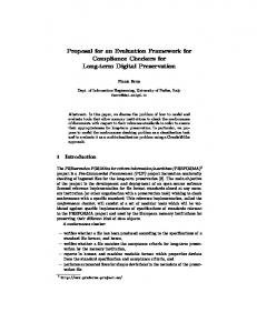
Firms - Producing Sectors The producing sectors need intermediate inputs as well as inputs of the factors capital and labor in order to produce consumption goods. They can restrictedly substitute between the different input goods. In case a good gets relatively more expensive during a model run, they can use more inputs of another good instead. The structure of inputs and the ability to substitute between those inputs to production is different for each sector, and is illustrated in detail below. As can be obtained from figure 2.1, the input structure resembles an inverse tree. The lowest end of each branch represents an input good; the entries at the crossroads represent bundles of the input goods. Each pair of branches represents a possibility of substitution between the goods to the left and to the right, i.e. shows which inputs can be substituted for each other. The elasticities next to the branches represent to what extent the input factors can be substituted for each other. A low (zero) elasticity means that there is little (no) substitution possible, whereas a higher elasticity implies a better possibility for substitution. In this nesting structure, output Y is a composite of imported goods (IM P ) and a nest of capital (K), labour (L), energy (EE) and material (M ), KLEEM , where the sectors can substitute with the elasticity σIM P . This means that a good can either be produced domestically or imported, which essentially is a reduced form of the Armington assumption (see Armington, 1969, [1]). In the next step, there exists a possibility of substitution between a capital and labour composite (nest KL) and an energy and material (EEM ) nest for domestic production with the elasticity σklem . Then again, in the different nests, the sectors can substitute between capital and labour (nest KL, elasticity σkl ), and between the energy composite (nest EE) and the material composite M with the elasticity σeem . On the bottom level, the sectors can choose between

23


different material inputs, either between electricity ELE and fossil energy EN in the energy domain (nest EE, elasticity σEE ), or between sectoral goods in the material nest M , with the elasticity σleo . The material nest is usually chosen as a Leontief-Nest (zero possibility of substitution), or with a low elasticity of substitution. Figure 2.1: The Nesting Structure of Producing Sectors

Output = Y

IMP

σimp

KLEEM σklem

KL

K

σkl

L

EEM σeem

EE

σleo

σeleen ELE

M

EN

AGR

...

SERV

The firms minimise their costs subject to CES functions, which tell us the price-dependent use of factors and intermediate inputs for each sector (see Böhringer, Rutherford, 2008, [5, p. 581]). This intuitively means that the market value of the inputs has to equal the market value of the outputs (with simultaneous market clearance, which is ensured by the market clearance conditions). Thus, within the model the sectors determine the prices of the produced goods, since the zero profit conditions imply that production costs equal net of tax consumer prices, and therefore all sectors minimize production costs by substituting between inputs. They do this subject to the constraints that all produced goods have to be sold, and that consumption demand has to be satisfied in the economy, which is guaranteed through the market clearance conditions. This can be written as

Y Πt,i (unit profit of macro sector i at time t) = pYt,i (output price of good)

− unit costs (market value of inputs for unit production) ≤ 0, The structure of the zero profit conditions described in the following will follow this pattern. These CES functions are similar to the ones described in the previous section, given in calibrated share form. However, as we use unit profit functions, benchmark levels do not have to be considered for normalisation, and we can solely rely on prices and benchmark value shares for the representation of the zero profit conditions. The functional form for the unit costs follows that presented in equation (2.30).

24


The zero profit condition for the macro sectors (excluding energy and electricity), now, reads as follows:

Y Πt,i = P Yt,i − total unit cost ≤ 0 ⇔

ηimpt,i · P IMt + (1 − ηimpt,i ) ·

1−σklemi

θklemi · KLcompt,i

(1 − θklemi ) ·

+

1−σklemi EEM compt,i

1 1−σklem i

≥ P Yt,i (2.31)

where P Yt,i

is the output price of the sectoral good

P IMt

is the fixed world market price of the good

ηimpt,i

is the endogenous share of imports

θklemi

is the share of the capital and labour composite in total sectoral production

1 − θklemi

is then the share of energy, electricity and material in total production (as all shares add up to one)

KLcompt,i

is the composite of capital and labour as shown in figure 2.1

EEMt,i

is the composite of energy, electricity and material (intermediate inputs) as shown in figure 2.1

σklemi

is the elasticity of substitution between the composites described above is the associated complementary variable

Yi

The composites themselves, now, are of all of CES, analogous to the top next and according to the nesting structure given in 2.1. Representative Household We assume an infinitely lived representative household (agent) in our model representing the population of the country. That agent is endowed with capital and time, two factors that he offers to the production sectors in return for income. We further assume that the household spends all of that income on consumption and taxes. The utility function of the household is an intertemporal composite of utility from consumption of goods and consumption of leisure. In each period the household is able to substitute between utility from these components, depending on which of them is more valuable to him at that point. Within the consumption composite of the produced goods, the household can also substitute between the single goods. The details of the substitution possibilities are displayed in the illustration below (see figure 2.2). On the top levels, households decide whether to consume energy goods or the sectoral goods with the elasticity σc . Then, on the levels below, they can decide between the sectoral goods

25


themselves, with a uniform elasticity σcy , and how they form their energy goods composite, where they choose between electricity and fossil fuels, with an elasticity σceleen . Figure 2.2: The Nesting Structure of Household Consumption

Utility σcf = calibrated Consumption

Leisure

σc

Sectoral Goods

AGR

σcy ...

Energy Goods σceleen

SERV

ELE

EN

The household can also substitute between utility today and utility tomorrow depending on an intertemporal elasticity of substitution. The utility function of the representative agent according to the above tree branch illustration reads as follows:

"

Π

W

≤0⇔

X t

P CLSt θwclst · preft

1 1−σt # 1−σ t

(2.32)

≥ PW

where is the intertemporal profit function of household welfare

ΠW

θwclst is the share of household welfare obtained in time t P CLSt is the price of full consumption including leisure at time t is the price reference path, a discount factor that is applied

preft

to all prices in the economy (exponentially) σt

denotes the intertemporal elasticity of substitution of the household

PW

is the intertemporal price of welfare

W

welfare is the associated complementary variable

Utility in each period is specified as:

ΠtCLS ≤ 0 ⇔ "

θclsc · P Ct1−σcls + (1 − θclsc ) · P LSt1−σcls

# 1−σ1

cls

≥ P CLSt (2.33)

where θclsc

26

is the share in consumption in the consumption and leisure composite


P Ct

is the price of consumption

σcls

is the elasticity of substitution between consumption and leisure

P LSt

is the price of leisure

P CLSt is the price of full consumption including leisure CLSt

full household consumption including leisure is the complementary variable

According to this the household decides how much labor she offers to the production sectors depending on the real wage rate and on the level of consumer prices. If wages are low and prices are high, she will substitute utility from consumption of goods with utility from leisure, and spend more time on free time than on working. If wages are high and prices are low she will provide more labor to the firms in order to have more income and more utility from consumption. Energy Sector As the focus of the model is put on fossil energy production, and here, at least for the Austrian economy, imports of fossil fuels play a major role, the production structure of energy sectors is organised differently, as shown in figure 2.3. In the following, when the term energy is used, it is meant as a synonym to fossil energy products, unless explicitly defined otherwise. Figure 2.3: The Nesting Structure of Energy Production

Energy

Imports

FLYE σf lye FL σf l Capital Labour

YE

AGR

...

SERV

ELE

EN

The sectors decide on the top level whether to produce fossil energy domestically (FLYE), or whether to import refined energy products (Imports). On the next level, a composite of labour and fossil fuel imports (FL) can be substituted for inputs from other sectors (YE), including energy and electricity with the elasticity σF L . Fossil fuel imports and labour can be substituted for each other with a (low) elasticity σF L . In this nesting, the imports of fossil fuels substitute for capital in the FL nest. This means that labour and raw energy can be combined, with a certain (low) elasticity, into a composite, which can then be refined using the products and inputs from other sectors (YE). Thus, the technical process of refining fossil energy is depicted by using a raw-energy - labour composite and inputs from other sectors. This technical process is held fixed in a Leontief-nest (zero

27


possibility of substitution). Also, on the top level, domestically produced fossil energy and imports are held in fixed proportions, assuming that products which are imported in a refined form cannot be substituted for domestic products in the medium term for technical reasons (no adequate refinery plants, etc.). Government Agent Apart from expenditures on the fixed bundle of consumption goods, the government agent spends money on unemployment payments, pensions and other transfers. Government income is determined by tax flows from the representative agent (labor tax, consumption tax, energy tax on households), as well as from the production sectors (energy tax on firms). The decision of the government agent is to adjust the exogenous taxes in the right way in order to make sure that government income equals expenditures. This is especially very important in the counterfactual scenarios; subsidies of different sectors work via public subsidies of consumption goods produced in these sectors. The government agent then raises taxes in order to refinance these expenditures. Bottom-Up: The Electricity Sector In the presented model, the electricity sector is divided into seven technologies, hydro power, wind, solar, biomass, coal, oil and gas, all of which produce electricity subject to different input structures, resource constraints and production costs. In total, aggregate produced electricity has to meet consumption demand for electricity. The mathematical description of the problem is given in section 2.1.2. The different technologies have different production costs, but there is a unique market price for electricity that is determined by the production cost of the most expensive technology. If the cheap technologies produce enough output to meet demand, the more expensive technologies will not be active. But since the cheaper technologies underlie different constraints, namely equation (2.13), also the more expensive technologies produce at a positive level. The difference between production costs and revenues (i.e. the profit that arises for some cheap technologies) is being paid to the households, and can be interpreted as rents on natural resources and capacities. This makes simultaneous modelling of different technological production costs and a unique output price of electricity possible. The complementarity conditions between Lagrange multipliers and constraints can be exploited to solve the linear problem together with the top down macroeconomic equilibrium of the overall economy. This is done by including the market price for a unit electricity pele , the shadow price on the capacity constraint pcap and the shadow price of on the resource constraint pr as additional variables and by adding equations (2.12) and (2.13) as additional zero profit or market clearance conditions.

28


Model Mechanics Based on the SAM and on additional input data like for instance estimated interest, depreciation or growth rate, a calibrated equilibrium path from 2005 until a specified time period in the future, such as 2030 or 2050, is developed. This path is merely a mathematical representation of the model, the so called benchmark, while the realistic future development is calculated in a model run with realistic constraints, for example on resources, and capacities. This new realistic equilibrium path solution is referred to as the business as usual (BAU) scenario, indicating a possible future development without any changes in political or environmental circumstances. In the counterfactual scenarios one usually analyses the effects of political interventions changing the initial economic circumstances, comparing the results to the BAU scenario. As an example of a counterfactual scenario we give the following: The government agent decides to gives subsidies to households to foster the penetration of electric mobility in individual transport, e.g. a feebate system on xEVs. This feebate will reduce the price of xEVs in relation to other forms of individual transport such as CVs, and therefore induce the household agent to consume more of BEVs/PHEVs. This will shift the demand for individual transport to electromobility, but might also have repercussions on the mode choice of the representative household, since the whole bundle of individual transport will become cheaper in relation to public transport. This again might have feedback effects on the macroeconomy, e.g. growth, employment and the sectoral composition of production. In order to refinance these expenditures, the government agent has to increase income by increasing taxes. The endogenous adjustment of all different taxes is possible within the model. The overall effects of the political actions presented here depend greatly on the height of subsidies, the duration of subsidies, the tax instrument used to refinance the spending, and the decision which sectors to subsidize.

29

CHAPTER

3

Model Extensions in DEFINE

3.1 Extentions to Standard Austrian I/O Tables The reference for the SAM constructed for the IHS CGE model to be used for cost estimation in DEFINE was Table 40 of Austrian I/O Tables for the year of 2008 (IOT 2008)1 . Other sources as compared to the two-digit I/O Tables for 2008 were Austrian I/O Tables of 2007 (see table 3.1, I/O Tables 8, 16), as some tables with the higher sectoral disaggregation necessary for the model dataset were not published any more in 2008, as well as the structural business statistics (SBS) by Statistics Austria.2 . Table 3.1: National Accounting Data by Statistics Austria used for DEFINE

IOT 2007 Table Table Table Table

8 Intermediate consumption at purchasers’ prices (73 products x 73 industries) 16 Final uses at purchasers’ prices (73 products) 44 Input-output table at basic prices, domestic output 43 Input-output table at basic prices, domestic output and imports

IOT 2008 Table Table Table Table Table

37 39 40 41 42

Final consumption expenditure by households CPA x COICOP Employment (Products) Input-output table at basic prices, domestic output and imports Input-output table at basic prices, domestic output Input-output table, imports at cif-prices

SBS - Structural Business Statistics for Austria Structural Business Statistics 2007 Structural Business Statistics 2008 The SBS dataset provides information with a much higher sectoral detail than the one of the Austrian I/O tables that only feature 75 sectors. Thereby, sub-sectors such as wholesale

1

2

30

For further information, see http://www.statistik.at/web_en/dynamic/statistics/national_ accounts/input_output_statistics/publikationen?id=&webcat=358&nodeId=1096&frag=3&listid= 358. Or “Leistungs- und Strukturdaten” (LSE) in German, see http://www.statistik.at/web_en/statistics/ industry_and_construction/structural_business_statistics/index.html.

3.1 Extentions to Standard Austrian I/O Tables

of vehicles and vehicle maintenance, repair, etc. could be identified and disaggregated. The following sub-sectors were used to disaggregate IO Sectors given in the Austrian IOT (see table 3.2, classification ÖCPA 20083 ). The aggregation for the IHS CGE model developed in DEFINE can be obtained from table 3.3. Table 3.2: Sub-Sectors of Austrian National Accounting Data Used for Disaggregation (including Source)

Source

(Sub-)Sector Number, CPA

Name of Sector Disaggregated Using Austrian National Accounting Data

IOT2007

04

Coal and peat

IOT2007

05

Crude petroleum, natural gas, mineral ores

IOT2007

06

Rest of sectors 05-09

IOT2007

35.1

Electricity, transmission and distribution services

IOT2007

35.2

Manufactured gas; distribution services of gaseous fuels through mains

IOT2007

35.3

Steam and air conditioning supply services

IOT2007

45.2

Maintenance and repair services of motor vehicles

SBS2008

Rest 45

Rest: Wholesale- a. retail trade, repair of motor vehicles

SBS2008

47.3

Retail trade services of automotive fuel and other new goods n.e.c.

SBS2008

Rest 47

Rest of Retail trade, exc. o.motor vehicles a. -cycles

SBS2008

49.1, 49.3

Land transport services: Passenger transport

IOT2007, Rest 49 SBS2008

Land transport services a. transport services via pipelines: Freight transport

SBS2008

50.3

Water transport services: Passenger transport

SBS2008

50.4

Water transport services: Freight transport

SBS2008

51.1

Air transport services: Passenger transport

SBS2008

51.2

Air transport services: Freight transport

SBS2008

77.1

Rental and leasing services of motor vehicles

SBS2008

Rest 77

Rest of Rental and leasing services

Another important data source, especially for tax revenue by the government and government transfers, was tax revenue and government expenditure data by Statistics Austria (henceforth referred to as Tax Data).4

3 4

For more information on the classification of Austrian I/O tables, see e.g. http://www.statistik.at/web_ en/classifications/implementation_of_the_onace2008/index.html. For further informatio on this national accounting data, please see http://www.statistik.at/ web_en/statistics/Public_finance_taxes/public_finance/tax_revenue/index.html (English version, less detail) or http://www.statistik.at/web_de/statistiken/oeffentliche_finanzen_und_steuern/ oeffentliche_finanzen/steuereinnahmen/index.html (German, more detail).

31

3 Model Extensions in DEFINE

Table 3.3: Sectors of 2008 SAM for DEFINE

Abbreviation

Sector Name

CPA 2008 Sectors/Data Source

AGR FERR

01, 02, 03 24

PUBTRANS PPT FT R&D SERV

Agriculture Ferrous, Non-Ferrous Ore and Metals Chemical Products Engineering Car Production and Trade Conventional Vehicles Hybrid Electric Vehicles Plug-in Hybrid Electric Vehicles Battery Electric Vehicles Other Vehicle Prod. Other Production Buildings and building construction works Constr. and constr. works f. civil eng. Public Transport Private Passenger Transport Freight Transport Research and Development Services

CARSERV ELPRO ELTD DH GASTD COAL OILGASCOKE FUEL OWNINT U-LS, SU-LS, RLS U-MS, SU-MS, RMS U-HS, SU-HS, RHS IMP K LTAX KTAX PENSION MoeSt

Car Services Electricity Production Electricity Transm. and Distr. District Heating Natural Gas Transm. and Distr. Coal Oil, Gas and coke Fuel for Transport Purposes Intermediate Inputs within Sector Urban, Suburban, Rural Low-skilled Labour Urban, Suburban, Rural Mediumskilled Labour Urban, Suburban, Rural High-skilled Labour Imports Capital Labour Taxes Capital Taxes Pension Benefits Mineral Oil Tax

CONSTAX

Consumption Tax

INTTAX UEBEN OTHTRANS

Taxes on Production Unemployment Benefits Other Social Transfers

CHEM ENG CPT CV HEV PHEV BEV OVEPRO OTHER BUI1 BUI2

32

20, 21 25-28, 33 29, 45.1, 45.3 Own calculations Own calculations Own calculations Own calculations 30 rest 05-09;10-18, 22-23, 31-32, 58 41, 42 43 49.1, 49.3 50.3, 50.1, 51.1 49.2, 49.4, 49.5, 50.4, 51.2 72 36-39, 45.4, 46-47 excl. 47.3, 52-53, 55-56, 58-66, 68-75, 77 (excl. 77.1)82, 84-88, 90-97 45.2, 47.3, 77.1 Part of 35.1. Part of 35.1. 35.3 35.2 5 6, 9.1, 19 except fuel Own calculations I/O Tables I/O Tables/EU-SILC I/O Tables/EU-SILC I/O Tables/EU-SILC I/O Tables I/O Tables/EU-SILC I/O Tables/EU-SILC EU-SILC/Tax Data Tax Data/EU-SILC data I/O Tables (fuel consumption, table 37)/official tax rate I/O Tables (total consumption)/official tax rate Tax Data Tax Data Tax Data

3.2 Mobility Good - Disaggregation of Transport Sector

3.2 Mobility Good - Disaggregation of Transport Sector The most important changes regarding the transport sector are: • The four modes of individual transport are modelled as separate goods (CV, HEV, xEVs) that are purchased by the household sectors, but take as input – the chassis and internal combustion engine (CV, HEV) from the car production and trade sector – battery/engine (PHEV) and battery (EV), respectively, from the engineering sector – car services from a car service sector – fuel (diesel, gasoline, gas, LNG) from a separate fuel sector in the case of CVs, HEVs, PHEVs (part of fuel input), electricity (for PHEVs in relation to electrically powered car use) in case of xEVs • The engineering sector was split up into production of other vehicles (OVEPRO), as well as into a car production sector, where car trade was added in from the service sector to construct a car production and trade (CPT) sector, and finally into a remaining part constituting the rest of the engineering sector (ENG). • The transport sector was split up into public transport (PUBTRANS), private passenger transport (PPT) and freight transport (FT). In the logic followed in this model, the households can decide on the transport mode (public or individual transport) as well as the technology/fuel used for their individual transport means (CV, HEV, xEV). Therefore, it was important to distinguish between public transport (PUBTRANS) that could act as a substitute for individual motorized transport by car (IT), and other private passenger transport (PPT) such as airplanes or water transport that are no substitute for IT. Here, again, data from the structural business statistics werde called on to disaggregate the respective sector.

3.2.1 CV, HEV, xEVs as separate goods A particular challenge was to introduce different vehicle types into the model distinguishing between conventional vehicles (CVs) and different modes of alternatively fuelled vehicles (HEVs, xEVs). Since, unlike above, data on these issues are not available from national accounting or any other data provided by Statistics Austria, several sources of information were used to find the present share of different vehicle types for both stock and new purchase of these car types. The following data sets were used: • New Registrations of Cars in Austria (Statistics Austria5 ) 5

http://www.statistik.at/web_de/statistiken/verkehr/strasse/kraftfahrzeuge_-_ neuzulassungen/

33


• Existing Vehicle Stock in Austria (Statistics Austria6 ) • Data on share of engine/battery in total vehicle costs: Haas et al. (2009, [21]), data from the Fraunhofer Institute for Manufacturing Technology and Advanced Materials (IFAM)7 , Crist (2012, [14]), as well as expert data input from DEFINE project partners TUW, UBA and OEI. The disaggregation strategy for the different types of alternatively fuelled vehicles was as follows: it was assumed that, largely, the chassis and other components have the same costs for all different car types. The only major difference would lie in the input costs for the different types of engine (conventional or electric) and, most importantly, in the different (higher) costs for batteries for electrified vehicles. Accordingly, the cost share of the engine (CVs, HEVs) and the battery (xEVs) were calculated in relation to the total costs of the vehicles, and the input structure for CVs, HEVs and xEVs, i.e. the input share between the car production and trade and the rest of the engineering sector, was adapted accordingly. Thus, production of these vehicles has a different input structure, since the proportions between the monetary value of the chassis and the one of engine and/or battery, as well as the sector providing the input, may be different for all car types. Furthermore, naturally, the car types use different fuels: CVs (and HEVs) take input from an especially constructed fuel sector, xEVs use electricity. All vehicle types take as an input a fixed share of service and maintenance from the car service sector (CARSERV), which is identified using the SBS. The share of new purchases by car type was calculated according to the cars bought in the reference period, i.e. new registrations 2008, and fuel input according to the total existing stock of vehicles Structure of Mobility Good CV and xEV sectors are different from other sectors of the model economy: they do not take any input except for that of the car production and trade, the engineering, car service, fossil fuel (CV, HEV, PHEV), electricity (xEV) sector, and pay a specific tax on fuel consumption (mineral oil tax). Therefore, it rather reflects the use of a vehicle type rather than its mere purchase. There is no input of other sectors/factors such as capital, labour, imports, etc., of any kind for these goods. Much of the sectoral economic structure relevant for assessing the shift to electromobility is reflected by the sectors that provide the inputs for the different car types. The reason for this construction is the following: we explicitly see the different car types as technology, where we assume a fixed share of production (Leontief-technologies). This means that the consumer who buys the car is confronted with a fixed share of fuel, car service, electricity, etc., which can only be changed exogenously. Thus, we are able to model scenarios such as fuel efficiency, the impact of additional mineral oil taxation on car purchases and mobility behaviour, and the like. The corresponding new

6 7

34

http://www.statistik.at/web_de/statistiken/verkehr/strasse/kraftfahrzeuge_-_bestand/index. html System Research for Electromobility, see http://www.elektromobilitaet.fraunhofer.de/en.html


nesting structure of household consumption corresponds to the one shown in figure 3.1.

35

36 Figure 3.1:

New Nesting Structure in Consumption separately including Mobility Goods Consumption σ T RAN S Mobility Goods Composite

σ cst Car-Substitutable Non-car Substitutable

Non-Mobility Goods Composite

Sec 1 . . .

σc

. . .N

σM C IT

PUBTRANS

CV, HEV Use

EV Use

0 (Leontief) CV,HEV

OIL

SERV

EV

PHEV Use

0 (Leontief) 0 (Leontief) ELE SERV PHEV OIL, ELE SERV Source: IHS 2013


σ IT


3.2.2 Household Individual Transport Demand - Modelling Methods This section is specifically concerned with how to model household demand for different vehicle types, which is the focus of the DEFINE project regarding CGE modelling. At the first DEFINE technical modelling workshop in November 2012, several approaches to model this (rising) household demand for electromobility were discussed and assessed. These are presented in short, and the choice made for DEFINE is explained. Generally, the goods CVs, HEVs and xEVs are not modelled analogously to the other sectors of production here, but rather as what one might call "consumption-structures": they only take intermediate input from the car production and trade sector (the chassis), the engineering sector (engine and/or battery), the car services sector, and fuel from the separate fuel sector and/or from the electricity sector (see section 3.2 above), but use no other intermediate input, factor of production, or directly imported goods. Therefore, the input structure for these different vehicle types is rather reflected in the sectors providing intermediate inputs. Constant-Elascity-of-Substitution (CES) Functions CES utility/expenditure/demand functions are the standard approach in CGE modelling (see section 2.2.2). An exogenously specified, fixed elasticity of substitution governs the reaction of consumers to changes in relative prices of goods. Its advantages are easy implementation within the model, and a smooth substitution behaviour between goods that are already present beginning from the first model year. Disadvantages However, CES functions have their weaknesses when it comes to analysing the introduction of goods that start with low initial shares in consumption demand in the benchmark year. The expenditure function of the household in calibrated share form has a functional specification analogous to the one shown in Equation (2.30).8 As one can see from this functional form, it follows that the benchmark share of a certain good in consumption (the θi ) matters greatly for policy scenarios in the model: if the benchmark share for a good is very low, as it is the case especially for xEVs in the benchmark year 2008 (less than 0.1 %), even if the respective (constant) elasticity of substitution is very high, it will require very large price shifts to introduce xEVs in a larger scale. This might produce unrealistic cost estimates, which certainly is not a desirable modelling feature. Goods that are not present in the benchmark dataset cannot be analysed at all, since they cannot be shifted into the production structure of sectors and the consumption patterns of households, respectively. Therefore, at the first technical modelling workshop, two alternative modelling approaches, their implementation as well as their advantages and disadvantages were discussed. They are presented in the following. 8

The only difference being that the relative differences of benchmark good prices are considered instead of relative benchmark input prices, and that benchmark expenditures are used as scaling parameter instead of benchmark costs. See also Böhringer et al. (2003, [6, p. 10]).

37


Homogenous Goods Modelling different vehicle types as homogenous goods assumes the following features: • Different transport modes are perfect substitutes, and • the characteristics only depend on the price level. In this setting, the differenct vehicly types can be thought of as different "technologies" used to "produce" a homogenous good with undistinguishable characteristics (think of electricity as an example). To control how quickly a technology enters in the production process of this homogenous good can be achieved in the following way: • Setting lower and upper bounds for the technologies (think of production capacities of power plants to produce electricity), and/or by • calibrating a fixed factor to model a supply elasticity (think of a factor that is fixed in production, such as land). This means that the more you produce of a good, the more expensive its production becomes due to the relative scarcity of the fixed factor of production. This renders technologies, who may be cheaper than others up to a certain volume of production, more expensive than other technologies for higher levels of production. To put it differently, since for all technologies the exogenous amount of the fixed factor they have to use for their production process is potentially different, they each may exhibit different supply elasticities. Here, a step-wise supply function with upper and lower bounds would mean very rough changes in the provision of the good. For example, a raise in the price of PHEVs so that it becomes more expensive than all other vehicle technologies would mean that all other car technologies are used before PHEVs to produce the homogenous transport good up to their respective capacity constraints (since they are perfect substitutes!). This might not be a very realistic depiction of a market as complex as the vehicle market, especially since we are dealing with vehicle stocks here. Kick-in kick-out (bang-bang) solutions are not a very good option here, since the use of a vehicle stock will exhibit a high amount of inertia in relation to the stock itself. Supply and cross-price elasticities calibrated with a fixed factor, on the other hand, would allow for a much smoother introduction of a new car technology from the supply side. The interpretation of this could be that fixed factors of production (such as car factories primarily designed for producing conventional cars) render the production of alternative vehicle types such as xEVs in regard to higher sale volumes more expensive in the short and medium run as compared to their more conventional competitors. This would slow down their widespread introduction in the vehicle market. One might also use a combination of these two methods to control the introduction of alternative vehicle types in a reasonably realistic fashion to replicate the results of the vehicle stock projections from DEFINE partners UBA (Austria) and OEI (Germany). Considering

38


the competition between new and old technologies, whereby the new technologies would have higher initial investment costs (to erect new car factories etc.) than more conventional technologies, this seems like a reasonable modelling procedure which could provide more realistic cost estimates than CES consumption functions However, the richness of information on heterogeneity of the different vehicle types in view of consumer preferences obtained from the household survey conducted in DEFINE WPs 3 and 8 would cannot be realized in a full extent within this modelling approach. Logit A third solution considering the heterogeneity of goods and household preferences along several dimensions by using a logit demand function was mentioned during the first DEFINE modelling workshop. After careful consideration and initial research effort, this approach was chosen, in spite of the facts that it was not initially foreseen in the consortium plan and considerably increases the workload especially for DEFINE WPs 1, 6 (CGE Modelling), but also for WPs 3, 8 (Household Surveys and Micro-Data for Austria and Poland, respectively). This approach appropriately addresses the modelling challenges as laid out in section 1.2, and allows to include a large proportion of the richness of the micro-data obtained on heterogenous household preferences within the household surveys. Implementation in CGE Model The main idea is to include a microeconometrically estimated discrete choice model, aggregated to the amount of household detail featured in the CGE model (9 households, see section 3.3), directly within the CGE framework. Demand for different vehicle types (CVs, HEVs, xEVs) is taken from a multinomial logit model depicting the choice probabilities of certain household types dependent on car purchase and fuel prices, socio-demographic characteristics, as well as the technical charecteristics of the car technologies (range, power, infrastructure availability, etc.). The main challenge here was to derive an aggregate price for the bundle of car technologies (individual transport nest in household consumption, see figure 3.1) dependent on prices and technological attributes of the car technologies, as well as on socio-demographic characteristics of the household types following Truong and Hensher (2012, [45]). An indirect utility function is derived incorporating the information obtained from the household survey, and the choice probabilities from the logit model interpreted as market shares are used to derive household demand for the individual car types. Overall demand for individual transportation is obtained from the aggregated indirect household utility of individual transport as a composite of the single car types, interpreted as an aggregate price or willingness-to-pay, in relation to substitution possibilities in the consumption bundle, such as public transport. The detailed hard link between MERCI and results as well as estimations from the household survey of WP 3 is currently under construction and a preliminary version has already been implemented successfully in the model. A draft version of a paper on this link was already

39


presented by Stefan Schmelzer and Michael Miess at the top-down bottom-up talks at the DIW in Berlin at the end of November 2013. This micro-macro link enables the above-mentioned direct integration of heterogenous household preferences and different technical characteristics into household demand for the specific vehicle types. Details on the implementation and construction of this link will be made available in the first DEFINE Working paper soon9 . Progress beyond State-of-the-Art It clearly has to be stated that this modelling approach transgresses the state-of-the-art in CGE modelling, as the authors are aware of no model that has implemented this approach regarding vehicle purchase choice for Austria, Germany or Poland. Furthermore, the combination with technological detail from the electricity sector obtained from the large-scale bottom-up electricity market models of DEFINE partners TUW and DIW, and incorporating detailed vehicle stock projections stemming from separate modelling tools available to DEFINE partners UBA and OEI, makes the approach taken in DEFINE unique. First simulations with a preliminary and simplified version of the micro-macro link show encouraging results, especially as regarding to changes in the technical characteristics (e.g. range) of car technologies. With this approach, technological progress can be assessed in relation to heterogeneity of household preferences, which certainly is a very desireable feature for the type of analysis conductedn in DEFINE.

3.2.3 Disaggregation of Engineering Sector and Transport Sector The sector motor vehicles, trailers and semi-trailers (29) is provided as a separate sector in the Austrian I/O tables. For modelling reasons, however, it was decided that trade of vehicles should be integrated with their production into one sector. The intuition behind this from the viewpoint of a CGE model is quite simple: for the consumer, buying a new vehicle involves a purchase decision where he/she cannot distinguish between the production costs and the commercial margin charged by the car trader. Rather, the consumer will decide on a price that will always incorporate both of these elements. Since for a CGE model one has to assume one representative good depicting all car dealers and all car manufacturers at once, aggregating these two sectors definitely corresponds to the logic of a CGE model. To disaggregate the engineering and transport sector, and to isolate trade of vehicles, the structural business statistics by Statistics Austria had to be used. Thereby, sub-sectors such as wholesale of vehicles and vehicle maintenance, repair, etc. could be identified and disaggregated. However, the structural business statistics only report on employment, value added, production value, investment, aggregate intermediate inputs, etc., of these sub-sectors, even though in very high detail. Unlike I/O tables, the linkages and monetary flows between sectors are not 9

40

Available on the DEFINE project homepage, see http://www.ihs.ac.at/projects/define/ under "Recent Deliverables" or under http://www.ihs.ac.at/projects/define/scientific-debate-1.html.


considered. Thus, one has to make the assumption that the input-output structure remains the same for both newly disaggregated sectors, and uses the aggregate intermediate inputs, wage, total value added, etc., figures of the structural business statistics for each sub-sector as assistance and control variables to split up the aggregated I/O transport sector. Since the respective sub-sectors should be quite similar on this level of detail as regarding inputs they require from other sectors, this assumption seems reasonable. What rather matters in this context is the real price for vehicles to be paid by the households, which can be addressed by this method.

3.2.4 Construction of Fuel Sector - Electricity Input for xEVs In order to explicitly account for fossil fuel input for CVs, HEVs and also PHEVs (for mileage not covered with electric energy), a fuel sector had to be carved out of the I/O sector for coke and refined petroleum products (sector 19 in ÖCPA 2008). This was done using the following additional data sources provided by Statistics Austria: • Energy accounts10 , • Useful energy enalysis11 , • Energy consumption of households12 , • Average annual prices for most relevant fuels13 . Firstly, coke consumption by sectors had to be separated from the consumption of refined petroleum products using the energy accounts. Secondly, the share of refined petroleum products for mobility purposes is separated from the total amount using the useful energy analysis. The input structure for the newly constructed fuel sector is assumed to be the same as the aggregated sector 19, since the same facilities (refineries etc.) are used for its production. As all of the data sets mentioned above measure in physical units, i.e. liters of refined petroleum or tons of coke, the average annual prices from statistics Austria were applied to calculate annual financial flows as depicted in the SAM. The final question then remains as to what share of total refined petroleum products is bought by households, i.e. the input into the CV consumption good in the SAM as households purchase individual mobility by car type in a bundle including the fuel. For this purpose, physical data on the energy consumption of households14 , and table 37 of the I/O data (final consumption expenditures by households) are used as reference. Furthermore, the tax

10 http://www.statistik.at/web_en/statistics/energy_environment/energy/energy_accounts/index. html 11 http://www.statistik.at/web_en/statistics/energy_environment/energy/useful_energy_ analysis/index.html 12 http://www.statistik.at/web_en/statistics/energy_environment/energy/energy_consumption_of_ households/index.html 13 http://www.statistik.at/web_en/statistics/energy_environment/energy/prices_taxes/index. html 14 Especially regarding use and mileage of cars, see www.statistik.at/web_en/static/driven_kilometres_ and_fuel_consumption_of_private_cars_by_laender_2000_to__034836.xlsx

41


expenditures on fuel (mineral oil tax) are calculated using official tax rates. Finally, the share of CVs, HEVs and PHEVs in total fuel expenditures by households is calculated according to data on the existing vehicle stock by statistics Austria and average mileages. Electricity input into xEVs was calculated as follows: Average mileage driven with electric energy by vehicle type × Number of xEVs taken from data on existing vehicle stock × Average electricity consumption in kWh × Average price of electricity used for the xEV.

3.3 Household Disaggregation On the demand side the Representative Agent was disaggregated according to three skill levels (low-, medium, and high-skilled)15 and according to 3 degrees of urbanization (urban, sub-urban, rural)16 using EU-SILC data17 , so that detailed and realistic characterization of consumer choices regarding the traffic and transportation system is met. In accordance with econometric literature (as in the spirit of Mincer, 1958, [36]), we take education as a proxy for income at this point. There are several justifications of this approach in the context of CGE modelling: • Income classes would be endogenous in the CGE model: if the level of (average) wages for different income classes changes, this might change the composition of the income classes themselves depending on the underlying household data. Incorporationg this within the CGE model seems to be either too difficult to implement without much additional insight, or plainly impossible as regarding numerical solution methods. • This approach is in line with much of the CGE modelling literature (e.g. other CGE models at IHS18 ), and thus guarantees consistency for comparison of results. • All estimates for the effect of skill level on income are highly significant in microeconometric estimates, thus making the skill level (highest education attained) a good proxy for income. • Household preferences, which might not only depend on income, but also on other sociodemographic characteristics rather refleced in the highest level of education attained, are a major factor in the vehicle purchase decision. Skill groups could be a better proxy for household preferences than income classes.

15 On ISCED classification, see http://www.unesco.org/education/information/nfsunesco/doc/isced_ 1997.htm. Low-skilled: ISCED 0-2, medium-skilled: ISCED 3-4, high-skilled: ISCED ≥ 5. 16 On DEGURBA classification, see http://ec.europa.eu/eurostat/ramon/miscellaneous/index.cfm? TargetUrl=DSP_DEGURBA. Urban: DEGURBA=1, sub-urban: DEBGURBA=2, rural: DEGURBA=3. 17 European Union Statistics on Income and Living Conditions, see http://epp.eurostat.ec.europa.eu/ portal/page/portal/microdata/eu_silc. 18 For extensive documentation for an example of this type of CGE model at IHS, see Berger et al. (2009, [3]), available at ec.europa.eu/social/BlobServlet?docId=4276&langId=en.

42

3.3 Household Disaggregation

The resulting 9 household sectors in the skill × degree of urbanisation matrix all have different income levels due to different labour and capital income shares in total national labour/capital income (both separately calculated from EU SILC data). Labour and capital taxation are taken as average rates for each household type (calculated from EU-SILC data) and applied to labour and capital income of the different household types. Furthermore, the share of each household type in aggregate social benefits such as pension income, unemployment benefits, etc., are all calculated from EU SILC data. National aggregates of these figures obtained from tax data by Statistics Austria are then disaggregated to the different household types using shares from EU-SILC. Thus, consistency with Austrian national accounting data can be achieved. Since the SAM has to balance (sums of all rows and columns, respectively, have to be equal to zero), the net income of all households has to be spent on consumption. The disposable income of households net of taxes and including social benefits determines their level of consumption. Consumption patterns across all goods were kept the same for all household types for reasons of simplicity. Value added taxes on consumption are simply a fixed share of total consumption (average tax rate across all goods) for the different household types. Only for the benchmark consumption individual transport represented in the SAM (CVs, HEVs, xEVs) heterogenous consumption shares are assumed for the different household types. Consumption of IT is distributed among the 9 household types according to the household data survey conducted in WP 3. Furthermore, household preferences regarding the consumption of mobility are assumed to be heterogeneous, especially when it comes to vehicle purchase choice in relation to electrically fuelled cars. Details on this matter are elaborated on in the next subsection.

3.3.1 Elasticities In DEFINE, a data survey and micro estimation provide sufficient empirical support for the CGE model. There are two separate surveys, which were either already conducted (Austria, WP 3) or are in the process of being conducted (Poland, WP 8), that should, at least, provide different elasticities for CES utility functions as regarding transport mode choice (public transport vs. individual motorized transport, i.e. cars) and as regarding vehicle purchase choice (CVs, HEVs, xEVs) for all 9 household types described above. Currently a stylized hard-link between the CGE model and an aggregate version of household survey data from WP 3 is under construction. This might make a more detailed depiction of heterogeneity in household preferences as well as more realistic scenarios for the introduction of electromobility possible. As of yet, however, it is still work in progress, and will be further described in the next DEFINE working paper.

43


3.4 Electricity Sector 3.4.1 Intermediate and Factor Input Structure In order to arrive at a suitable electricity sector in the top-down bottom-up framework, it was necessary to distinguish between electricity production proper (sector ELPRO), i.e. the actual production of electricity in power plants/via different technolgies, and electricity transmission, distribution and trade (sector ELTD). For this, again the Structural Business Statistics for Austria were used. Input and Cost Structure Furthermore, the intermediate and factor input structure for the different electricity technologies had to be calclulated. Of course, factor and intermediate inputs (capital, labour, other sectors) for the distinct technologies in total have to sum up to intermediate and factor inputs of the electricity production (ELPRO) sector in total, the sum of electricity supply of technologies should correspond to total production of the ELPRO sector. A variety of sources was used to calculate these data, so that investment costs could be annualized and added to the capital account, and operating costs separated from investment costs, among others. Technologies The following electricity producing technologies were introduced, many of them new in the model, and all of them with an extended and updated database to determine its sectoral input structure, investment (capital) and labour costs, and the costs of electricity production measured in monetary terms per unit of electricity produced: Wind Onshore

Photovoltaics

Pump Storage Hydro

Run of the River Hydro

Biomass solid

Biomass liquid

Biogas

Geothermics

Landfill and Sewage Gas

Bituminous Coal

Natural Gas

Oil

Lignite

Nuclear Energy

Sources Among others, the sources employed to estimate the input structure of technologies are: • Schröder et al. (2013, [43]) • Biermayr (2009, [7]) • Bodenhöfer et al. (2004, [9], and 2007, [8]) • E-Control Austria (2009, [17], 2010, [18], 2012, [19]) • Lang and Rohrer (2011, [27]) • Data on power plants in 2008 by E-Control Austria19

19 See http://www.e-control.at/de/statistik/strom/bestandsstatistik (Only available in German).

44

3.4 Electricity Sector

• Energy Balances 2008 by Statistics Austria20 • Structural Business Statistics by Statistics Austria21

3.4.2 Incorporating Results of Detailed Electricity Market Models The CGE model, which features a very aggregated bottom-up technology representation of the electricity sector on a yearly basis, is planned to be calibrated to the results of the much more detailed electricity market models of DIW and TUW. To this end, the results of these models, which feature hourly or even higher resolution of electricity production and consumption at very high technological and geographical detail, shall be aggregated in a way that they can serve as input for the CGE model. To enter the CGE model, inputs from the electricity market models would have the following structure: • Yearly production of electricity in GWh per power plant type, • Production costs per GWh of electricity per power plant type, • Investment costs incurred for building of new power plants, • Yearly average elelctricity market price (= production costs of most expensive technology in yearly merit order curve), • Amount of subsidized electricity per year (“EEG Umlage, Ökostromförderung” in Germany and Austria, respectively). The second technical modelling workshop with Prof. Böhringer in February 2014 will, among other things, be dedicated to calibrating the CGE model to the results from the more detailed external electricity market models of DIW and TUW, e.g. by using modelling procedures for homegenous goods as described in section 3.2.2. Modelling objective: The CGE model has to deliver the same results as the much more disaggregated and specialized electricity market models of DIW/TUW on a more aggregated level. Thus, similar to the vehicle stocks (see section 3.5), the model should meet certain parameters provided by the electricity market models, among them: • Similar relative electricity price changes, • Same technology mix on a more aggregated level, • Investment costs for new power plants, • Similar subsidy rates leading to the same share of renewables in electricity production. 20 See http://www.statistik.at/web_en/statistics/energy_environment/energy/energy_balances/ index.html. 21 See http://www.statistik.at/web_en/statistics/industry_and_construction/structural_ business_statistics/index.html.

45


Investment for power plants in this context is best modelled on an annualized basis in the CGE model. The model is not really suited for big expenditures within one year or a couple of years, especially since the forward-looking representative agents in the model would anticipate the sudden increase in spending and behave accordingly. Interaction between Electromobility and Electricity System in CGE Model The aim of incorporating the electricity sector into the CGE model is the assessment of costs and savings for the energy system induced by introducing electromobility on a broader scale. Possible components of this cost-benefit analysis are e.g. the following: • Costs of producing additional electricity to satisfy demand of EVs, PHEVs, including investment costs into new power plants, • Savings in building new power plants because EVs, PHEVs can serve as storage technology (also in connection to an increased share of renewables in electricity production, “Energiewende” in Germany and Austria), • Savings by less imports of fossil fuels (e.g. gasoline, diesel) due to reduced use of CVs, HEVs, • Infrastructure costs incurred for the introduction of electromobility, e.g. grid investments (extensions, smart grids), charging stations for EVs. etc. EV/PHEV Feedback into Electricity Production In principle, EVs/PHEVs could feedback into electricity production during peak load times and act as an additional sink during periods of high electricity production: vehicle to grid (V2G) solutions. V2G may not pay off economically considering the current technological circumstances, mostly because of increased battery degradation due to discharging the battery during peak load times without using it for mobility purposes. TUW is in contact with leading researchers in this area, and will deliver input as to what extent V2G is a viable future option and whether it will enter electricity market modelling. In the bottom-up part of the CGE model, it will probably not be meaningful to explicitly include V2G concepts because of the following reason: • V2G is not really an electricity-producing technology: Yearly aggregation reduces the net quantity effect of input22 and output to zero, even though V2G concepts might alleviate the burden on the electricity system by smoothing peaks in production (irregular feed-in by renewables) and consumption. If, however, V2G solutions enter the detailed electricity market models, this will most likely change electricity prices and the technology mix, among others. Thus, as the CGE model is intended to be calibrated to the results of the electricity market models, the economic effects of V2G solutions would be assessed on an aggregated, annual scale. 22 Entering as a negative number.

46

3.5 Calibrating the CGE Model

3.5 Calibrating the CGE Model CGE model will have to replicate two exogenously given reference paths: • Vehicle stock projection by UBA/OEI, • Electricity producing “technology mix” (DIW/TUW), together with the corresponding price level. • Additonally, the increase/decrease of energy consumption by vehicle type has to be explicitly considered in electricity production and fossil fuel imports. Corresponding model variables and parameters have to be set accordingly to meet these exogenously given values in the Business As Usual (BAU) run. For further analysis, the BAU will serve as the reference path for all policy scenarios, in relation to which all cost estimates are given. As all policy recommendations and conclusion will be based on the relative difference between the BAU and the policy scenario, this procedure will decisively determine the results of DEFINE. Therefore, this matter should be handled with great care and will be discussed using expert inputs. To replicate vehicle stock projections, tax instruments as proposed in scenario development by partners UBA/OEI (see section 4.1) have to be used accordingly to reach the BAU as well as the emob+ policy scenario. Careful consideration of what instrument should be used to what extent have to be taken in order to achieve a sound analysis. As regarding the requirement for the CGE model to replicate the price and quantity developments calculated in the electicity market models, this places an addional constraint on the bottom-up electricity sector of the model. This might raise computational and methodological issues. Workshop Calibrating the model to these exogenous reference paths will be discussed, among other topics, in the second DEFINE CGE modelling workshop with Prof. Christoph Böhringer from the University of Oldenburg, which is scheduled to take place in February 2014.

47

CHAPTER

4

Applicability of Improved Model to Modelling Challenges

4.1 Modelling of Measures for Electromobility At the DEFINE scenario workhsop in April 2012, several measures were defined that should be depicted in the CGE modelling framework. The ranked results of discussion among partners (rank according to support of individual measure by members of scenario workshop) are the following: 1. Tightening of CO2 -regulation 2. NoVA1 , feebate system 3. Fossil fuel price paths (mostly set by adapting mineral oil tax) 4. Service station expansion 5. Awareness building 6. Subsidy battery costs 7. Financing of measures for emobility by dedicating tax revenues (e.g. mineral oil tax) and privilege for emobility in urban transport (parking, lanes, etc.) 8. Privilege for public transport The extensions of the core CGE model are designed in such a way so that all of these measures can be depicted appropriately. As far as can be judged at the present moment before the actual process of modelling and calibration, these measures could be simulated in the model according to the following paragraphs: Tightening of CO2 - regulation Currently, a CO2 tax is implemented in MERCI. After an emission factor has been assigned to both CVs and HEVs, as well as xEVs (via the electricity system), a tightening of CO2 regulation could be simulated via tax measures.

1

48

An Austrian tax, the so-called "Normverbrauchsabgabe". An English translation would be ’standardized fuel consumption tax’, however, it rather corresponds to a one-time car registration tax.

4.1 Modelling of Measures for Electromobility

Another possibility would be to reduce the Leontief-coefficient for fuel input for CVs and HEVs, assuming higher fuel efficiency due to regulatory laws. This would automatically lower emissions for the use of these car types. The corresponding policy in the electricity system would be a shift-in of renewables according to fixed quotas, which would reduce emissions stemming from thermic power plants. NoVA, feebate system The NoVA or ’standard fuel consumption tax’ essentially is a one-time registration tax for vehicles in Austria, which is paid upon registration of a newly purchased car. The proposal here is to reduce or completely cancel this tax for xEVs to incentivise their purchase. Feebate systems are self-financing systems that are used to internalize external costs of certain products and goods. In this context, a feebate would be an additional tax on CVs and HEVs that could be used as a subsidy for the purchase of xEVs. Therefore, it essentially is an enhanced measure as compared to the NoVA. This sort of taxes can be depicted in the CGE model by a special consumption tax/consumption subsidy for CVs, HEVs/xEVs, which is currently being implemented. Fossil fuel price paths The idea behind fossil fuel price paths again is to internalise the externalities of energy use by placing a price on them. In this case, the public authority would announce a certain price path for the fossil fuel e.g. until 2030, and adapt the tax on the fossil fuel accordingly, irrespective of the actual development of market prices. Therefore, even though or rather precisely because market pricing mechanisms are suspended, a reliable energy price development is created for all economic actors. Firms and private households can anticipate this price development, and adapt their investment and consumption behaviour accordingly. This scenario would create a closer fit of the perfect foresight assumption employed in MERCI2 than in all cases involving market prices, since the future development of the latter in reality is more or less unpredictable due to the unfathomable complexities present in a modern market economy. This type of price paths can be modelling in MERCI using the endogenous fuel (mineral oil) tax. Service station expansion, awareness building If the simplistic micro-macro hardlink is implemented in MERCI, service station expansion can be modelled according to the influence of different degrees of expansion of loading infrastructure for xEVs on household preferences according to the household survey conducted in WP3 (see section ?? for some short information about the simplistic micro-macro hardlink). Alternatively, expansion of service station availability for xEVs can be achieved by raising the elasticity of substitutione between CVs, HEVs and xEVs, and through other exogenous assumptions, possibly based on results from the household survey.

2

The representative agent(s) know all current and future prices and optimise their consumption, labour supply and savings-investment behaviour accordingly

49

4 Applicability of Improved Model to Modelling Challenges

The same applies for awareness building: either via the micro-macro hardlink, or via exogenous assumptions, e.g. on elasticities. Subsidy battery costs Probably the best way to model this is to place a subsidy on the battery price, which is an input into the xEV sectors. This would lower the purchase price for xEVs, and thus most likely also increase their market shares in individual transport. Financing of measures for emobility by dedicating tax revenues This essentially is a mixture of measures 2 and 3. The special feature would be that a certain, a priori specified share of the mineral oil tax would be dedicated e.g. to a subsidy of the purchase price of xEVs (feebate). Thus, the amount of the subsidy would be endogenously determined, according to government revenues from a specific tax. Privilege for public transport This measure would probably be best depicted either by • subsidising the purchase price of the public transport good (pubtrans in figure 3.1) respective to the price of the individual transport bundle IT, or by • raising the elasticity of substitionen between public transport and IT (σ M C in figure 3.1), • or both.

4.2 Expected Results The results for the different scenarios will comprise the following variables, among others: • Endogenous general equilibrium prices and quantities for goods and factors (domestic prices and quantities of all sectoral goods; wages, rental rate of capital, etc.), • Sectoral shifts in value added and employment, • Prices for electricity, shadow prices on different technologies and resources (indicating scarcity), • Yearly labour supply, leisure demand and consumption patterns for representative households, • Exports and imports in relation to Rest of the World (RoW) derived from relations between domestic price level and (fixed) world market prices, • Consumption of individual transport respective to public transport, • Purchases and use of different vehicle types (CV, HEV, xEV) in individual transport.

50

4.2 Expected Results

Exogenous Vehicle Stock and Electricity System All of the above results will be relative to the exogenously given results of the vehicle stock (UBA, OEI) and electricity market models (TUW, DIW), to which the CGE model will be calibrated. Therefore, corresponding to a veritable evaluation framework, strengths and level of detail of different model types are combined within a joint setting to achieve credible and detailed results. Results according to degree of urbanisation and education/income The disaggregation of the representative agent into nine household agents enables differenciated results according to urban/rural differences an differences in income and preferences. Different possitbilities of substitionen between public and individual transport for rural, sub-urban and urban areas, as well as differences in preferences and purchasing powers between different social groups, are thus accounted for. Household surveys for Austria and Poland, and similar data sources for Germany, underpin this disaggregation and firmly root respective CGE modelling assumptions in currently observed household preferences. Disclaimer The impressions provided in this chapter represent a current stage of research. Actual implementations of measures might change due to insights during the modelling process, due to inputs from DEFINE partners, Prof. Böhringer, and other considerations.

51

CHAPTER

5

Outlook

5.1 First View on Scenarios As already mentioned in section 1.2 and agreed on during the DEFINE scenario workshop in April 2013, two scenarios are constructed: 1. A Business as Usual (BAU) scenario covering current framework conditions and laws/regulations, as well as a 2. normative "electromobility+" (emob+) scenario considering further policy measures for a faster market penetration of electric vehicles. Therefore, the main scenario variable for the CGE model will be different market penetration rates for the vehicle technologies, i.e. vehicle stock developments for EVs, HEVs, and xEVs. These will be influenced by different factors, among others • Car purchase prices • Prices of fuels (gasoline/diesel, electricity), • Subsidies and incentives by the state, • Interaction between EVs and Renewables (leading to incentives, e.g. to store electricity), • Infrastructure: xEV charging stations. Using measures 1 to 8 from section 4.1 before, the market penetration rates of the vehicle stock models from UBA and OEI are replicated in the CGE model. Simultaneously, if possible, the results of the electricity market models should be another outcome of the CGE model. Calibrating to these two exogenous reference paths is the major subject of the 2nd technical modelling workshop with Prof. Christoph Böhringer from the University of Oldenburg (WP6, scheduled February 2014).

52

Bibliography

[1] Armington, P. (1969). A theory of demand for products distinguished by place of production. IMF Staff Papers, 16:159 –176. [2] Bahn, O., Kypreos, S., Büeler, B., and Luethi, H. (1999). Modelling an international market of co2 emission permits. International Journal of Global Energy Issues, 12:283–291. [3] Berger, J., Keuschnigg, C., Keuschnigg, M., Miess, M., Strohner, L., and Winter-Ebmer, R. (2009). Modelling of labour markets in the european union. final report. Project Report for the European Commission as part of the European Community Programme for Employment and Social Solidarity (2007 - 2013), DG for Employment, Social Affairs and Equal Opportunities, Ref. No. VC/2007/0344. [4] Böhringer, C. (1998). The synthesis of bottom-up and top-down in energy policy modeling. Energy Economics, 20:233–248. [5] Böhringer, C. and Rutherford, T. (2008). Combining bottom-up and top-down. Energy Economics, 30, 2:574–596. [6] Böhringer, C., Rutherford, T., and Wiegard, W. (2003). Computable general equilibrium analysis: Opening a black box. ZEW Discussion Paper 03-56. [7] Biermayr, P. (2009). Die entwicklung erneuerbarer energie in Österreich im jahr 2008. Erneuerbare Energie in Zahlen.Studie im Auftrag des Bundesministeriums für Land- und Forstwirtschaft, Umwelt und Wasserwirtschaft, Wien. [8] Bodenhöfer, H. J., Bliem, M., and Weyerstraß, K. (2007).

Bewertung der volk-

swirtschaftlichen auswirkungen der unterstützung von Ökostrom in Österreich - eine aktualisierung. Institut für Höhere Studien Kärnten (IHS Kärnten), Studie im Auftrag der E-Control GesmbH. [9] Bodenhöfer, H. J., Wohlgemuth, N., Bliem, M., Michael, A., and Weyerstraß, K. (2004). Bewertung der volkswirtschaftlichen auswirkungen der unterstützung von Ökostrom in Österreich. Institut für Höhere Studien Kärnten (IHS Kärnten), Studie im Auftrag der E-Control GesmbH. [10] Bosetti, V., Carraro, C., Galeotti, M., Massetti, E., and Tavoni, M. (2006). Witch: a world induced technical change hybrid model. Energy Journal - Special Issue, pages 13 – 38.

53

Bibliography

[11] Bosetti, V., De Cian, E., Sgobbi, A., and Tavoni, M. (2009). The 2008 witch model: New model features and baseline. Working Papers 2009.85, Fondazione Eni Enrico Mattei. [12] Brooke, A.and Kendrick, D. and Meeraus, A. (1996). Gams: A users guide. [13] Capros, P. (1995). The primes energy system model, institute of communication and computer systems of the national technical university of athens (iccs-ntua). E3M-Lab. [14] Crist, P. (2012). Electric vehicles revisited - costs, subsidies and prospects. International Transport Forum at the OECD. Discussion Paper, 03. [15] Dirkse, S. and Ferris, M. (1995). The path-solver: a non-monotone stabilization scheme for mixed complementarity problems. Optimization Methods and Software, 5:123 – 156. [16] Drouet, L., Haurie, A., Labriet, M., Thalmann, P., Vielle, M., and Viguier, L. (2005). A coupled bottom up top down model for ghg abatement scenarios in the swiss housing sector. In Energy and Environment. Springer Media. [17] Energie-Control (2009). Ökostrombericht 2009. Bericht der Energie-Control GmbH gemäß Artikel 25 Abs 1 Ökostromgesetz, Wien. [18] Energie-Control (2010). Die versorgungssicherheit am österreichischen strommarkt bis 2018. Monitoring Report, Wien. [19] Energie-Control (2012). Ökostrombericht 2012. Bericht der Energie-Control GmbH gemäß Artikel 25 Abs 1 Ökostromgesetz, Wien. [20] Frei, C., Hadi, P.-A., and Sarlos, G. (2003). Dynamic formulation of a top-down and bottom-up merging energy policy model. Energy Policy, 31 (10):1017 – 1031. [21] Haas, R., Kloess, M., Könighofer, K., Canella, L., Jungmeier, G., Prenninger, P., and Weichbold, A. (2009). Elektra - entwicklung von szenarien der verbreitung von pkw mit teilund voll-elektrifiziertem antriebsstrang unter verschiedenen politischen rahmenbedingungen. Project Report, 1st Call of A3plus - Austrian Advanced Automotive Technology. [22] Hoffman, K. and Jorgenson, D. (1976). Economic and technological models for evaluation of energy policy. The Bell Journal of Economics, 8:444–466. [23] Hogan, W. and Weyant, J. (1982). Combined energy models. In Moroney, J., editor, Advances in the Economics of Energy and Resources, pages 117–150. Jai Press, Inc. [24] Hourcade, J.-C., Jaccard, M., Bataille, C., and Ghersi, F. (2006). Hybrid modeling: New answers to old challenges. The Energy Journal, special issue Hybrid Modeling of Energy Environment Policies, pages 1 – 12. [25] King, B. B. (1985). What is a sam? In Pyatt, G. and Round, J. I., editors, Social Accounting Matrices. A Basis for Planning, pages 17 – 51. The World Bank, Washington D.C.

54

Bibliography

[26] Klump, R. and Saam, M. (2008). Calibration of normalised ces production functions in dynamic models. Economics Letters, 99:256 – 259. [27] Lang, B. and Rohrer, M. (2011). Marktanalyse energieholz - 3 / 2011. biomasseheizungen - marktsituation. klima:aktiv Fachinformation, Wien. [28] Loulou, R., Goldstein, G., and Noble, K. (2004). Documentation for the markal family of models. Energy Technology Systems Analysis Program (ETSAP), MARKAL Documentation. [29] Manne, A., Mendelsohn, R., and Richels, R. (2006). Merge: a model for evaluating regional and global effects of ghg reduction policies. Energy Policy, 23:17–34. [30] Manne, A. and Richels, R. G. (2004). Merge: An integrated assessment model for global climate change. Electricity Power Research Institute (EPRI), MERGE Documentation. [31] Manne, A. S. (1977). Eta-macro: a model of energy economy interactions. Technical report, Electric Power Research Institute. Palo Alto, California. [32] Mathiesen, L. (1985). Computation of economic equilibrium by a sequence of linear complementarity problems. Mathematical Programming Study, 23:144 – 162. [33] Messner, S. and Schrattenholzer, L. (2000). Message-macro: linking an energy supply model with a macroeconomic module and solving iteratively. Energy - The International Journal, 25 (3):267–282. [34] Messner, S. and Strubegger, M. (1995). User’s guide for message iii. International Institute for Applied Systems Analysis, Laxenburg, Austria,. [35] Miess, M. G. (2012). Computable general equilibrium models: Hybrid top-down bottomup energy policy modelling. theory and application. Master’s thesis, University of Vienna. [36] Mincer, J. (1958). Investment in human capital and personal income distribution. Journal of Political Economy, 66 (4):281 – 302. [37] Pressman, I. (1970). A mathematical formulation of the peak-load pricing problem. The Bell Journal of Economics and Management Science, 1:304–326. [38] Robinson, S., Yúnez-Naude, A., Hinojosa-Ojeda, R., Lewis, J. D., and Devarajan, S. (1999). From stylized to applied models: Building multisector cge models for policy analysis. North American Journal of Economics and Finance, 10:5–38. [39] Rutherford,

T.

(2002).

Lecture

notes

on

constant

elasticity

functions.

http://www.gamsworld.eu/mpsge/debreu/ces.pdf. [40] Rutherford, T., Lau, M., and Pahlke, A. (2002). Approximating infinite-horizon models in a complementarity format: a primer in dynamic general equilibrium analysis. Journal of Economic Dynamics and Control, 26(4):577–609. [41] Rutherford, T. F. (1995). Extension of gams for complementarity problems arising in applied economic analysis. Journal of Economic Dynamics and Control, 19:1299–1324.

55

Bibliography

[42] Schäfer, A. and Jacoby, H. (2006). Experiments with a hybrid cge-markal model. Energy Journal - Special Issue, pages 171–178. [43] Schröder, A., Kunz, F., Meiss, J., Mendelevitch, R., and Hirschhausen, C. v. (2013). Current and prospective costs of electricity generation until 2050. DIW Data Documentation, 68. [44] Takayma, T. and Judge, G. (1971). Spatial and Temporal Price and Allocation Models. North-Holland, Amsterdam. [45] Truong, P. and Hensher, D. A. (2012). Linking discrete choice to continuous demand within the framework of a computable general equilibrium model. Transportation Research Part B, 46:1177–1201.

56

List of Figures

2.1

The Nesting Structure of Producing Sectors . . . . . . . . . . . . . . . . . . .

24

2.2

The Nesting Structure of Household Consumption . . . . . . . . . . . . . . .

26

2.3

The Nesting Structure of Energy Production . . . . . . . . . . . . . . . . . .

27

3.1

New Nesting Structure in Consumption separately including Mobility Goods . . . . . . . . . . . . . . . . . . . . . . . . . . . . . . . . . . . . .

35

57

List of Tables

2.1

Sectors of the MCM - SAM before DEFINE . . . . . . . . . . . . . . . . . . .

2.2

The Microconsistent SAM of the Hybrid Top-Down Bottom-Up Model Developed at IHS Vienna for the year 2005 (in Million Euro) . . . . . . . . . . . .

21

3.1

National Accounting Data by Statistics Austria used for DEFINE . . . . . . .

30

3.2

Sub-Sectors of Austrian National Accounting Data Used for Disaggregation

3.3

58

20

(including Source) . . . . . . . . . . . . . . . . . . . . . . . . . . . . . . . . .

31

Sectors of 2008 SAM for DEFINE . . . . . . . . . . . . . . . . . . . . . . . .

32

Nomenclature

BEV

Battery Electric Vehicle

CASE

CASE - Center for Social and Economic Research

CES

Constant Elasticity of Substitution

CGE

Computable General Equilibrium

CRTS

Constant-Returns-To-Scale

CV

Conventional Vehicle

DEFINE

Development of an Evaluation Framework for the INtroduction of Electromobility

DIW

Deutsches Institut für Wirtschaftsforschung (German Institute for Economic Research)

GE

General Equilibrium

HEV

Hybrid Electric Vehicle

I/O

Input-Output

IHS

Institut für Höhere Studien (Institute for Advanced Studies)

IOT

Input-Output Tables

MCM

Micro Consistent Matrix

MCP

Mixed Complementarity Problem

MERCI

Model for ElectRicity and Climate change policy Impacts

OEI

Öko - Institut (Institute for Applied Ecology)

PHEV

Plug-in Hybrid Electric Vehicle

SAM

Social Accounting Matrix

SBS

Structural Business Statistics

TUW

Technische Universität Wien (Vienna University of Technology), Institute of Power Systems and Electric Drives (ESEA)

59

List of Tables

UBA

Umweltbundesamt (Environment Agency Austria)

xEV

Electric Vehicle, i.e. BEVs and PHEVs

60