Projected Climate Change Impacts on Future Streamflow of the

Hydrol. Earth Syst. Sci. Discuss., https://doi.org/10.5194/hess-2018-251 Manuscript under review for journal Hydrol. Earth Syst. Sci. Discussion started: 14 May 2018 c Author(s) 2018. CC BY 4.0 License.

1

Projected Climate Change Impacts on Future Streamflow of the Yarlung

2

Tsangpo-Brahmaputra River

3

Ran Xu1, Hongchang Hu1, Fuqiang Tian1*, Chao Li2, Mohd Yawar Ali Khan1

4

1. Department of Hydraulic Engineering, Tsinghua University, Beijing 100084, China

5

2. Pacific Climate Impact Consortium, University of Victoria, Victoria, British Columbia, V8W

6 7

2Y2, Canada Corresponding Author: Fuqiang Tian ([email protected])

1


11

Abstract

12

The Yarlung Tsangpo-Brahmaputra River (YBR) originating from the Tibetan Plateau (TP), is

13

an important water source for many domestic and agricultural practices in countries including

14

China, India, Bhutan and Bangladesh. To date, only a few studies have investigated the impacts

15

of climate change on water resources in this river basin with dispersed results. In this study, we

16

provide a comprehensive and updated assessment of the impacts of climate change on YBR

17

streamflow by integrating a physically based hydrological model, regional climate integrations

18

from CORDEX (Coordinated Regional Climate Downscaling Experiment), different bias

19

correction methods, and Bayesian model averaging method. We find that (i) bias correction is

20

able to reduce systematic biases in regional climate integrations and thus benefits hydrological

21

simulations over YBR Basin; (ii) Bayesian model averaging, which optimally combines

22

individual hydrological simulations obtained from different bias correction methods, tends to

23

provide hydrological time series superior over individual ones. We show that by the year 2035,

24

the annual mean streamflow is projected to change respectively by 6.8%, -0.4%, and -4.1%

25

under RCP4.5 relative to the historical period (1980-2001) at the Bahadurabad in Bangladesh,

26

the upper Brahmaputra outlet, and Nuxia in China. Under RCP8.5, these percentage changes will

27

substantially increase to 12.9%, 13.1%, and 19.9%. Therefore, the change rate of streamflow

28

shows strong spatial variability along the YBR from downstream to upstream. The increasing

29

rate of streamflow shows an augmented trend from downstream to upstream under RCP8.5

30

compared to an attenuated pattern under RCP4.5.

31

Keywords: Climate Change Impacts, Yarlung Tsangpo-Brahmaputra River, Streamflow,

32

Regional Climate Integrations, Bias Correction, Bayesian Model Averaging

2


33

1. Introduction

34

Water is a standout necessity amongst the most basic factors in human sustenance (Barnett et al.,

35

2005). Global climate change has been found to intensify the global hydrological cycle, likely

36

creating predominant impacts on regional water resources (Arnell, 1999; Gain et al., 2011).

37

Evaluation of the potential impacts of anthropogenic climate change on regional and local water

38

resources relies largely on climate model projections (Li et al., 2014). The spatial resolution of

39

typical global climate models (GCMs) (100–300 km) is insufficient to simulate regional events

40

that are needed to capture different climate and weather phenomena at regional to local scales

41

(e.g., the watershed scale) (Olsson et al., 2015). Climate simulations from GCMs can be

42

dynamically downscaled with regional climate models (RCMs) to scales of 25–50 km. Despite

43

that dynamical downscaling is computationally very demanding and that its accuracy depends to

44

a large extend on that of its parent GCM, dynamical downscaling can provide more detailed

45

information on finer temporal and spatial scales than GCMs (Hewitson and Crane, 1996). Such

46

information is valuable for impact projections at regional to local scales that are more relevant to

47

water resources management.

48

On the other hand, although the increased horizontal resolution can improve the simulation of

49

regional and local climate features, RCMs still produce biases in the time series of climatic

50

variables (Christensen et al., 2008; Rauscher et al., 2010). Bias correction is typically applied to

51

the output of climate models. Most bias correction methods correct variables separately, with

52

interactions among variables typically not considered (Christensen et al., 2008; Hessami et al.,

53

2008; Ines and Hansen, 2006; Johnson and Sharma, 2012; Li et al., 2010; Piani et al., 2009; Piani

54

et al., 2010). Separate-variable bias correction methods, for example, may result in physically

3


55

unrealistic corrections (Thrasher et al., 2012) and do not correct errors in multivariate

56

relationships (Dosio and Paruolo, 2011). Correspondingly, Li et al. (2014) introduced a joint bias

57

correction (JBC) method and applied it to precipitation (P) and temperature (T) fields from the

58

fifth phase of the Climate Model Intercomparison Project (CMIP5) model ensemble.

59

The Yarlung Tsangpo-Brahmaputra River (YBR) is an important river system originating from

60

the Tibetan Plateau (TP), characterized by a dynamic fluvial regime with exceptional

61

physiographic setting spread along the eastern Himalayan region (Goswami, 1985). Critical

62

hydrological processes like snow and glacial melt are more important in this area compared to

63

others. Hydrological processes of the YBR Basin are highly sensitive to changes in temperature

64

and precipitation, which subsequently affect the melting characteristics of snowy and glaciered

65

areas and thus affect streamflow. The YBR Basin is also one of the most under-investigated and

66

underdeveloped basins around the world, with only few studies examined the impacts of climate

67

change on the hydrology and water resources of this basin (Immerzeel et al., 2010; Lutz et al.,

68

2014; Masood et al., 2015). Immerzeel et al. (2010) developed a snowmelt-runoff model in the

69

upper YBR Basin using native output (without bias correction) from 5 GCMs under the A1B

70

scenarios for 2046-2065 and found that its streamflow would decrease by 19.6% relative to

71

2000-2007. Subsequently, Lutz et al. (2014) implemented the SPHY (Spatial Processes in

72

Hydrology) hydrological model in the upper YBR Basin using native simulations from 4 GCMs

73

under RCP4.5 and RCP8.5 emissions scenarios for 2041-2050 and showed that the streamflow

74

would increase by 4.5% and 5.2% relative to 1998-2007 under the examined two emissions

75

scenarios. Masood et al. (2015) applied the H08 Hydrological model to the YBR Basin using

76

bias corrected projections of 5 GCMs for near future (2015-2039) and far future (2075-2099)

4


77

periods and found that relative to the period 1980-2001, the streamflow would increase by 6.7%

78

and 16.2% for near and far future under RCP8.5, respectively.

79

Several factors could contribute to the discrepancy between these projections, such as the lack of

80

high quality streamflow observations for hydrological model calibration, the choice of bias

81

correction methods, simulations from global climate models, and future emissions scenarios, and

82

a combination thereof. On the other hand, all the existing studies in the YBR basin rely on

83

GCMs, which, as was discussed, cannot capture fine-scale climate and weather details that are

84

required for a reliable regional impacts assessment. In the present study, we attempt to fill this

85

gap by taking advantage of the recently compiled multi-model and multi-member high-resolution

86

regional climate integrations from CORDEX (Coordinated Regional Climate Downscaling

87

Experiment). We use different bias correction methods to alleviate the inherent biases in these

88

regional climate integrations, and use a Bayesian model averaging technique to best combine

89

different streamflow simulations obtained with different bias-corrected meteorological forcing

90

data (e.g., precipitation and temperature). We synthesize our results and those in the existing

91

studies with a hope to obtain a more comprehensive picture of changes in water resources in the

92

YBR Basin in response to global climate warming.

93

We structured the paper into the following sections. Section 1 formulates the objectives of this

94

study. Section 2 briefly introduces the YBR Basin, followed by the used materials and methods.

95

Our results and those in existing studies are compared in Section 3. Main conclusions along with

96

a brief discussion of the future scope of this study are presented in Section 4.

97

2. Materials and methodology

98

2.1 The Yarlung Tsangpo-Brahmaputra River Basin 5


99

Tibetan Plateau (TP) is often referred as Asia’s water tower, bordered by India and Pakistan in

100

the west side and Bhutan and Nepal on the southern side, with a mean elevation of about 4000 m

101

above sea level (Tong et al., 2014). The YBR is one of the largest rivers originating from the TP

102

in Southwest China at an elevation of about 3100 m above sea level (Goswami, 1985; Xu et al.,

103

2017). The total length of the river is about 2900 km (Masood et al., 2015), with a drainage area

104

of the basin estimated to be around 530,000 km2. The YBR travels through China, Bhutan, and

105

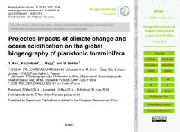
India before emptying into the Bay of Bengal in Bangladesh (Figure 1). The mean annual

106

discharge is approximately 20,000m3/s (Immerzeel, 2008). The climate of the basin is

107

monsoon-driven with an obvious wet season from June to September, which accounts for 60–70%

108

of the annual rainfall.

109

2.2 Data

110

2.2.1 Forcing data sets

111

Due to the lack of adequate in-situ meteorological observations, the WATCH forcing data (WFD)

112

(Weedon et al., 2014) were used as a reference for bias correction and hydrological model

113

calibration (Table 1). This dataset provided a good representation of real meteorological events

114

and climate trends (Weedon et al., 2011). In this study, we used daily rainfall, temperature and

115

potential evapotranspiration (PET) data from 1980 to 2001.

116

The sources of other required non-meteorological variables for implementing the hydrological

117

model are as follows. The 90-m resolution digital elevation model data were acquired from the

118

Shuttle Radar Topography Mission (SRTM) (http://srtm.csi.cgiar.org/). The Leaf Area Index

119

(LAI) and snow cover data from 2000 to 2016 were downloaded from the National Aeronautics

120

and Space Administration (NASA) (https://reverb.echo.nasa.gov/reverb/). For the periods during

121

which LAI and snow data did not cover, average values of LAI and snow were used as model 6


122

input. The biweekly normalized difference vegetation index (NDVI) data from 1982 to 2000

123

with a spatial resolution of 8 km were obtained from the Global Inventory Modeling and

124

Mapping

125

(http://www.glcf.umd.edu/data/gimms/). The soil hydraulic parameters were derived from the

126

soil classification data which were extracted from the global digital soil map with a spatial

127

resolution of 10 km (http://www.fao.org/geonetwork/).

128

2.2.2 Hydrological data

129

The streamflow observations during 1980-2001 for hydrological model calibration were obtained

130

at two hydrological stations, i.e., the Nuxia station located in upstream China (Gao et al. (2008))

131

and the Bahadurabad station located in downstream Bangladesh; see Figure 1 for their

132

geographical locations.

133

2.2.3 RCM data

134

The simulations of daily precipitation and temperature during the historical period of 1980-2001

135

and the projections under two examined emissions scenarios (RCP4.5 and RCP8.5) during the

136

future period of 2020-2035 from the CORDEX experiment for the East Asia domain (which

137

covers the whole YBR Basin) were downloaded from http://www.cordex.org/. The CORDEX

138

program, which was coordinated by the World Climate Research Program, provides a unique

139

opportunity for generating high-resolution regional climate projections and for assessing the

140

impacts of future climate change at regional scales (Piani et al., 2009). As shown in Table 1,

141

climate data from 5 CORDEX models were chosen. These models include HadGEM3-RA

142

(denoted by RCM1), RegCM4 (RCM2), SNU-MM5 (RCM3), SNU-WRF (RCM4) and

143

YSU-RSM (RCM5). To keep consistent with the WATCH forcing data, climate model

144

integrations were interpolated to the grid of the WFD using the bilinear interpolation method.

Studies-Advanced

Very

High

Resolution

7

Radiometer

(GIMMS-AVHRR)


145

The adopted hydrological model, as will be introduced later, also requires PET as a forcing

146

variable. We used the method proposed by Leander and Buishand (2007) and S. C. van Pelt

147

(2009) to calculate PET with daily temperature T as follows: PET = [1 + α0 (T - T0 )] PET0

(1)

148

where T0 is the observed mean temperature (◦C) and PET0 is the observed mean PET0

149

(mm/day) during the historical period. Daily PET0 data were acquired directly from the WFD

150

dataset and were used to compute PET0 . The proportionality constant α0 was determined for

151

each calendar month by regressing the observed PET at each grid cell onto the observed daily

152

temperature.

153

2.3 Methodology

154

2.3.1 Hydrological model: THREW

155

We adopted the Tsinghua Representative Elementary Watershed (THREW) model (Tian, 2006;

156

Tian et al., 2006) to simulate streamflow of the YBR Basin. The model consists of a set of

157

balance equations for mass, momentum, energy and entropy, including associated constitutive

158

relationships for various exchange fluxes, at the scale of a well-defined spatial domain. Details of

159

the model can be found in Tian et al. (2006). The THREW model has been successfully applied

160

to quite a few watersheds across China and United States (Li et al., 2012; Mou et al., 2008; Sun

161

et al., 2014; Tian et al., 2006; Tian et al., 2012; Xu et al., 2015; Yang et al., 2014). For the

162

simulation of snow and glacier melting processes which is important for the YBR Basin, we

163

modify the original THREW model by incorporating the temperature-index method introduced

164

in Hock (2003). The index-temperature method has been shown to exhibit an overall good

165

performance in mountain areas in China (He et al., 2015).

8


166

2.3.2 Bias correction methods

167

Quantile mapping (QM) with reference observations has been routinely applied to correct biases

168

in RCM simulations (Maraun, 2013). Using WFD as reference observations and following the

169

principle of QM, first we estimated cumulative distribution functions (CDFs) for the observed

170

and native RCM-simulated time series of daily precipitation or temperature during the

171

historical/calibration period (which is 1980-2001 in this study); then for a given RCM-simulated

172

data value from an application period (which may be historical 1980-2001 period or future

173

2020-2035 period), we evaluated the CDF of the native RCM simulations at the given data value,

174

followed by evaluation of the inverse of the CDF of the observations at the thus obtained CDF

175

value; the resulting value is the bias-corrected simulation (see Figure 2 for an schematic

176

illustration of this procedure).

177

Independent bias correction for multiple meteorological variables can produce non-physical

178

corrections. To alleviate the deficits of independent bias correction, Li et al. (2014) introduced a

179

joint bias correction (JBC) method, which takes the interactions between precipitation and

180

temperature into account. This approach is based on a general bivariate distribution of P-T and

181

essentially can be seen as a bivariate extension of the commonly used univariate QM method.

182

Depending on the sequence of correction, there are two versions of JBC including JBCp, which

183

corrects precipitation first and then temperature, and JBCt, which corrects temperature first and

184

then precipitation. For more details of the QM and JBC methods, readers can refer to Wlicke et

185

al. (2013) and Li et al. (2014), respectively.

186

2.3.3 Bayesian model averaging method

187

Bayesian model averaging (BMA) is a statistical technique designed to infer a prediction by

188

weighted averaging predictions from different models/simulations. We refer readers to Dong et

9


189

al. (2013), which have presented a nice description of the basic principle of this method and the

190

Expectation-Maximization (EM) algorithm for optimally searching the BMA weights. Several

191

studies have applied BMA to RCMs or GCMs simulations to assess climate change impacts on

192

hydrology with meaningful results (Bhat et al., 2011; Duan et al., 2007; Wang and Robertson,

193

2011; Yang et al., 2011).

194

3. Results and discussion

195

3.1 Bias correction of meteorological variables during the historical period

196

We applied the three bias correction methods (i.e., QM, JBCp and JBCt) to the CORDEX

197

simulations of daily precipitation and temperature. We found that without bias correction, the

198

native RCM1 and RCM2 simulations (see Table 1 for the full names of different RCMs)

199

overestimate precipitation for all months during the 1980-2001 baseline period (Figure 3a-3b),

200

while native simulations by the other models tend to overestimate precipitation of the dry-season

201

(November to May of next year) and underestimate precipitation of other months. After bias

202

correction, the above mentioned overestimation and underestimation reduces considerably. For

203

temperature, we found that all the examined climate models consistently exhibit cold biases

204

across all the months, and that such biases are largely eliminated after applying bias correction

205

(Figure 4). In general, the three bias correction methods exhibit similar skills in reducing

206

temperature biases (Table 2), with JBCt and QM showing somewhat better performance than

207

JBCp. As expected, PET calculated from bias-corrected temperature simulations was quite close

208

to WFD observations.

209

In summary, we found that almost all the bias correction methods can substantially reduce biases

210

for all the three variables across the months, though with sizeable variations between bias

10


211

correction methods and across variables and seasons, consistent with existing studies on the

212

comparison of different bias correction methods (Maraun, 2013; Prasanna, 2016).

213

3.2 Hydrological model setup and simulation

214

To setup the THREW model, the whole basin was discretized into 237 representative elementary

215

watersheds (REWs). There are in total 16 parameters involved in THREW, as listed in Table 3.

216

The first 6 parameters were determined for each REW a prior from the data described in the

217

section ‘Materials and methodology’. The remaining parameters were subjected to calibration

218

and assumed to be uniform across the 237 REWs. Automatic calibration was implemented by the

219

-NSGAII optimization algorithm developed by Reed et al. (2003). We chose the commonly

220

used Nash Sutcliffe efficiency coefficient (NSE) (Nash and Sutcliffe, 1970) as the single

221

objective function for model calibration.

222

We divided the whole period 1980-2001 into two sub-periods, which were used respectively for

223

model calibration (1980-1990) and validation (1991-2001). Simulated daily streamflow time

224

series at Bahadurabad were compared against the corresponding observations to compute the

225

NSE objective function. To warm up the model, we dropped the first year of the calibration

226

period (i.e., 1980). Observed and simulated daily streamflow of remaining years were used to

227

compute NSE as follows: 2

NSE = 1 -

∑Nn=1 (Qno -Qns )

(2)

2

̅̅̅̅) ∑Nn=1 (Qno -Q o

228

where N denotes the total number of days in the calibration period (which is 1981-1990 as one

229

year is dropped for model warming up); Qno and Qns represent respectively the observed and

230

simulated streamflow of day n; and ̅̅̅̅ Qo is the average of observed streamflow during that period.

231

NSE is automatically optimized by the -NSGAII optimization algorithm. With the calibrated

11


232

model, NSE for the 1991-2001 validation period can be likewise computed so as to assess the

233

calibrated model performance in simulating streamflow that is not seen in the calibration period.

234

Figure 5 shows the observed (black line) and simulated (red line) discharges at Bahadurabad at

235

(a) daily, (b) monthly, and (c-d) seasonal time scales for both the calibration and validation

236

periods. It can be seen that the THREW model performs well in the YBR Basin at all time scales.

237

During the calibration period the daily and monthly NSE values are 0.84 and 0.92, respectively,

238

and during the validation period the daily and monthly NSE values are 0.78 and 0.84,

239

respectively. We also compared the observed and simulated monthly discharges at the Nuxia

240

station, which is not involved in model calibration. The monthly NSE values of calibration and

241

validation periods were 0.66 and 0.73, respectively. In summary, these results suggest that the

242

THREW model does a good job in simulating the hydrological processes in the YBR Basin

243

during this historical period. We assume that the calibrated THREW model is applicable to the

244

future period. This assumption is necessary in this study and has been widely adopted in previous

245

climate impacts studies.

246

Figure 6 compares the seasonal streamflow simulated by the THREW model with observed

247

streamflow data at Bahadurabad. It is observed that the streamflow generated by native RCM

248

simulations tends to either over- or underestimate the observations, and that all the adopted bias

249

correction methods can alleviate, to varying degrees, these biases. We found that in general bias

250

correction is more effective in improving the simulation of dry season streamflow (from

251

November to April in the next year) than that of wet season (May to October). Table 4 shows the

252

annual mean observed streamflow at Bahadurabad as well as the simulated streamflow with the

253

WFD data and with the native and bias-corrected RCM integrations. We can see that at annual

254

scale, streamflow simulated with native RCMs is on average higher (e.g., RCM1, RCM2) or

12


255

lower (e.g., RCM3, RCM4 and RCM5) than the observations; while streamflow simulated with

256

bias-corrected RCMs is much more consistent with the observations.

257

Table 5 presents the NSE values for the daily and monthly streamflow over the calibration and

258

validation periods simulated by the THREW model with the WFD data and with native and

259

bias-corrected RCM simulations at Bahadurabad. We found that QM and JBCp can improve

260

NSE for almost all the RCMs except RCM5, while JBCt can improve NSE for three of the five

261

climate models (RCM1, RCM3, and RCM4). We also found that none of the 3 bias correction

262

methods is compelling better than others, suggesting the necessity of combining different

263

streamflow simulations generated with different bias-corrected climate simulations. Moreover, it

264

is seen that most of the NSEs values are higher than 0.55 with a few exceptions, indicating

265

reasonably well simulations of daily and monthly streamflow for both calibration and validation

266

periods on average across the entire basin, and thus enhancing our confidence in applying the

267

calibrated THREW model and the bias-corrected CORDEX simulations to projecting future

268

hydrological conditions in the YBR Basin.

269

Given the fact that none of the bias correction methods and none of the RCM models are

270

compellingly superior over others, as we have found, we therefore integrate streamflow

271

simulations generated by different bias-corrected climate simulations from different climate

272

models with different bias correction methods in terms of BMA. Our attempt is to take

273

advantages of individual streamflow simulations. Daily streamflow simulations and observations

274

during the THREW model calibration period (1981-1990) were used to calibrate the BMA

275

weights, and those during the validation period are used to evaluate the calibrated BMA weights.

276

In addition to NSE, two other indices were used to measure the closeness between observations

13


277

and simulations. These indices are relative error (RE) and root mean squared error (RMSE), both

278

evaluated at daily scale, as defined in the following:

RE = 1 -

∑Nn=1 Qns

(3)

∑Nn=1 Qno (4)

𝑛 𝑛 2 ∑𝑁 𝑛=1(𝑄𝑜 − 𝑄𝑠 ) RMSE = √ 𝑁

279

where N denotes the total number of days during the considered period; 𝑄𝑜𝑛 and 𝑄𝑠𝑛 represent

280

respectively the observed and simulated streamflow of time n. As seen from Table 6, based on

281

the above indices, after applying BMA we obtain considerably better results than almost all those

282

generated by different bias-corrected climate simulations from different climate models with

283

different bias correction methods. Figure 7 shows the mean prediction (red line) and 90%

284

uncertainty interval of BMA during the historical period at Bahadurabad. The uncertainty

285

interval of BMA can cover almost all observations, which further indicated the sound

286

performance of BMA.

287

3.3 Projections of future meteorological variables

288

Figures 8-9 show changes in seasonal precipitation and temperature during the near future period

289

2020-2035 relative to the historical 1980-2001 period based on bias-corrected RCM simulations

290

under RCP4.5 and RCP8.5 emissions scenarios. It is found that precipitation in wet seasons will

291

increase under both emissions scenarios and in all bias-corrected RCM simulations with one

292

exception of RCM3 under RCP4.5. In contrast, precipitation in dry seasons is projected to

293

consistently decrease in all the studied RCM models. Therefore, the general pattern of “wet

294

getting wetter, dry getting drier” (Chou et al., 2013) associate with climate change exists in YBR

295

as well. Also, as expected, precipitation under RCP8.5 is on average higher than that under

14


296

RCP4.5, especially for RCM3 and RCM4 in the wet season. We also found obvious variations in

297

the projected changes among climate models and bias correction methods. This suggests the

298

importance of exploring multi-models and multi-methods to obtain a more comprehensive

299

picture about the uncertainty of the impacts of climate change on local hydrology. Using BMA

300

weight coefficient calculated in Section 3.2, weighted precipitation in historical period, RCP4.5

301

and RCP8.5 is 1425.3, 1529.8 and 1608.0 mm per year, respectively.

302

We found that temperature is projected to increase by all RCM simulations in both dry seasons

303

and wet seasons (Figure 9). It is surprising to see that there is no significant difference in

304

temperature between RCP8.5 and RCP4.5 scenarios except for RCM3 and RCM4. In fact, this is

305

not inconsistent with the IPCC AR5 (2013), which shows that the projected future global mean

306

temperature does not significantly diverge under different RCP scenarios until 2030 (our future

307

period is 2020-2035). Similar to precipitation, there are obvious variations in the projected

308

changes among different climate models and different bias correction methods. Using BMA

309

weight coefficient calculated in Section 3.2, weighted temperature in historical period, RCP4.5

310

and RCP8.5 is 8.7, 9.8 and 10.0℃, respectively.

311

3.4 Projections of future streamflow and comparison with previous studies

312

Figure 10 shows the mean prediction and 90% uncertainty interval of streamflow simulated by

313

BMA method during (a) RCP4.5, (b) RCP8.5 scenarios at Bahadurabad. Uncertainty interval of

314

RCP4.5 is similar with that of RCP8.5. All the following discussions in this subsection is based

315

on BMA weighted streamflow.

316

For the sake of comparison between Immerzeel et al. (2010), Lutz et al. (2014), Masood et al.

317

(2015) and our results, we also examined an upstream outlet location (the red dot in Figure 1),

15


318

which was studied in the referred studies. To be noted, the observed streamflow data at this

319

upstream outlet are unavailable.

320

Table 7 shows a summary of the referred existing studies about climate impact on future

321

streamflow in the YBR Basin. Immerzeel et al. (2010) developed Snowmelt Streamflow Model

322

for the upper YBR Basin using five GCMs in the A1B scenarios defined in IPCC AR4 during

323

2046-2065 without applying any bias correction methods or BMA method and the streamflow

324

will decrease by 19.6% when compared to the observed period (2000-2007). The SPHY model

325

developed by Lutz et al. (2014) for the upper YBR Basin using four GCMs in the RCP4.5 and

326

RCP8.5 scenarios during 2041-2050 and without applying any bias correction methods or BMA

327

method. The streamflow will increase by 4.5% and 5.2% in the RCP4.5 and RCP8.5 scenarios,

328

respectively when compared with the observed period (1998-2007). Masood et al. (2015) applied

329

H08 Hydrological model the YBR Basin using five GCMs during the near future (2015-2039)

330

and far future (2075-2099) and also applied bias correction method. The streamflow increased by

331

6.7% and 16.2% in the near future and far future, respectively, when compared with the observed

332

data (1980-2001).

333

The comparisons among the streamflow projection of YBR during different periods in different

334

studies are shown in Figure 11. In our study, the projected streamflow is 1466 mm/a during

335

2020-2035 under RCP8.5 at Bahadurabad, which is substantially higher than the findings of

336

Masood et al. (2015) at the same location, which is 1244 mm per year during 2015-2039 under

337

RCP8.5. The projected streamflow is 692 mm per year during 2020-2035 under RCP8.5 at the

338

upper YBR outlet. This result is quite close to the findings of Lutz et al. (2014), which is 727

339

mm per year during 2041-2050 under RCP8.5. To be noted, our study adopted RCMs

340

integrations, BMA method by incorporating different bias correction methods, and a physically

16


341

based hydrological model accounting for snow and glacier melting processes, which could

342

explain the differences from the existing studies.

343

Table 8 shows the relative changes of projected runoff and its driving factors under different

344

emission scenarios compared to the historical period at different locations of the YBR. At the

345

basin-wide scale represented by Bahadurabad station, future streamflow shows an evidently

346

increasing trend under both RCP4.5 and RCP8.5 scenarios. The increasing rate under RCP8.5

347

(12.9%) is not-surprisingly higher than RCP4.5 (6.8%). Also, the trends of streamflow exhibit

348

strong spatial variability along the YBR. Under RCP4.5, upstream locations are more likely to

349

experience an increasing trend at a much less rate. For example, the change rate of streamflow is

350

projected to decrease at 0.4% and 4.1% at the YBR outlet and Nuxia, respectively. Under

351

RCP8.5, however, upstream locations would more likely witness an augmented increasing rate of

352

streamflow change, e.g., 13.1% and 19.9% at the YBR outlet and Nuxia, respectively.

353

4. Conclusions

354

In this study, we conducted a comprehensive evaluation of future streamflow in the YBR Basin.

355

We adopted RCMs integrations, BMA method by incorporating different bias correction

356

methods, and a physically based hydrological model accounting for snow and glacier melting

357

processes to implement the evaluation. The major findings are summarized as follows.

358

(1) The three bias correction methods implemented in this study can all substantially reduce

359

biases in the three variables (precipitation, temperature and potential evapotranspiration).

360

Specifically for precipitation, when native RCMs show overestimations, all bias correction

361

methods perform reasonably well. While, none of them can provide satisfying corrections

362

when native RCMs exhibit strong underestimations. This finding is consistent with existing 17


363

studies (Maraun, 2013; Prasanna, 2016) and requires further in-deep studies. For

364

temperature and potential evapotranspiration, all of the three bias correction methods

365

performed well, especially QM and JBCt.

366

(2) The basin-wide discharge is projected to increase substantially during the future period

367

(2020-2035) under the two examined emissions scenarios of RCP4.5 and RCP8.5. The

368

projected annual mean streamflow at Bahadurabad is 1386.7 mm per year under RCP4.5

369

with an increasing rate of 6.9%, and the number becomes higher as 1466.4 mm per year

370

under RCP8.5 with an increasing rate of 12.9%. Increasing mean annual streamflow

371

indicates more flood events that would occur in this already vulnerable region, which calls

372

for more close collaborations among upstream and downstream riparian countries.

373

(3) Projected streamflow exhibits different spatial patterns under different scenarios in the YBR

374

basin. Under RCP4.5, the annual mean streamflow is projected to change by 6.8%, -0.4%,

375

and -4.1% in the future period (2020-2035) compared to the historical period (1980-2001) at

376

three locations from downstream to upstream along the YBR, i.e., Bahadurabad, the upper

377

YBR outlet, and Nuxia. Therefore, the increasing rate of streamflow exhibits an attenuated

378

trend from downstream to upstream. Under RCP8.5, however, the increasing rate of

379

streamflow (12.9%, 13.1%, and 19.9% at the three locations) exhibits an augmented trend

380

from downstream to upstream. The different trends are likely associated with varying spatial

381

patterns of projected future precipitation, but more detailed investigations are needed.

382

18


383

Acknowledgements

384

This study was financially supported by the National Science Foundation of China (91647205),

385

the Ministry of Science and Technology of P.R. China (2016YFA0601603, 2016YFC0402701),

386

and the foundation of State Key Laboratory of Hydroscience and Engineering of Tsinghua

387

University (2016-KY-03).

388

19


389

References

390 391

Arnell, N. W.: Climate change and global water resources, Global Environ. Change, 9, 31-49, 1999.

392 393

Barnett, T. P., Adam, J. C., and Lettenmaier, D. P.: Potential impacts of a warming climate on water availability in snow-dominated regions, Nature, 438, 303-309, 2005.

394 395 396

Bhat, K. S., Haran, M., Terando, A., and Keller, K.: Climate Projections Using Bayesian Model Averaging and Space–Time Dependence, Journal of Agricultural, Biological, and Environmental Statistics, 16, 606-628, 2011.

397 398

Chou, C., Chiang, J. C. H., Lan, C.-W., Chung, C.-H., Liao, Y.-C., and Lee, C.-J.: Increase in the range between wet and dry season precipitation, Nature Geoscience, 6, 263-267, 2013.

399 400 401

Christensen, J. H., Boberg, F., Christensen, O. B., and LucasPicher, P.: On the need for bias correction of regional climate change projections of temperature and precipitation, 2008, Geophysical Research Letters, L20709, 2008.

402 403

Dong, L., Xiong, L., and Yu, K.-x.: Uncertainty Analysis of Multiple Hydrologic Models Using the Bayesian Model Averaging Method, Journal of Applied Mathematics, 2013, 1-11, 2013.

404 405 406

Dosio, A. and Paruolo, P.: Bias correction of the ENSEMBLES high-resolution climate change projections for use by impact models: Evaluation on the present climate, J. Geophys. Res., 116, 2011.

407 408

Duan, Q., Ajami, N. K., Gao, X., and Sorooshian, S.: Multi-model ensemble hydrologic prediction using Bayesian model averaging, Adv. Water Resour., 30, 1371-1386, 2007.

409 410 411

Gain, A. K., Immerzeel, W. W., Sperna Weiland, F. C., and Bierkens, M. F. P.: Impact of climate change on the stream flow of the lower Brahmaputra: trends in high and low flows based on discharge-weighted ensemble modelling, Hydrol. Earth Syst. Sci., 15, 1537-1545, 2011.

412 413 414

Gao, B., Yang, D., Liu, Z., and Zhu, C.: Application of a Distr ibuted Hydrological Model for the Yar lung Zangbo River and Analysis of the River Runoff, Journal of China Hydrology, 28, 40-44, 2008.

415 416

Goswami, D. C.: Brahmaputra River, Assam, India: Physiography, basin denudation, and channel aggradation, Water Resour. Res., 7, 959-978, 1985.

417 418 419

He, Z. H., Tian, F. Q., Gupta, H. V., Hu, H. C., and Hu, H. P.: Diagnostic calibration of a hydrological model in a mountain area by hydrograph partitioning, Hydrol. Earth Syst. Sci., 19, 1807-1826, 2015.

420 421

Hessami, M., Gachon, P., Ouarda, T. B. M. J., and St-Hilaire, A.: Automated regression-based statistical downscaling tool, Environmental Modelling & Software, 23, 813-834, 2008. 20


422 423

Hewitson, B. C. and Crane, R. G.: Climate downscaling: techniques and application, Clim. Res., 7, 85-95, 1996.

424

Hock, R.: Temperature index melt modelling in mountain areas, J. Hydrol., 282, 104-115, 2003.

425 426

Immerzeel, W. W.: Historical trends and future predictions of climate variability in the Brahmaputra basin, Int. J. Climatol., 28, 243-254, 2008.

427 428

Immerzeel, W. W., Van Beek, L. P., and Bierkens, M. F.: Climate change will affect the Asian water towers, Science, 328, 1382-1385, 2010.

429 430

Ines, A. V. M. and Hansen, J. W.: Bias correction of daily GCM rainfall for crop simulation studies, Agric. For. Meteorol., 138, 44-53, 2006.

431 432

Johnson, F. and Sharma, A.: A nesting model for bias correction of variability at multiple time scales in general circulation model precipitation simulations, Water Resour. Res., 48, 2012.

433 434

Leander, R. and Buishand, T. A.: Resampling of regional climate model output for the simulation of extreme river flows, J. Hydrol., 332, 487-496, 2007.

435 436 437

Li, C., Sinha, E., Horton, D. E., Diffenbaugh, N. S., and Michalak, A. M.: Joint bias correction of temperature and precipitation in climate model simulations, J. Geophys. Res. Atmos., 119, 153-162, 2014.

438 439 440

Li, H., Sheffield, J., and Wood, E. F.: Bias correction of monthly precipitation and temperature fields from Intergovernmental Panel on Climate Change AR4 models using equidistant quantile matching, J. Geophys. Res., 115, 2010.

441 442 443

Li, H., Sivapalan, M., and Tian, F.: Comparative diagnostic analysis of runoff generation processes in Oklahoma DMIP2 basins: The Blue River and the Illinois River, J. Hydrol., 418-419, 90-109, 2012.

444 445 446

Lutz, A. F., Immerzeel, W. W., Shrestha, A. B., and Bierkens, M. F. P.: Consistent increase in High Asia's runoff due to increasing glacier melt and precipitation, Nature Climate Change, 4, 587-592, 2014.

447 448

Maraun, D.: Bias Correction, Quantile Mapping, and Downscaling: Revisiting the Inflation Issue, J. Clim., 26, 2137-2143, 2013.

449 450 451

Masood, M., Yeh, P. J. F., Hanasaki, N., and Takeuchi, K.: Model study of the impacts of future climate change on the hydrology of Ganges–Brahmaputra–Meghna basin, Hydrol. Earth Syst. Sci., 19, 747-770, 2015.

452 453 454

Mou, L., Tian, F., Hu, H., and Sivapalan, M.: Extension of the Representative ElementaryWatershed approach for cold regions: constitutive relationships and an application, Hydrol. Earth Syst. Sci., 12, 565, 2008.

21


455 456

Nash, J. E. and Sutcliffe, J. V.: River flow forecasting through conceptual models Part I—A discussion of principles, J. Hydrol., 10, 282-290, 1970.

457 458 459

Olsson, T., Jakkila, J., Veijalainen, N., Backman, L., Kaurola, J., and Vehviläinen, B.: Impacts of climate change on temperature, precipitation and hydrology in Finland – studies using bias corrected Regional Climate Model data, Hydrol. Earth Syst. Sci., 19, 3217-3238, 2015.

460 461

Piani, C., Haerter, J. O., and Coppola, E.: Statistical bias correction for daily precipitation in regional climate models over Europe, Theor. Appl. Climatol., 99, 187-192, 2009.

462 463 464

Piani, C., Weedon, G. P., Best, M., Gomes, S. M., Viterbo, P., Hagemann, S., and Haerter, J. O.: Statistical bias correction of global simulated daily precipitation and temperature for the application of hydrological models, J. Hydrol., 395, 199-215, 2010.

465 466 467

Prasanna, V.: Statistical bias correction method applied on CMIP5 datasets over the Indian region during the summer monsoon season for climate change applications, Theor. Appl. Climatol., doi: 10.1007/s00704-016-1974-8, 2016. 2016.

468 469

Rauscher, S. A., Coppola, E., Piani, C., and Giorgi, F.: Resolution effects on regional climate model simulations of seasonal precipitation over Europe, Clim. Dyn., 35, 685-711, 2010.

470 471 472

Reed, P., Minsker, B. S., and Goldberg, D. E.: Simplifying multiobjective optimization: An automated design methodology for the nondominated sorted genetic algorithm-II, Water Resour. Res., 39, 2003.

473 474 475

S. C. van Pelt, P. K., H.W. ter Maat, B. J. J. M. van den Hurk, and A. H.Weerts: Discharge simulations performed with a hydrological model using bias corrected regional climate model input, Hydrol. Earth Syst. Sci., 13, 2387-2397, 2009.

476 477 478

Sun, Y., Tian, F., Yang, L., and Hu, H.: Exploring the spatial variability of contributions from climate variation and change in catchment properties to streamflow decrease in a mesoscale basin by three different methods, J. Hydrol., 508, 170-180, 2014.

479 480 481

Thrasher, B., Maurer, E. P., McKellar, C., and Duffy, P. B.: Technical Note: Bias correcting climate model simulated daily temperature extremes with quantile mapping, Hydrol. Earth Syst. Sci., 16, 3309-3314, 2012.

482 483

Tian, F.: Study on Thermodynamic Watershed Hydrological Model (THModel), Ph.D. Thesis, 2006. Department of Hydraulic Engineering, Tsinghua University, Beijing, China, 168 pp., 2006.

484 485 486

Tian, F., Hu, H., Lei, Z., and Sivapalan, M.: Extension of the Representative ElementaryWatershed approach for cold regions via explicit treatment of energy related processes, Hydrol. Earth Syst. Sci., 10, 619-644, 2006.

487 488

Tian, F., Li, H., and Sivapalan, M.: Model diagnostic analysis of seasonal switching of runoff generation mechanisms in the Blue River basin, Oklahoma, J. Hydrol., 418-419, 136-149, 2012.

22


489 490

Tong, K., Su, F., Yang, D., Zhang, L., and Hao, Z.: Tibetan Plateau precipitation as depicted by gauge observations, reanalyses and satellite retrievals, Int. J. Climatol., 34, 265-285, 2014.

491 492

Wang, Q. J. and Robertson, D. E.: Multisite probabilistic forecasting of seasonal flows for streams with zero value occurrences, Water Resour. Res., 47, 2011.

493 494 495

Weedon, G. P., Balsamo, G., Bellouin, N., Gomes, S., Best, M. J., and Viterbo, P.: The WFDEI meteorological forcing data set: WATCH Forcing Data methodology applied to ERA-Interim reanalysis data, Water Resour. Res., 50, 7505-7514, 2014.

496 497 498 499

Weedon, G. P., Gomes, S., Viterbo, P., Shuttleworth, W. J., Blyth, E., Österle, H., Adam, J. C., Bellouin, N., Boucher, O., and Best, M.: Creation of the WATCH Forcing Data and Its Use to Assess Global and Regional Reference Crop Evaporation over Land during the Twentieth Century, J. Hydrometeorol., 12, 823-848, 2011.

500 501

Wlicke, R. A. I., Mendlik, T., and Gobiet, A.: Multi-variable error correction of regional climate models, Climate Change, 120, 871-887, 2013.

502 503 504

Xu, R., Tian, F., Yang, L., Hu, H., Lu, H., and Hou, A.: Ground validation of GPM IMERG and TRMM 3B42V7 rainfall products over southern Tibetan Plateau based on a high-density rain gauge network, J. Geophys. Res. Atmos., 122, 910-924, 2017.

505 506 507

Xu, R., Tie, Q., Dai, C., Hu, H., and Tian, F.: Study on hydrological process in upper basin of Brahmaputra River from Nuxia Hydrological Station and its response to climate change (in Chinese), Journal of Hohai University (Natural Sciences), 43, 288-293, 2015.

508 509

Yang, H., Wang, B., and Wang, B.: Reducing biases in regional climate downscaling by applying Bayesian model averaging on large-scale forcing, Clim. Dyn., 39, 2523-2532, 2011.

510 511

Yang, L., Tian, F., Sun, Y., Yuan, X., and Hu, H.: Attribution of hydrologic forecast uncertainty within scalable forecast windows, Hydrol. Earth Syst. Sci., 18, 775-786, 2014.

512 513

23


514

List of Tables

515

Table 1. Description of the WATCH forcing data and 5 RCM datasets. ..................................... 25

516

Table 2. Annual mean values of basin-wide precipitation (ppt), temperature (tmp) and potential

517

evapotranspiration (pet) calculated from WFD and native/corrected RCMs datasets. ................. 26

518

Table 3. Principal parameters of THREW model. ........................................................................ 27

519

Table 4. Annual mean observed discharge and simulated discharge forced by WFD and

520

native/corrected RCMs datasets at the Bahadurabad station. ....................................................... 28

521

Table 5. Nash-Sutcliffe efficiency coefficient (NSE) of streamflow simulation forced by WFD

522

and native/corrected RCMs datasets at daily and monthly time scales (denoted as day and mon in

523

the table)........................................................................................................................................ 29

524

Table 6. Evaluation merits of streamflow simulations for individual RCM and BMA scenarios. 30

525

Table 7. Summary of existing studies on projected streamflow under climate change in the YBR

526

Basin. ............................................................................................................................................ 31

527

Table 8. Means of precipitation / temperature / runoff in the future period (2020-2035) and their

528

relative changes compared to the historical period (1980-2001) under different scenarios in the

529

YRB. ............................................................................................................................................. 32

530

24


Table 1. Description of the WATCH forcing data and 5 RCM datasets.

531 Type

Dataset

Spatial resolution

Temporal resolution

Period

Description

Observation data

WATCH Forcing Data

0.5°

Daily

1980-2001

Rainfall, air temperature, potential evapotranspiration

0.44°

Daily

1980-2001

Rainfall, air temperature, surface pressure, specific humidity

(WFD) RCM data

HadGEM3-RA (RCM1)

2020-2035 (RCP4.5, RCP8.5)

RegCM (RCM2) SNU-MM5 (RCM3) SNU-WRF (RCM4) YSU-RSM (RCM5)

532 533

25


534

Table 2. Annual mean values of basin-wide precipitation (ppt), temperature (tmp) and potential

535

evapotranspiration (pet) calculated from WFD and native/corrected RCMs datasets. native

JBCp

JBCt

QM

ppt

WFD

1310

mm /yr

RCM1

2025

1296

1283

1296

RCM2

1834

1312

1299

1312

RCM3

1101

1584

1726

1584

RCM4

1242

1523

1617

1523

RCM5

1381

1325

1338

1325

tmp

WFD

8.77

℃

RCM1

5.80

8.85

8.77

8.77

RCM2

4.48

8.69

8.77

8.77

RCM3

4.99

8.23

8.77

8.77

RCM4

3.77

8.57

8.77

8.77

RCM5

0.36

8.38

8.77

8.77

pet

WFD

532

mm /yr

RCM1

448

525

542

542

RCM2

430

528

542

542

RCM3

474

526

553

553

RCM4

479

540

543

543

RCM5

478

513

532

532

536 537

26


Table 3. Principal parameters of THREW model.

538 Symbol

Unit

Physical meaning

Range

Ks u

m/s

-

Ks s

m/s

-

6.25e-6

εu

-

-

0.47

εs ψα

m

-

0.28 0.25

μ

-

Saturated hydraulic conductivity for u-zone which is different for each REW. The value showing here is the averaged value over the whole catchment Similar to Ksu, saturated hydraulic conductivity for s-zone Soil porosity value of u-zone which is different for each REW. The value showing here is averaged over the whole catchment Similar toεu, soil porosity of s-zone Air entry value which is different for each REW. The value showing here is averaged over the whole catchment Soil pore size distribution index in

Calibrated value 6.25e-6

-

0.20

0.005-1 0.005-1

0.03 0.006

0.1-1

0.5

1-30

5.0

0.1-1 0.1-5

0.5 1.5

0.1-20

0.7

0.1-5

0.7

0-15 0-15

6.0 4.8

f e   EFL

u s

K (1  s u ) y u

( S u )2 d  u  a



, where

fe

is the

exfiltration capacity from u-zone, s is the saturation degree of u-zone, y u is the soil depth of u-zone, d is u

the diffusion index nt nr

-

B

-

KKA

-

(d  1  1/  ) .

The value showing

here is the averaged value over the whole catchment Manning roughness coefficient for hillslope Similar to nr , Manning roughness coefficient for channel Shape coefficient to calculate the saturation excess streamflow area Coefficient to calculate subsurface flow in S Rg  KKD  S  K  ( y S S

Z

)

KKA

, When S is the topographic

s

αIFL

-

αEFL

-

αETL

-

DDFg DDFs

mm℃day-1 mm℃day-1

KKD

slope, y is the depth of s-zone, Z is the total soil depth See describe for KKA Spatial heterogeneous coefficient for infiltration capacity Spatial heterogeneous coefficient for exfiltration capacity Spatial heterogeneous coefficient for evapotranspiration capacity Degree day factor glacier Degree day factor snow

539 540

27


541

Table 4. Annual mean observed discharge and simulated discharge forced by WFD and native/corrected

542

RCMs datasets at the Bahadurabad station. Discharge

Calibration period

Validation period

104m3/s

native

obs

2.23

2.29

WFD

2.08

2.09

RCM1

3.12

2.01

2.07

1.97

RCM2

2.73

2.03

2.05

RCM3

1.80

2.34

RCM4

1.88

RCM5

2.02

QM

JBCp

JBCt

QM

JBCp

JBCt

3.23

2.11

2.16

2.07

2.00

2.85

2.12

2.15

2.09

2.31

2.55

1.84

2.37

2.33

2.61

2.24

2.25

2.41

1.92

2.27

2.28

2.45

1.87

1.89

1.90

2.24

2.08

2.10

2.13

543 544 545

28

native


546

Table 5. Nash-Sutcliffe efficiency coefficient (NSE) of streamflow simulation forced by WFD and native/corrected RCMs datasets at daily and

547

monthly time scales (denoted as day and mon in the table). NSE

RCM1

RCM2

RCM3

RCM4

RCM5

calibration

validation

calibration

validation

calibration

validation

calibration

validation

calibration

validation

day

mon

day

mon

day

mon

day

mon

day

mon

day

mon

day

mon

day

mon

day

mon

day

mon

WFD

0.84

0.92

0.78

0.84

RCM

-0.1

0.10

-0.0

0.17

0.46

0.61

0.39

0.51

0.52

0.64

0.40

0.53

0.56

0.70

0.56

0.67

0.56

0.69

0.54

0.70

RCM_QM

0.53

0.66

0.56

0.66

0.51

0.63

0.47

0.57

0.57

0.69

0.44

0.58

0.56

0.72

0.58

0.70

0.41

0.51

0.51

0.63

RCM_JBCp

0.56

0.69

0.58

0.69

0.53

0.66

0.49

0.60

0.58

0.71

0.46

0.60

0.57

0.72

0.59

0.70

0.42

0.52

0.51

0.63

RCM_JBCt

0.44

0.56

0.50

0.60

0.39

0.50

0.35

0.43

0.59

0.72

0.51

0.65

0.60

0.76

0.64

0.75

0.49

0.59

0.56

0.69

548

29


549

Table 6. Evaluation merits of streamflow simulations for individual RCM and BMA scenarios. Scenarios

QM

JBCp

JBCt

BMA

Calibration

Validation

NSE

RE (%)

RMSE (m3/s)

NSE

RE (%)

RMSE (m3/s)

RCM1

0.53

9.9

12070.7

0.56

7.8

12519.3

RCM2

0.51

9.0

12312.7

0.47

7.1

13701.0

RCM3

0.57

-4.9

11573.7

0.44

-3.8

14158.6

RCM4

0.56

-0.5

11633.8

0.58

0.5

12174.1

RCM5

0.41

16.3

13487.3

0.51

8.9

13269.3

RCM1

0.56

7.2

11703.5

0.58

5.4

12244.0

RCM2

0.53

8.1

12061.4

0.49

6.0

13424.4

RCM3

0.58

-3.4

11369.7

0.46

-1.9

13898.5

RCM4

0.57

-0.9

11568.2

0.59

0.3

12134.9

RCM5

0.42

15.4

13427.7

0.50

8.1

13264.3

RCM1

0.44

11.9

13111.4

0.50

9.4

13374.6

RCM2

0.39

10.5

13732.9

0.35

8.5

15243.1

RCM3

0.59

-15.0

11204.6

0.51

-14.1

13165.9

RCM4

0.60

-7.9

11161.9

0.64

-7.4

11347.8

RCM5

0.49

15.0

12613.0

0.62

6.9

12564.8

0.64

6.9

10524.2

0.61

4.8

11745.9

30


Table 7. Summary of existing studies on projected streamflow under climate change in the YBR Basin.

550 Hydrological model

Snowmelt Runoff Model

Study Area, Calibration Hydrological Station upper YBR Basin, no calibration station

GCMs/RCMs

Scenarios

GCMs (CCMA-CGCM3, GFDL-CM2,MPIM-ECHAM5,NIES-MIROC3, UKMO-HADGEM1)

Spatial Processes in Hydrology (SPHY) model

upper YBR Basin, no calibration station

GCMs (RCP4.5:GISS-E2-R, IPSL-CM5A-LR, CCSM4, CanESM2; RCP8.5: GFDL-ESM2G, IPSL-CM5A-LR, CSIRO-Mk3-6-0, CanESM2)

H08 Hydrological model

YBR Basin, Bahadurabad

GCMs (MRI-AGCM3.2S, MIROC5, MIROC-ESM, MRI-CGCM3, HadGEM2-ES)

Tsinghua Representative Elementary Watershed (THREW) model

YBR Basin, Bahadurabad

RCMs(HadGEM3-RA, RegCM, SNU-MM5, SNU-WRF, YSU-RSM)

551 552

31

Obs (2000-2007) A1B (2046-2065) Obs (1998-2007) RCP4.5 (2041-2050) RCP8.5 (2041-2050) Obs (1980-2001) Near-future (2015-2039) Far-future (2075-2099) Obs (1980-2001) RCP4.5 (2006-2035) RCP8.5 (2006-2035)

Bias Correction

Bayesian Model Averaging

Streamflow Change Results

Reference

No

No

-19.6%

Immerzeel et al. (2010)

No

No

4.5%(RCP4.5) 5.2%(RCP8.5)

Lutz et al. (2014)

Yes

No

6.7%(near-future) 16.2%(far-future) RCP8.5

Masood et al. (2015)

Yes

Yes

6.8%(RCP4.5) 12.9%(RCP8.5)

This study


553

Table 8. Means of precipitation / temperature / runoff in the future period (2020-2035) and their relative changes compared to the historical period

554

(1980-2001) under different scenarios in the YRB.

555 556 557 558

P

RP

T

RT

R

RR

(mm/a)

(%)

(℃)

(℃)

(mm/a)

(%)

His-B

1425.3

-

8.7

-

1298.4

fs4.5-B

1529.8

7.3%

9.8

1.1

fs8.5-B

1608.0

12.8%

10.0

1.3

His-O

668.9

-

1.0

fs4.5-O

639.9

-4.4%

fs8.5-O

748.3

11.9%

His-N

631.6

fs4.5-N

595.8

fs8.5-N

712.0

rR

rG

rS

-

87.0%

3.2%

97%

1386.7

6.8%

86.5%

3.3%

10.2%

1466.4

12.9%

86.9%

3.2%

10.0%

-

611.6

-

68.9%

9.0%

22.1%

2.2

1.3

609.3

-0.4%

64.4%

9.9%

25.7%

2.6

1.6

691.9

13.1%

67.4%

9.0%

23.6%

-

-0.1

-

485.8

-

74.4%

5.3%

20.3%

-5.7%

1.2

1.3

465.8

-4.1%

69.3%

6.1%

24.6%

12.7%

1.6

1.7

582.5

19.9%

74.8%

5.0%

20.3%

Note: P denotes precipitation, T denotes temperature, R denotes runoff; RP, RT, RR denote relative changes of P, T and R compared to the historical period, respectively; rR, rG, rS denotes the ratio of rainfall, glacier melting, and snow melting induced runoff in the total runoff, respectively; -B denotes Bahadurabad, -O denotes he upper YBR basin outlet, and -N denotes Nuxia.

32


559

List of Figures

560

Figure 1. Study area, river network and location of hydrological stations (Nuxia in the upstream

561

basin, Bahadurabad in the downstream basin). ............................................................................. 34

562

Figure 2. Schematic illustration of quantile mapping bias correction method applied in the paper

563

(Wlicke et al., 2013)...................................................................................................................... 35

564

Figure 3. Seasonal cycles of precipitation from WFD and native/corrected RCMs during the

565

historical period (1980-2001). (a) for RCM1, (b) for RCM2, (c) for RCM3, (d) for RCM4, (e) for

566

RCM5............................................................................................................................................ 36

567

Figure 4. Seasonal cycles of temperature from WFD and native/corrected RCMs during the

568

historical period (1980-2001). (a) for RCM1, (b) for RCM2, (c) for RCM3, (d) for RCM4, (e) for

569

RCM5............................................................................................................................................ 37

570

Figure 5. The simulated (red line) and observed (black line) discharge at Bahadurabad at the (a)

571

daily scale, (b) monthly scale........................................................................................................ 38

572

Figure 6. Seasonal cycles of observed streamflow and simulated streamflow forced by WFD and

573

native/corrected RCMs during the calibration period (left column) and validation period (right

574

column) at Bahadurabad. .............................................................................................................. 39

575

Figure 7. The mean values and 90% uncertainty interval of streamflow simulated by the BMA

576

method during the historical period. ............................................................................................. 40

577

Figure 8. Change of basin-wide precipitation in the future period projected by corrected RCMs

578

under RCP4.5 (left column) and RCP8.5 (right column) scenarios compared to the historical

579

period. ........................................................................................................................................... 41

580

Figure 9. Change of basin-wide temperature in the future period projected by corrected RCMs

581

under RCP4.5 (left column) and RCP8.5 (right column) scenarios compared to the historical

582

period. ........................................................................................................................................... 42

583

Figure 10. The mean values and 90% uncertainty interval of streamflow simulated by the BMA

584

method during the future period under (a) RCP4.5, (b) RCP8.5 scenarios at Bahadurabad. ....... 43

585

Figure 11. Streamflow projections from the existing studies during different periods at different

586

locations (B denotes Bahadurabad in the downstream, O denotes the upper YBR basin outlet, see

587

Figure 1 for the location). ............................................................................................................. 44

588 33


589 590

Figure 1. Study area, river network and location of hydrological stations (Nuxia in the upstream basin,

591

Bahadurabad in the downstream basin).

34


592 593

Figure 2. Schematic illustration of quantile mapping bias correction method applied in the paper (Wlicke

594

et al., 2013).

595

35


596 597

Figure 3. Seasonal cycles of precipitation from WFD and native/corrected RCMs during the historical

598

period (1980-2001). (a) for RCM1, (b) for RCM2, (c) for RCM3, (d) for RCM4, (e) for RCM5.

599

36


600 601

Figure 4. Seasonal cycles of temperature from WFD and native/corrected RCMs during the historical

602

period (1980-2001). (a) for RCM1, (b) for RCM2, (c) for RCM3, (d) for RCM4, (e) for RCM5.

603

37


604 605

Figure 5. The simulated (red line) and observed (black line) discharge at Bahadurabad at the (a) daily

606

scale, (b) monthly scale.

607

38


608 609

Figure 6. Seasonal cycles of observed streamflow and simulated streamflow forced by WFD and

610

native/corrected RCMs during the calibration period (left column) and validation period (right column) at

611

Bahadurabad.

39


612 613

Figure 7. The mean values and 90% uncertainty interval of streamflow simulated by the BMA method

614

during the historical period.

615

40


616 617

Figure 8. Change of basin-wide precipitation in the future period projected by corrected RCMs under

618

RCP4.5 (left column) and RCP8.5 (right column) scenarios compared to the historical period.

619 41


620 621

Figure 9. Change of basin-wide temperature in the future period projected by corrected RCMs under

622

RCP4.5 (left column) and RCP8.5 (right column) scenarios compared to the historical period.

623 42


624 625

Figure 10. The mean values and 90% uncertainty interval of streamflow simulated by the BMA method

626

during the future period under (a) RCP4.5, (b) RCP8.5 scenarios at Bahadurabad.

627

43


628 629

Figure 11. Streamflow projections from the existing studies during different periods at different locations (B denotes Bahadurabad in the

630

downstream, O denotes the upper YBR basin outlet, see Figure 1 for the location).

44

Projected Climate Change Impacts on Future Streamflow of the

Projected Climate Change Impacts on Future Streamflow of the

Suggest Documents

Modelling the impacts of projected future climate change on water ...

Quantifying climate change impacts on streamflow ...

Modelling the impacts of projected future climate

Projected climate change impacts on spatial ...

Addressing Climate Change Impacts on Streamflow in the ... - MDPI

Projected climate change impacts on the ... - Wiley Online Library

Modeling Potential Impacts of Climate Change on Streamflow ... - MDPI

Comparing impacts of climate change on streamflow in four large ...

Projected Economic Impacts of Climate Change on Irish Agriculture

Projected impacts of climate change on farmers ... - BioMedSearch

Projected impacts of climate change on farmers ... - Semantic Scholar

Potential impacts of projected climate change on safe carrying ...

Projected impacts of climate change on habitat availability for ... - PLOS

Observed and projected impacts of climate change on ...

Projected impacts of climate change on salmon habitat restoration

Projected Impacts of Climate Change on Forests ... - HimalDoc - ICIMOD

Impacts of Projected Climate Change over the Lake Champlain Basin ...

Impacts of climate change on the future of biodiversity

Assessing the Impacts of Future Climate Change on Protected Area ...

Climate Change Impacts on the Future Distribution of Date ... - PLOS

Projected impacts of climate change and ocean ... - Biogeosciences

Projected impacts of climate change and ocean acidification - CiteSeerX

Review of climate change impacts on future carbon stores and ...

Perceptions of Present and Future Climate Change Impacts on ... - MDPI