2- Hong Kong Baptist University, Kowloon - Hong Kong. 3- University of ..... "Ar" u 1:2. "Br" u 1:2. "Cr" u 1:2. "Dr" u 1:2. "Er" u 1:2. "Fr" u 1:2. "Gr" u 1:2. "Hr" u 1:2.
ESANN'2009 proceedings, European Symposium on Artificial Neural Networks - Advances in Computational Intelligence and Learning. Bruges (Belgium), 22-24 April 2009, d-side publi., ISBN 2-930307-09-9.
Projection of undirected and non-positional graphs using Self Organizing Maps Markus Hagenbuchner1 and ShuJia Zhang1 and Ah Chung Tsoi 2 and Alessandro Sperduti3
∗
1- University of Wollongong, Wollongong, NSW 2522 - Australia 2- Hong Kong Baptist University, Kowloon - Hong Kong 3- University of Padova, 35121 Padova, Padova - Italy Abstract. Kohonen’s Self-Organizing Map is a popular method which allows the projection of high dimensional data onto a low dimensional display space. Models of Self-Organizing Maps for the treatment of graphs have also been defined and studied. This paper proposes an extension to the GraphSOM model which substantially improves the stability of the model, and, as a side effect, allows for an acceleration of training. The proposed extension is based on a soft encoding of the information needed to represent the vertices of an input graph. Experimental results demonstrate the advantages of the proposed extension.
1 Introduction Kohonen’s Self-Organizing Map (SOM) is an unsupervised machine learning model which is popularly applied to tasks requiring the clustering of high dimensional vectorial data into groups, or the projection of high dimensional data vectors onto lower dimension display space[1]. However, data involved in many real world problems is naturally presented in the form of sequences or graphs. For example, in speech recognition, the data is generally made available as a temporal sequence. Often, the meaning of a given sequence is not known, and hence, unsupervised machine learning methods are needed to group the data together according to some similarity criterion [1]. However, most learning problems are more suitably represented by richer structures such as trees and graphs. For example, data in molecular chemistry are more appropriately represented as a graph where nodes represent the atoms of a molecule, and the links between nodes represent atomic bindings. Recent developments allowed the processing of graph structured data by a SOM such that the projection is made from a domain of graphs to a fixed-dimensional display space [2, 3, 4, 5, 6, 7]. Among these models, SOM for Structured Data (SOM-SD) [2, 4] and Contextual SOM-SD (CSOM-SD) [5] can only deal with directed acyclic graphs. Specifically, SOM-SD is computationally limited to encoding causal relationships between nodes in a tree structure, while CSOM-SD computationally allows the contextual processing of nodes, i.e. is able to “discriminate” in which context a rooted substructure is found, i.e. who are the ancestors and descendants of ancestors of the substructure’s root. The remaining models are able to deal with more generic graphs: the one proposed in [3] is a standard SOM using a specific graph edit distance, the Merge SOM (MSOM) learns recursive dependencies through a fractal encoding [8], and the GraphSOM model proposed in [6], which is able to deal with undirected and ∗ This research has been funded in part by the Australian Research Council in form of a Discovery Project grant DP0774168.
559
ESANN'2009 proceedings, European Symposium on Artificial Neural Networks - Advances in Computational Intelligence and Learning. Bruges (Belgium), 22-24 April 2009, d-side publi., ISBN 2-930307-09-9.
non-positional graphs by representing each graph vertex through the activation pattern generated on the SOM by its neighbours. The purpose of this paper is to propose an enhancement to one of the before mentioned approached (viz the GraphSOM). We point out that the GraphSOM must be trained very carefully as it can become unstable quite quickly. This in turn can slow the training procedure considerably. We propose an extension to the GraphSOM which prevents the unstable nature of the GraphSOM. A side effect of the proposed method is that the training procedure can be optimized very effectively resulting in significantly reduced training times. This paper is organized as follows. Section 2 provides an explanation of the GraphSOM, and introduces extensions which allow for a substantial improvement. Section 3 makes comparisons between the performance of the GraphSOM and that of the proposed extension through a set of experiments. Conclusions are drawn in Section 4.
2 Self-Organizing Maps for Graphs In general, SOMs [1] consist of a collection of neurons which are arranged on a regular q-dimensional grid called a display space or map, where often q=2. An n-dimensional codebook vector m is attached to each neuron; the dimension of the input to a SOM is assumed to be of the same dimension. Training a SOM is performed in two steps: Competitive step: Given the j-th input vector xj ∈ IRn , the best matching codebook is determined, e.g. by using the Euclidean distance measure as follows [1]: r
=
arg min k(xj − mi )T Λk, i
(1)
where the superscript T denotes the transpose of a vector, and, for the traditional SOM algorithm [1], the Λ is a diagonal matrix with all diagonal elements set to 1. Cooperative step: The winning neuron and all its neighbors are updated as follows: ∆mi
= α(t)f (∆ir )(xi − u),
(2)
where α is a learning rate decreasing to 0 with time t, f (·) is³a neighborhood function ´ 2 i −lr k which is often a Gaussian function [1], i.e., f (∆ir ) = exp − kl2σ(t) where σ is , 2 called the neighborhood radius which decreases with time t to a value > 1, lr and li are the coordinates of the winning neuron and the i-th neuron in the lattice respectively. The two steps are executed for each input vector, and for a given number of iterations [1]. When processing graphs, the input vectors x are formed through a concatenation of a numeric data label which may be associated with a given node, and the state information about the node’s offsprings or neighbors. There are two possibilities of interpretation of the term: state. In [2, 5] the state of an offspring or neighbor is said to be the mapping of the offspring or the neighbor, whereas in [6] the state is said to be the activation of the SOM when mapping all the node’s neighbors or offsprings. This paper addresses an enhancement of the GraphSOM approach in [6], and hence the following will focus on the GraphSOM approach.. In [6] the input vector is formed through xj = (uj , Mne[j] ), where uj is a numeric data vector associated with the j-th node, Mne[j] is a |M|-dimenssional vector containing the activation of the map M when presented with all neighbors of node j. An element Mi of the map is zero if none of the neighbors are mapped at the i-th neuron
560
ESANN'2009 proceedings, European Symposium on Artificial Neural Networks - Advances in Computational Intelligence and Learning. Bruges (Belgium), 22-24 April 2009, d-side publi., ISBN 2-930307-09-9.
location, otherwise it is the number of neighbors that were mapped at that location. This approach produces fixed sized input vectors. Note also that the latter approach requires knowledge of the mappings of all of a node’s neighbors. The availability of these mappings cannot be assured when dealing with undirected or cyclic graphs. This is overcome in [6] by utilizing the mappings from a previous time step. The approximation is valid since convergence is guaranteed. It can be observed that the inclusion of state information in the input vector provides a local view of the graph structure. The iterative nature of the training algorithm ensures that local views are propagated, and hence, structural information about the graph is passed on to all reachable nodes. The input vectors x to the GraphSOM contain hybrid information (label and state information). The diagonal matrix Λ is used to control the influence of these components on the mapping. The diagonal elements λ11 · · · λpp are set to µ ∈ (0; 1), all remaining diagonal elements are set to 1 − µ, where p = |u|. The constant µ influences the contribution of the data label, and the state component to the Euclidean distance. A weakness of the GraphSOM is that the Euclidean distance measure in Eq. 1 does not make a distinction as whether any change of a mapping during the update step has been to a nearby location or to a far away location on the map. This defeats the very purpose to achieve topology preserving properties, and can cause alternating states to occur. To counter this behavior it is necessary to either significantly reduce the learning rate (causing long training times), or to use a large value for µ (causing a neglect of structural information). This paper proposes to soft code the mappings of neighbors to account for the probabilities of any changes in the mapping of nodes. In other words, instead of hard coding the mappings of nodes to be either 1 if there is a mapping at a given location, or 0 if there is no mapping at a given location, we propose to code the likelihood of a mapping in a subsequent iteration with a probability value. We note that due to the effects of Eq. 2 it is most likely that the mapping of a node will be unchanged at the next iteration. But since all neurons are updated, and since neurons which are close to a winner neuron (as measured by Euclidean distance) are updated more strongly (controlled by the Gaussian function), and, hence, it is more likely that any change of a mapping will be to a nearby location than to a far away location. These likelihoods are directly influenced by the neighborhood function and its spread. Hence, we propose to incorporate −
kli −lr k2 2σ(t)2
e√
the likelihood of a mapping in subsequent iterations as follows: Mi = , 2πσ(t) where σ(t) decreases with time t towards zero, all other quantities are as defined before. The computation is cumulative for all of Pthe i-th node’s neighbors. Note that the 1 term √2πσ(t) normalizes the states such that i Mi ≈ 1.0. This approach accounts for the fact that during the early stages of the training process it is likely that mappings can change significantly, whereas towards the end of the training process, as σ(t) → 0, the state vectors become more and more similar to the hard coding method. Section 3 will show that this approach improves the stability of the GraphSOM significantly, allowing the setting of large learning rates which reduces the required training time while providing an overall improvement in the clustering performance. For ease of reference, we refer to this approach as the probability mapping GraphSOM (PM-GraphSOM). This approach produces state vector elements which are non-zero, as compared with the GraphSOM where the state vector can be sparse; this creates the opportunity for an
561
ESANN'2009 proceedings, European Symposium on Artificial Neural Networks - Advances in Computational Intelligence and Learning. Bruges (Belgium), 22-24 April 2009, d-side publi., ISBN 2-930307-09-9.
Table 1: A comparison of performances between PM-GraphSOM and the GraphSOM. GraphSOM PM-GraphSOM Classification Performance 79.624% 90.178% Clustering Performance 69.60% 78.04% Training Time 10mins 8mins optimization of the competitive step. Since the Euclidean distance is computed through element-wise computations on two vectors, and since we are only interested in finding the best matching codebook, hence, the computation of the Euclidean distance can be interrupted as soon as the partial sum exceeds a previously found minimum distance. This was found to be very effective in practice reducing the computational demand of the competitive step by as much as 70%.
3 Experiments and Results To illustrate the effect of the proposed approach, the GraphSOM and the PM-GraphSOM are applied to the Policemen benchmark (available from www.artificial-neural.net). The benchmark problem consists of 3750 trees which were extracted from images featuring policemen, houses, and ships. The nodes of the tree correspond to regions of uniform color in the original image, links between the nodes show how the regions are connected in the image. A label is associated with each node indicating the coordinates of the center of gravity of the region. The dataset defines 12 pattern classes. These are used to identify the quality of the clustering, and are not used during training. The clustering performance is a more sophisticated approach to computing the ability of a GraphSOM to suitably group data on the map. It is computed as is shown in [9]. The equations are ommited here due to space restrictions. A variety of maps and training parameters were tried. A typical observation is illustrated in Table 1 which present the results of maps of size 120 × 80 trained using identical training parameters for PM-GraphSOM and GraphSOM. From Table 1 it is observed that the performance improvement is substantial when compared to that of the GraphSOM approach, and that this improvement is achieved at a reduced computational time. In fact, we found that in all experiments conducted, the PM-GraphSOM always outperformed the GraphSOM by a margin. The resulting mappings are shown in Fig. 1. The upper two plots in Fig. 1 show the mapping of (labeled) root nodes, the lower two plots show the mapping of all nodes. From Fig. 1 it can be observed that the performance improvement can be attributed to a better condensation of the pattern classes, and a better utilization of the mapping space which became possible through the probability mappings which are richer in information. We then applied the GraphSOM methods to a practical data mining learning problem involving XML formatted documents from Wikipedia. This is a very recent dataset used as a benchmark problem for clustering algorithms which are defined on graphs (see http://xmlmining.lip6.fr). The dataset consists of 114, 366 documents which are linked through hyperlinks. This is represented as a graph by assigning documents to be nodes in the graph, and the topology of the graph is defined through the hyperlinks between the documents. This produces a directed graph containing 636, 187 links and
562
ESANN'2009 proceedings, European Symposium on Artificial Neural Networks - Advances in Computational Intelligence and Learning. Bruges (Belgium), 22-24 April 2009, d-side publi., ISBN 2-930307-09-9.
80
80 "xr" u 1:2 "yr" u 1:2 "Ar" u 1:2 "Br" u 1:2 "Cr" u 1:2 "Dr" u 1:2 "Er" u 1:2 "Fr" u 1:2 "Gr" u 1:2 "Hr" u 1:2 "cr" u 1:2 "dr" u 1:2
70
60
50
"xr" u 1:2 "yr" u 1:2 "Ar" u 1:2 "Br" u 1:2 "Cr" u 1:2 "Dr" u 1:2 "Er" u 1:2 "Fr" u 1:2 "Gr" u 1:2 "Hr" u 1:2 "cr" u 1:2 "dr" u 1:2
70
60
50
40
40
30
30
20
20
10
10
0
0 0
20
40
60
80
100
120
80
0
20
40
60
80
100
120
80 "x" u 1:2 "y" u 1:2 "A" u 1:2 "B" u 1:2 "C" u 1:2 "D" u 1:2 "E" u 1:2 "F" u 1:2 "G" u 1:2 "H" u 1:2 "c" u 1:2 "d" u 1:2 "s" u 1:2
70
60
50
"x" u 1:2 "y" u 1:2 "A" u 1:2 "B" u 1:2 "C" u 1:2 "D" u 1:2 "E" u 1:2 "F" u 1:2 "G" u 1:2 "H" u 1:2 "c" u 1:2 "d" u 1:2 "s" u 1:2
70
60
50
40
40
30
30
20
20
10
10
0
0 0
20
40
60
80
100
120
0
20
40
60
80
100
120
Fig. 1: Resulting mappings when training PM-GraphSOM (the two plots on the left) and the GraphSOM (plotted right). Training parameters used where: iterations = 50, α(0) = 0.9, σ(0) = 4, µ = 0.000028274, and grouping = 40 × 40. numerous loops. Each node (document) belongs to one of 15 classes. The training dataset contains 10% of the total dataset. Table 2 lists best results obtained by using PM-GraphSOM so far; two sets of experiments generated these two sets of best results. The best classification result for the training dataset was collected by using the following parameters: grouping = 20, iteration = 50, map size is 240 × 160, α(0) = 0.9, σ(0) = 10, 12-dimensional label, and µ = 0.15. The other set was obtained from training a map of size 120 × 100 trained for 50 iterations using α(0) = 0.9, σ(0) = 10, µ = 0.95, grouping = 10 × 10, and a 10-dimensional label (parameters through trial and error). We then attempted to train a GraphSOM with similar parameters and found that the predicted time required to train the GraphSOM exceeded 40 days, whereas the PMGraphSOM completed its task in 29 hours. The best trained map for the training dataset returned much worse results for the full dataset. We found that the difference in performances between training aset and the full Table 2: Results of PM-GraphSOM when applied to the Wikipedia dataset. Dataset Classification performance Clustering performance Training dataset 82.23% 47.63% Fullset 49.56% 46.47%
563
ESANN'2009 proceedings, European Symposium on Artificial Neural Networks - Advances in Computational Intelligence and Learning. Bruges (Belgium), 22-24 April 2009, d-side publi., ISBN 2-930307-09-9.
dataset is due to the unbalanced nature of the training data. In the training dataset, documents are not distributed evenly over different pattern classes, the majority are from one or two classes. From the confusion matrix, we could observe that the performance on less frequent documents is worse than highly frequent documents. However, since we engage a unsupervised learning scheme, and hence, information about the pattern classes must not be used (e.g. to balance the dataset).
4 Conclusion This paper demonstrated that the proposition to use probability mappings during the training of a GraphSOM helps to significantly improve its performances. Moreover, the approach helped to substantially reduce the computational demand so that it becomes possible to apply the GraphSOM to data mining tasks involving large number of generic graphs. This was demonstrated through an application to a large scale application involving Web documents from the Wikipedia dataset. To the best of our knowledge, there is no other Self-Organizing Map approach with the capabilities and the computational efficiency as the one proposed in this paper. The work presented in this paper shows us a way to suitably map graph structured data onto a fixed dimensional display space by using probability mappings with the GraphSOM. Future work includes the consideration of probability densities to account for possibilities of clusters to be split across various sections on the map. We would also like to devise a general framework for allowing the processing of very general graphs, where it is possible to have both directed and undirected edges, as well as positional and non-positional edges. The main challenge will then become how to limit the computational demand.
References [1] T. Kohonen. Self-Organisation and Associative Memory. Springer, 3rd edition, 1990. [2] M. Hagenbuchner, A.C. Tsoi, and A. Sperduti. A supervised self-organising map for structured data. In N. Allison, H. Yin, L. Allison, and J. Slack, editors, WSOM 2001 - Advances in Self-Organising Maps, pages 21–28. Springer, June 2001. [3] S. G¨unter and H. Bunke. Self-organizing map for clustering in the graph domain. Pattern Recognition Letters, 23(4):405–417, 2002. [4] M. Hagenbuchner, A. Sperduti, and A.C. Tsoi. A self-organizing map for adaptive processing of structured data. IEEE Transactions on Neural Networks, 14(3):491– 505, May 2003. [5] M. Hagenbuchner, A. Sperduti, and A.C. Tsoi. Contextual processing of graphs using self-organizing maps. In ESANN, 27 - 29 April 2005. [6] M. Hagenbuchner, A.C. Tsoi, A. Sperduti, and M. Kc. Efficient clustering of structured documents using graph self-organizing maps. In INEX, pages 207–221, 2007. [7] M. Strickert and B. Hammer. Self-organizing context learning. In European symposium on Artificial Neural Networks, April 2004. [8] M. Strickert and B. Hammer. Neural gas for sequences. In WSOM’03, pages 53–57, 2003. [9] M. Hagenbuchner, A. Sperduti, A.C. Tsoi, F. Trentini, F. Scarselli, and M. Gori. Clustering xml documents using self-organizing maps for structures. In N. Fuhr, editor, LNCS 3977, pages 481–496. Springer-Verlag Berlin Heidelberg, 2006.
564