Proof Documents for Automated Origami Theorem Proving Fadoua Ghourabi1 , Tetsuo Ida1 ⋆ , and Asem Kasem2 1
2
Department of Computer Science University of Tsukuba Tsukuba 305-8573, Japan {ghourabi, ida}@cs.tsukuba.ac.jp Faculty of Informatics and Communications Engineering Yarmouk Private University Daraa, Syria
[email protected]
Abstract. A proof document for origami theorem proving is a record of entire process of reasoning about origami construction and theorem proving. It is produced at the completion of origami theorem proving as a kind of proof certificate. It describes in detail how the whole process of an origami construction and the subsequent theorem proving are carried out in our computational origami system. In particular, it describes logical and algebraic transformations of the prescription of origami construction into mathematical models that in turn become amenable to computation and verification. The structure of the proof document is detailed using an illustrative example that reveals the importance of such a document in the analysis of origami construction and theorem proving.
1
5
10
Introduction
In this paper, we are interested in computational origami, a discipline of studying mathematical and computational aspects of origami (paper folding). It comprises, among others, the studies of theories of fold, modeling of origami by logical, algebraic and symbolic methods, computer simulation of paper fold, and proving the correctness of geometrical properties of the constructed origami. In particular, we will address the issues of managing automated geometrical origami theorem proving. It is well known that the set of basic fold operations proposed by Huzita, often referred to as Huzita’s axiom set [7, 10] or as Huzita’s fold principle to be more precise [11], is more powerful than Euclidean tools, i.e. straightedge and compass (abbreviated to SEC hereafter). Huzita’s fold principle is more powerful than SEC in the sense that we can construct a larger class of points of coincidence by applying Huzita’s fold principle than by SEC [3]. Therefore, the class of the ⋆
This research is supported by the JSPS Grants-in-Aid for Scientific Research (B) No. 17300004 and for Exploratory Research No. 19650001.
15
20
25
shapes formed by connecting the coincidences is richer than that of the shapes formed by SEC. The trisector of an arbitrary angle is a famous example that is constructible by origami, but not by SEC [15, 2]. This shows the importance of deeper and more extensive mathematical study of theories of origami in both foundational and application-oriented domains. Another interesting aspect of origami is its algorithmic one. The construction is described by a sequence of fold steps, each of which can be specified by Huzita’s fold principle. The prescription of the construction of the origami is akin to a program. By obeying the commands of folds, of the form of application of Huzita’s fold principle, we can construct a desired shape of an origami. It is not only a human origamist but also the software empowered by high-quality graphics and symbolic and numeric capabilities, that can construct an origami. Subsequently, we should be able to verify the construction, as programs need to be verified.
2 30
35
40
45
50
55
Motivation
Our interest in mathematical aspects of origami coupled with the above observation led us to design and implement a computational origami system called Eos (e-origami system) [9]. While we used Eos for several years as an assistant for studying origami, we found it extremely important to keep record of our interactions with Eos; the record showing which step of constructions creates what shape of the origami, and what geometrical properties are added to the origami; and then how the accumulated geometrical properties are transformed into logical and algebraic expressions. Finally, we should check what algebraic method with specific parameters can be used for proving the origami theorems that we eventually would like to obtain. The construction, reasoning about geometrical and algebraic properties and theorem proving are not separate; they actually are interleaved and the cycle of construction-reasoning-proving is repeated several times with differing parameters. The record of these activities would tend to be scattered, unless we have means to documenting the activities systematically. For this purpose, we incorporated the functionality of generating the proof document into Eos. The proof document records the entire activities of origami construction and theorem proving with Eos. It also serves as a proof certificate. The development required redesigning and reimplementing several core components of Eos. In this paper we explain the structure and the content of the proof document of Eos. The organization of the rest of the paper is as follows. In Section 3, we give the overview of the research activities related to origami theorem proving. In Section 4, we explain how reasoning about origami construction and theorem proving is performed in our computational framework using Eos. Then in Section 5, we show the steps of proving whose output constitutes the essential contents of the proof document. In Section 6, we explain in detail the structure of the proof document. Finally, we conclude with remarks on further direction of research. 2
3
60
65
70
75
80
85
90
State of the art of origami theorem proving
Before we start describing the proof document, the discussion about the state of the art is due. Although the history of the research on the automated theorem proving is long, the automated theorem proving focussing on origami is relatively new. One of the earliest attempts, which the second author of the present paper was involved with, was to design a system communicating among origami constructor and reasoner, the geometrical theorem prover and general theorem prover Theorema [13]. We computationally construct an origami; then the geometry of the origami is sent to the geometrical prover, which generates the algebraic representation of the origami, and the algebraic representation is sent to Theorema [4]. Theorema performs a few logical and algebraic manipulations and computes the Gr¨obner bases. Theorema produces a proof text as a sequence of formulas together with statements in a natural language. As the three components are implemented in Mathematica [16], they can easily share the algebraic expressions and their data structures. However, our later experiences show that we need tighter interactions between them, for the sake of analysis of correspondence between symbolic, logical and algebraic structures that are derived from origami geometry. Although not directly related but influenced, we should mention a geometrical theorem proving system Geother [14]. Basically, Geother provides an interface to represent dynamic geometrical shapes and a language to prove properties about them. Moreover, the system can detect subsidiary conditions of geometrical theorems (thanks to Wu-Ritt formalism [17]) and transform them into legible statements. The geometrical construction and the proof are two independent parts in Geother. As we mentioned in the motivation, we would like to gain the extra advantage from designing a computational origami system where construction and proof can be integrated more tightly. Our approach is algebraic. We also see the importance of logical approach, exemplified by GeoProof system [12]. It allows interactive geometrical constructions and interactive proof assistance. To perform the proof, the user can choose either algebraic methods or Coq proof assistance [1]. Employing a proof assistant such as Coq, in addition to the algebraic provers, is a possible future extension of our system.
4
Reasoning about origami
In the generation of a proof document, we are concerned with all facets of reasoning during the entire process of origami construction and theorem proving. Let us briefly discuss the operations of reasoning about origami. 95
4.1
Algorithm of origami construction and proving
Let i denote the i-th step of the origami construction, Oi be the origami at step i of the construction, and Ψi be the geometrical property associated with 3
Oi . Suppose that we construct an origami Ok . The origami reasoning process is abstractly described by the following Algorithm Ori.
100
Algorithm Ori 1. [Initialization] Let i := 1; Define initial origami Oi ; Ψi :=True; 2. [Construction] While (Oi 6= Ok ) do li := f (Oi , ai ); Ψi := Ψi ∧ (li = _f (Oi , ai ) ^); Fold Oi along li and obtain Oi+1 ; Compute Ψi+1 from Oi and Oi+1 ; i := i + 1;
105
110
115
120
125
130
3. [Conclusion formation] Define the property Φ to be established. 4. [Additional assumption formation] Define an additional assumption Ψi+1 and i := i + 1, if needed to establish Φ; 5. [Proving] Prove the proposition Ψ1 ∧ · · · ∧ Ψi ⇒ Φ; The reasoning about origami consists of the above five phases. The first phase is the initialization, where a sheet of origami of specified size and colors is defined. The sheet of origami has two sides, usually with different colors. The second is the construction phase. It is the iteration of folds or unfolds. The expression f (Oi , ai ) describes the operation of finding the line, called fold line, along which the origami Oi is folded or unfolded. Since unfold is a special kind of fold, i.e. fold along the same line as the one for the previous fold in an opposite direction, we will generally use the word fold to mean both fold and unfold operations, unless the operation is definitely unfold. The parameter sequence ai is a sequence of points and lines. The result of the evaluation of f (Oi , ai ) is an object representing a line. The expression _f (Oi , ai ) ^ is the unevaluated form of f (Oi , ai ). The sequence _f (O1 , a1 ) ^, . . ., _ f (Ok−1 , ak−1 ) ^ is a program of the construction of the origami Ok . The unevaluated variables in the expression will be treated as universally quantified variables in the proof phase. Each Ψi+1 is a formula of the first-order predicate logic describing the geometrical properties of Oi+1 relative to Oi . The third and fourth phases are usually combined into one [Theorem formation] phase. In certain geometrical constructions, additional conditions may be necessary to establish the conclusion Φ (often called goal ). For instance, proving certain properties involving a triangle would require the non-collinearity of the vertices of the triangle. 4
135
The last phase deals with theorem proving. Since we are interested in computerassisted (semi-)automated theorem proving, we will use appropriate algebraic methods. Currently, we use Gr¨obner basis computation (GB) and the cylindrical algebraic decomposition (CAD) methods. In the following, we show an example of computing each Ψi in the process of origami construction. 4.2
140
145
A simple example of construction
We show a simple example of construction that follows the way that Eos, and therefore proof document, manages its information for construction and subsequent proving. We start the origami construction with an initial square sheet of origami and fold the origami to bring point A onto point D. Then we unfold the origami. The created origami shapes are shown in Fig. 1. The steps 1 - 3 are a typical prologue of origami constructions, e.g. of origami construction of a regular heptagon [13]. These three steps generate the following Ψi s. The subscript i is attached automatically to denote the geometrical objects of the origami created at step i, e.g. point A at the step i by Ai . Ψ1 := PPSupQ[A1, D1 , line11] Ψ2 := OnLineQ[E2, line11] ∧ OnLineQ[E2, A1 D1 ] ∧ OnLineQ[F2, line11] ∧ OnLineQ[F2, B1 C1 ] ∧ A2 =Reflection[A1, line11 ] ∧ B2 =Reflection[B1, line11] ∧ C2 =C1 ∧ D2 =D1 ∧ UnfoldQ[line11] Ψ3 := A3 =Reflection[A2, line11 ] ∧ B3 =Reflection[B2, line11] ∧ C3 =C2 ∧ D3 =D2 ∧ E3 =E2 ∧ F3 =F2 ∧ A3 C3 = line23
(a) O1
(b) O2
(c) O3
Fig. 1. Fold to bring A to D, and unfold
150
Formulas Ψi s are conjunction of predicates (many of them are equalities). They are purely geometrical statements and independent of the coordinate system. The predicate PPSupQ[A1, D1 , line11] in Ψ1 states that line11 is the fold 5
line to superpose the points A and D. PPSupQ stands for Point-Point Superposition. It corresponds to f (O1 , a1 ) in Algorithm Ori. Ψ2 is the conjunction of the predicates whose geometrical meaning is as follows: 155
160
165
170
175
180
185
190
– OnLineQ[E2, line11] states that point E at step 2 is on the fold line line11 and the same is true for point F at step 2. Points E and F are constructed at step 2 as the coincidences of the fold line line11 and the lines obtained by extending the edges AD and BC of origami O1 , respectively. Likewise the other two predicates OnLineQ[E2, A1 D1 ] and OnLineQ[F2, B1 C1 ] are obtained. – The predicate A2 =Reflection[A1, line11 ] states that point A2 is the reflection of A1 over the fold line line11. The reflections of A1 and B1 occur when we fold the origami at step 2. – Points C and D are not moved by the fold operation. This is expressed by the equalities in the conjunction C2 =C1 ∧ D2 =D1 . – The next operation is unfold along the line line11, which the predicate UnfoldQ[line11] describes. The first six predicates in Ψ3 show the effects of the unfold. Points A and B are reflected back across the fold line line11 and points C, D, E and F at step 3 are not moved. The last predicate A3 C3 = line23, which shows the introduction of the fold line line2, describes the fold operation at step 4. We fold along the line passing through the points A and C, i.e. fold line line2 at step 4, moving − → the left side of ray AC as shown in Fig. 2. 4.3
Fold principle
We now explain briefly how Algorithm Ori is realized in Fig. 2. Fold along Eos. We use the Mathematica frontend for the interacthe line AC tion with Eos. Users specify the command that folds the origami along the fold line computed by f (Oi , ai ) in the syntax of Mathematica function calls. Oi s are stored in the global memory of Eos and hence not included in the parameters of the command. The top-level read-eval loop of the Mathematica frontend interprets the input command and outputs the next origami. We adopted Huzita’s fold principle to specify the fold operations. Table 1 gives the list of the fold commands. Function HO1 is the realization of Huzita’s seven basic fold operations. Some parameters of HO are syntactically sugared to improve the readability. Those parameters define the fold line. Note that not all the operations are necessary; the first to the fifth, and the seventh fold operations are special instance of the sixth operation. Nevertheless, we provide all of them for the convenience of users and for the ease of proving. For instance, HO[m, n] is equivalent to HO[P , n, Q, n], when m is a line passing through points P and Q. 1
HO stands for Huzita Ori.
6
Table 1. HO commands Fold command
Meaning
HO[H, Through → {P, Q}]
Fold along the line passing through points P and Q, moving point H.
HO[P , Q]
Fold to superpose points P and Q.
HO[m, n]
Fold to superpose lines m and n.
HO[m, Through → P ]
Fold along the line passing through point P to superpose line m with itself .
HO[P , m, Through → Q]
Fold along the line passing through point Q to superpose point P and line m.
HO[P , m, Q, n]
Fold to superpose point P and line m, and point Q and line n.
HO[P , m, n]
Fold to superpose point P and line m, and line n with itself.
4.4
195
200
Program of construction
While constructing the origami, we do not need to reason about the origami in a fundamental level as shown in Algorithm Ori. An origami programming language called Orikoto is provided for this purpose [5]. Besides the HO commands, Orikoto provides commands for managing origamis. Some of them will be explained where they are used. In Orikoto we write a program that constructs the sequence of origamis in Figs. 1 and 2 by executing the following program: BeginOrigami[ ]; HO["A", "D"]; Unfold[ ]; HO["D", Through→ {"A", "C"}];
205
BeginOrigami[ ] produces O1 in Fig. 1(a). This corresponds to the initialization phase of Algorithm Ori. Next, HO["A", "D"] is applied to O1 . This corresponds to the first loop of construction phase. We use double quoted point names, as in "A" and "D", to refer to the points in Orikoto to distinguish them from ordinary Mathematica variables. In the first loop, O2 , shown in Fig. 1(b), is produced and Ψ2 is computed. Ψ2 is saved in the Eos memory and later used to produce the proof document. In the second loop, Unfold[ ] is executed, O3 in Fig. 1(c) is produced and Ψ3 is computed. The last predicate in Ψ3 comes from the execution of the next command HO["D", Through→ {"A", "C"}]. 7
210
4.5
Program of proving
Referring to the reasoning about origami of the simple example of subsection 4.2, at the last step of the origami reasoning, we try to prove that the length of segment DG is equal to the length of segment BG. We prove this by issuing the commands: Goal[Distance["D", "G"]^2 == Distance["B", "G"]^2]; Prove["Equal Distance", StrongLineCC -> True];
215
220
At the end of the execution of Prove command, the proof document titled “Proof Document for Equal Distance” will be generated. The keyword StrongLineCC -> True is needed in this case to specify the coefficients a, b and c of line equation ax + by + c = 0 are constrained to be by the condition b(−1 + b) = 0 ∧ (−1 + a)(−1 + b) = 0 ∧ a2 + 1 = 0. This constraint is discussed further in Subsection 5.7.
5 5.1
Method of proving Overview
The geometrical theorem that we prove with Eos is of the form: ∀ U ∀ X Ψ1 ∧ · · · ∧ Ψk ⇒ Φ
(5.1)
where U is a sequence of independent variables and X is a sequence of dependent variables. To prove the theorem given in (5.1), we take an arbitrary but fixed sequences U , then we prove by contradiction the following: ∀ X Ψ1 ∧ · · · ∧ Ψk ⇒ Φ.
(5.2)
This is equivalent to showing that the following is false: ∃ X Ψ1 ∧ · · · ∧ Ψk ∧ (¬Φ)
(5.3)
The formula (5.3) can be disproved by showing that no instance of X exists that satisfy: Ψ1 ∧ · · · ∧ Ψk ∧ (¬Φ) (5.4) 225
230
5.2
Need for proof document
In its purely geometrical form, many of the origami geometrical theorems cannot be proved easily by mere symbolic logical reasoning. In our framework, algebraic transformation of the geometrical formulas is the essential part of the automated theorem proving. Once the geometrical formulas are transformed to algebraic ones, powerful symbolic and algebraic methods, such as GB and CAD, can be employed effectively. With Eos we proceed in the following way: 8
1. Geometric reasoning (a) (b) (c) (d) (e)
235
local geometrical inference on the formulas of the first-order logic collecting all the predicates eliminating the formulas that are unnecessary for the proof forming equivalence classes of lines and points identifying collinearity among points
2. Algebraic manipulation (a) (b) (c) (d) (e)
240
245
250
255
260
265
270
assigning coordinates to points, introducing dependent (local) variables generating polynomials with appropriate ordering among the variables performing algebraic optimization forming a system of algebraic equalities (and inequalities) calling the appropriate algebraic methods
The generation of the algebraic representation requires insights, and the proof document should be used to assist in the investigation of the process of the algebraic transformation. Also, for better understanding of the process of construction and proof, the reading of complex algebraic computations should be facilitated. Furthermore, optimization is an important issue for higher performance of the automated proofs of origami geometrical problems. Origami folds lead to the creation of new points and lines on the origami paper, which grow exponentially by the progress of paper folds. For algebraic representation of these points and lines, it is important to keep the number of equations and variables as small as possible. Proving using the Gr¨obner basis method for instance is highly dependent on the number of variables and polynomials. Besides, the order of variables used to compute the Gr¨obner bases greatly affects the computation time. We also experienced that the proof process itself might be repeated several times, by modifying small parts in the process, and looking at the final effects. The proof document helps in archiving the proof trials, comparing them, and investigating several aspects of the given problem. Therefore, the proof document consists of several sections to explain how the origami is constructed, geometrically and algebraically treated and proved. The human-readable document assists us to answer questions like: – – – –
What geometrical properties do the polynomials represent? How relations are deduced? Which further optimizations can be applied? What are the reasons for proof failure?
Roughly speaking, the proof document answers those questions by recording the input/output of the phases of the computation outlined above. With these observations in mind, we will explain those steps in sequence, in more details in the next subsections. 9
5.3
275
280
Local geometrical inference
The inferences on the predicates at construction steps i and i + 1 are necessary for the following reason. At construction step i, we compute the fold line. On the transition of step i to step i + 1, we fold origami Oi and create origami Oi+1 . Only at step i + 1 we know which points have been moved. Based on the generated equalities of points at step i and step i + 1, we can deduce the following: 1. Pi+1 = Qi if Pi and Qi are specified to be superposed at step i, and Pi is moved. 2. OnLine[Pi+1, li ] if Pi and line li are specified to be superposed at step i, and Pi is moved. Then the above predicates are added, if applicable, to each Ψi+1 .
285
290
295
5.4
Each Ψi , i = 1, . . . , k is the conjunction of predicates, and Φ is a quantifier-free formula of the first-order predicate logic. After specifying independent variables U , we take all the other points and lines to be quantified variables and let them be variables X. The result is the formula (5.1). We transform the formula (5.4) to a logically equivalent conjunctive normal form, which is then used for further logical and algebraic transformation. The transformation from this logical formula into the algebraic formula is straightforward. However, most likely this would result in unwieldily large algebraic expressions. If they are used as the input to the Gr¨obner basis computation or the cylindrical algebraic decomposition, the computation may swamp all the available resources at hand. The elimination of unnecessary predicates is the next step to take. 5.5
300
305
310
Transformation to logical formula
Elimination of unnecessary predicates
In order to construct a point in the origami to be used in the specification of further fold operations, we first have to make a fold to construct a fold line. The needed point is created as the intersection of the fold line and the existing creases and edges. The fold entails movements of some constructed points, and the non-movements of the other points. As we saw in the example of subsection 4.2, these movements and non-movements generate formulas, some of which may be unnecessary to prove the goal. To eliminate unnecessary formulas, we define a weakly needed atomic formula. Let T (A) denote the set of geometrical objects (terms) occurring in an atomic formula A (atom for short). – An atom is needed if it is a sub-formula of the goal. – An atom is weakly needed if it is needed. – An equality Pi = Qj is weakly needed if j ≥ i ∧ Qj ∈ T (A) for some weakly needed atom A. 10
315
– An equality Reflection(Pi , l) = Qj is weakly needed if j ≥ i ∧ Qj ∈ T (A) for some weakly needed atom A. – An atom A other than the equalities above is weakly needed if T (A)∩T (B) 6= ∅ for some weakly needed atom B. Those atoms that are not weakly needed are eliminated. Let us denote the resulting formula after the elimination by χ := φ1 ∧ · · · ∧ φj , where φi , i = 1, . . . , j are literals. Formula χ is the one that is subjected to the algebraic transformation. 5.6
320
At the end of geometric transformation, we collect the equalities from χ, and generate equivalence classes of points and lines that occur in the equalities. Furthermore, we detect the collinearity relations on the points. Equivalence classes of points are important to reduce the number of dependent variables. For example, points {X1 , . . . , Xn } that belong to the same equivalence class will be assigned the same coordinate (x, y)2 . 5.7
325
330
Forming equivalence and collinear relations
Algebraic manipulation
Algebraic transformation of the logical formulas was discussed in detail in our previous publication [6]. The overall procedure is as follows. We use the cartesian coordinate system. – Assigning the coordinates to the points, we use the equivalence relations among the points to ensure that the superposing points are given the same coordinates. – For each fold line and line extended from the segment, we assign the equality of the form ax + by + c = 0 together with the condition b(−1 + b) = 0 ∧ (−1 + a)(−1 + b) = 0
(5.5)
where a, b and c are freshly generated variables. For some theorems, we need the following stronger conditions in order to avoid the solutions of a in C: b(−1 + b) = 0 ∧ (−1 + a)(−1 + b) = 0 ∧ a2 + 1 6= 0 The variables are ordered for the purpose of Gr¨obner basis computation. The variables are ordered genetically. We call a sequence of variables X genetically ordered, if for every pair of variables v and w in the sequence X, we have v ≤ w if v and w are assigned to geometrical objects V and W (i.e. points and lines in this 2
Later on in the ProofDoc, we see three dimensional coordinates. For the theorem proving two-dimensional ones are all we need, but Eos will also perform (partial) 3D origami folds.
11
335
340
case), respectively, where V is constructed at the step earlier or the same step of the construction of W . This ordering experimentally gives better performance of G¨ obner basis computation in most of the cases. The algebraic expressions generated from the predicates can be rational functions of Q[U , X]. Depending on the Gr¨obner basis computation libraries, we would need some more algebraic manipulation of the rational functions to obtain the set of polynomials of K[X], where K is Q[U ].
6
345
350
355
360
365
Proof document
At the end of the proof, Eos generates a proof document, abbreviated to ProofDoc hereafter, that provides detailed information about the construction and proof processes. A ProofDoc is organized as a Mathematica 3 notebook and structured as the nested content cells of sections and subsections, which correspond roughly to the items outlined in the previous subsections. The feature of nested cells of Mathematica notebooks helps to read lengthy ProofDocs by opening and closing only the nested cells that we are focusing to study. 6.1
We will explain the structure of ProofDocs using the one produced for the proof of Morley’s theorem [8]. Figure 4 shows the ProofDoc that is popped up during the execution of the Orikoto program code given in Fig. 3 after the construction of a Morley’s equilateral triangle. The colored cells are used for formatting the program as it appears in the ProofDoc. The essential code for proving consists of non-colored cells, in which additional assumption is declared, independent variables are specified as part of coordinate mapping, and the prove command is issued. In the call of Prove, we specify various parameters for Gr¨obner basis computation. When the ProofDoc is generated, its cells are not fully open. We see the title and headers of sections, and other short items of information that the readers of the ProofDoc can immediately see without opeing the inner cells. They are about the author, starting time of the computation, software version of Mathematica, and the result of computation. Figure 4 is the ProofDoc for Morley’s theorem after opening most of section cells to show the headers of the subsections. The title “Proof Document of Morley’s theorem by Abe’s construction” and the name of the author come from the parameters of Prove command. 6.2
370
Structure of proof document
Program, prover computation and result sections
The information that would immediately interest the reader of the ProofDoc are the construction problem, the method that was used for the proof and whether proof is successful or not. These are the contents of “Program”, “Prover Computation” and “Result” sections of the ProofDoc. 3
Mathematica 8.0 is used at the time of writing the paper.
12
Fig. 3. Proof code for Morley’s Theorem by Abe’s method
13
Fig. 4. Structure of ProofDoc
14
375
380
385
In Fig. 4, “Program” section contains the cells of commands that have been used in the construction and the proof, e.g. HO commands, Prove command and other commands for manipulating origamis. The cells are organized as the usual Mathematica. We can reproduce the result once again later by executing all the cells in “Program” section, if necessary. This will reproduce yet another ProofDoc for Morley’s Theorem. Based on the generated algebraic relations, and the user specified options, Eos chooses the suitable proof engine. Currently, it chooses either GB or CAD. As outlined in Fig. 4, the “Computation of Theorem Prover” section records the inputs to the proof engine, in the case of GB, such as the set of polynomials and the genetically ordered variables. The final section of ProofDoc records the output of the theorem prover; proved or failure to prove, and the time taken for computation. The cell of the Result section of the ProofDoc is open by default to show the result of the proof. The details are kept enclosed in “Geometrical reasoning” and “Algebraic transformation” sections. 6.3
390
395
400
405
The results of the computations explained in Sections 5.3 - 5.6 are documented in “Geometrical reasoning” section of ProofDoc. The formulas that are deduced from local geometrical inference are listed in “Geometrical inferences” subsection. The geometrical properties accumulated throughout the construction are recorded in “Geometrical operations and relations at each step” subsection. They correspond to the Ψi s that define the construction steps. The predicates in Ψi are organized in cells. Furthermore, these predicates are expressed in a natural language for readability. In Fig. 5, we show Ψ7 and Ψ8 , i.e. the geometrical properties that hold at steps 7 and 8 of construction of Morley’s equilateral triangle. Table 2 shows some of the statements in English and their original predicate forms. As we mentioned in Section 5.5, not all the generated predicates are needed for the proof. In the ProofDoc, “Elimination of unnecessary predicates” subsection lists the predicates that are eliminated and “Geometrical relations” subsection lists the predicates that are necessary for the proof, i.e. χ given in Subsection 5.5. Finally, the two remaining subsections list the formed equivalence classes and the inferred relations of collinearity.
6.4
410
Geometrical reasoning section
Algebraic transformation section
The section “Algebraic transformation” has several subsections. A part of this section is shown in Fig. 6. The subsection “Variable assignment” shows the variables assigned to each geometrical object (i.e. point or line) that is involved in the proof process. The variables on the right hand, i.e. variables of the coordinates of the points and the coefficients of the lines are used to form polynomials to be input to the proof engine (GB or CAD). For instance, we see that line 15
Fig. 5. Part of subsection “Geometrical operations and relations at each step”
16
Table 2. Translation of predicates in natural language Statement in ProofDoc
Predicate
P is the reflection of Q over l
P = Reflection[Q, l]
Superpose P and m, and Q and n over l
PLPLSupQ[P , m, Q, n, l]
P is on the line passing through Q and R
OnLineQ[P , QR]
Unfold along l
UnfoldQ[l]
Note: – Parameter l denotes a fold line. – The predicate symbol PLPLSupQ stands for two Point-Line Superpositions.
415
line11 is defined by the equation a1x + b1y + c1 = 0 and the coordinate assignments for A1 and E1 are (x39, y39) and (x41, y41), respectively. The “Algebraic relations” subsection, shown in Fig. 6, records the algebraic expressions (equalities, inequalities and disequalities) generated from the predicates. We create hyperlinks to link the geometrical properties to their algebraic forms, and vice versa. This allows easier navigation in the ProofDoc and tells the geometrical meanings of the polynomials. We will explain the algebraic forms inserted in the cells of subsection “Algebraic relations” that appear in Fig. 6. The algebraic equations in the first cell comes from predicate A1 E1 =line11. The second cell is a conjunction of two equalities that comes from the equality predicate D2 = Reflection[D1, line11], where the coordinates of D1 and D2 are (x18, y18) and (x1, y1), respectively. This is also indicated by the tooltip below the cell. The tooltip pops up when the mouse pointer is placed on the cell to provide a detailed explanation of the polynomial equalities. Moreover, when we click on the content of this cell, our focus of attention hyper-jumps to the corresponding cell in “Geometrical relations” subsection. The algebraic expression of D2 = Reflection[D1, line11] is derived in the following way. The point that is the reflection of D1 over line11 has the following coordinates: (
−a12 x18 + b12 x18 − 2a1(c1 + b1y18) −2b1(c1 + a1x18) + a12 y18 − b12 y18 , ) a12 + b12 a12 + b12
Since point D2 and the reflected point are equal, we obtain: −a12 x18 + b12 x18 − 2a1(c1 + b1y18) − x1 = 0 a12 + b12 −2b1(c1 + a1x18) + a12 y18 − b12 y18 − y1 = 0 a12 + b12 17
(6.1) (6.2)
Fig. 6. Parts of the section “Algebraic transformation”
420
Using the line coefficient conditions (5.5), we multiply both sides of equations (6.1) and (6.2) by a12 + b12 , and obtain the algebraic expression in Fig. 6. In Fig. 4, “Occurrence check of inequalities” subsection shows whether inequalities are generated by the algebraic transformation. The presence of inequalities would requires CAD computation. In Morley’s theorem, only equalities are involved, and therefore Gr¨obner bases method is used.
7 425
Conclusion
The proof document is a computer-generated document that assists origamists working in computational origami to reason about origami theorems. It documents the whole process of computational origami construction and proving using Eos. It is a Mathematica notebook and makes full use of the functionalities 18
430
435
of Mathematica such as nested cell structures. The functionality of generating the proof document is implemented as part of Eos. In Eos, we reason about 2D origami. A possible direction of further research would be the extension of our logical and algebraic formalization to cover 3D origami. Other direction would be to apply other proving methods. Wu-Ritt’s method could be applied to the algebraic formalism of origami construction. It may bring the extra advantage of discovering the degenerate cases that may be overlooked during the proof formulation. Furthermore, incorporating deductive capability of logic-based proof assistants is a possible extension of Eos system.
References
440
445
450
455
460
465
470
1. The Coq Proof Assistant. http://coq.inria.fr/. 2. K. R. Pearson A. Jones, S. A. Morris. Abstract Algebra and Famous Impossibilities. Springer-Verlag, 1991. 3. R. C. Alperin. A Mathematical Theory of Origami Constructions and Numbers. New York Journal of Mathematics, 6:119–133, 2000. 4. B. Buchberger, C. Dupre, T. Jebelean, F. Kriftner, K. Nakagawa, D. V˘ asaru, and W. Windsteiger. The Theorema Project: A Progress Report. In Symbolic Computation and Automated Reasoning (Calculemus 2000), pages 98–113, St Andrews, Scotland, 2000. 5. F. Ghourabi and T. Ida. Orikoto: A Language for Origami Construction and Theorem Proving. Frontiers of Computer Science in China, 2010. (Submitted, the extended abstract was presented in the fifth International Conference on Origami in Science, Mathematics and Education (5OSME)). 6. F. Ghourabi, T. Ida, H. Takahashi, M. Marin, and A. Kasem. Logical and Algebraic View of Huzita’s Origami Axioms with Applications to Computational Origami. In Proceedings of the 22nd ACM Symposium on Applied Computing (SAC’07), pages 767–772, Seoul, Korea, 2007. 7. H. Huzita. Axiomatic Development of Origami Geometry. In Proceedings of the First International Meeting of Origami Science and Technology, pages 143–158, 1989. 8. T. Ida, A. Kasem, F. Ghourabi, and H. Takahashi. Morley’s theorem revisited: Origami construction and automated proof. Journal of Symbolic Computation, 46(5):571 – 583, 2011. 9. T. Ida, H. Takahashi, M. Marin, F. Ghourabi, and A. Kasem. Computational Construction of a Maximal Equilateral Triangle Inscribed in an Origami. In Mathematical Software - ICMS 2006, volume 4151 of Lecture Notes in Computer Science, pages 361–372. Springer, 2006. 10. J. Justin. R´esolution par le pliage de l’´equation du troisi`eme degr´e et applications g´eom´etriques. In Proceedings of the First International Meeting of Origami Science and Technology, pages 251–261, 1989. 11. A. Kasem, F. Ghourabi, and T. Ida. Origami Axioms and Circle Extension. In Proceedings of the 26th Symposium on Applied Computing, pages 1106–1111. ACM press, 2011. 12. J. Narboux. A Graphical User Interface for Formal Proofs in Geometry. Journal of Automated Reasoning, 39(2):161–180, 2007.
19
475
480
485
13. J. Robu, D. Tepeneu, T. Ida, H. Takahashi, and B. Buchberger. Computational Origami Construction of a Regular Heptagon with Automated Proof of its Correctness. In Proceedings of ADG 2004, the 5th International Workshop on Automated Deduction in Geometry, volume 3763 of Lecture Notes in Computer Science, pages 19–33. Springer Berlin / Heidelberg, 2006. 14. D. Wang. GEOTHER 1.1: Handling and Proving Geometric Theorems Automatically. In Automated Deduction in Geometry, volume 2930 of Lecture Notes in Computer Science, pages 194–215. Springer Berlin / Heidelberg, 2004. 15. P. L. Wantzel. Recherches sur les moyens de connaitre si un probl`eme de g´eom´etrie peut se r´esoudre avec la r`egle et le compas. Journal de Math´ematiques Pures et Appliqu´ees, pages 366–372, 1984. 16. S. Wolfram. The Mathematica Book. Wolfram Media, 5th edition, 2003. 17. W.T. Wu. Basic Principles of Mechanical Theorem Proving in Elementary Geometry. Journal of Automated Reasoning, 2:221–252, 1986.
20