Proof Search in Multi-Agent Dialogues for Modal Logic

32

Schriften aus der Fakultät Wirtschaftsinformatik und Angewandte Informatik der Otto-Friedrich-Universität Bamberg

Proof Search in Multi-Agent Dialogues for Modal Logic Martin Sticht

32 Schriften aus der Fakultät Wirtschaftsinformatik und Angewandte Informatik der Otto-FriedrichUniversität Bamberg

Contributions of the Faculty Information Systems and Applied Computer Sciences of the Otto-Friedrich-University Bamberg

Schriften aus der Fakultät Wirtschaftsinformatik und Angewandte Informatik der Otto-FriedrichUniversität Bamberg Contributions of the Faculty Information Systems and Applied Computer Sciences of the Otto-Friedrich-University Bamberg

Band 32

2018

Proof Search in Multi-Agent Dialogues for Modal Logic

Martin Sticht

2018

Bibliographische Information der Deutschen Nationalbibliothek Die Deutsche Nationalbibliothek verzeichnet diese Publikation in der Deutschen Nationalbibliographie; detaillierte bibliographische Informationen sind im Internet über http://dnb.d-nb.de/ abrufbar.

Diese Arbeit hat der Fakultät Wirtschaftsinformatik und Angewandte Informatik der Otto-Friedrich-Universität Bamberg als Dissertation vorgelegen. 1. Gutachter: Prof. Michael Mendler, PhD 2. Gutachter: Ao. Prof. DI. Dr. Christian Fermüller Tag der mündlichen Prüfung: 09.07.2018

Dieses Werk ist als freie Onlineversion über den Hochschulschriften-Server (OPUS; http://www.opus-bayern.de/uni-bamberg/) der Universitätsbibliothek Bamberg erreichbar. Kopien und Ausdrucke dürfen nur zum privaten und sonstigen eigenen Gebrauch angefertigt werden. Herstellung und Druck: docupoint, Magdeburg Umschlaggestaltung: University of Bamberg Press, Larissa Günther Umschlagbilder: © Martin Sticht © University of Bamberg Press Bamberg, 2018 http://www.uni-bamberg.de/ubp/ ISSN: 1867-7401 ISBN: 978-3-86309-599-4 (Druckausgabe) eISBN: 978-3-86309-600-7 (Online-Ausgabe) URN: urn:nbn:de:bvb:473-opus4-525276 DOI: http://dx.doi.org/10.20378/irbo-52527

Acknowledgements

First of all, I want to thank my supervisor Michael Mendler for his support, visions and ideas as source of inspiration. He offered me opportunities to visit different conferences all over the world which was important to establish contacts to other scientists. Finally, he taught me logic, which elicited a great fascination that eventually resulted in this work. His claim for mathematical accuracy supported me to work properly and prevent mistakes. ¨ I am grateful to Chris Fermuller for his support and advises. He made it possible that I could spend some time in Vienna where I was able to discuss my scientific stuff with colleagues who worked in the same area, an opportunity I have not had in Bamberg in this extent. I like to thank ¨ Lellmann, Roman Kuznets, Jesse Alama, Hannah Karpenko, Sebastian Bjorn ¨ Krebs, Dominik Klein, Erik Krabbe, Helge Ruckert, and Shahid Rahman for fruitful discussions and inspirations; and Manuel Bärenz, Celia Reuter, and Stephan Scheele for reading parts of the thesis and revealing linguistic errors. Thanks go to the Austrian Science Fund (FWF) for supporting my reasearch in this work (project P25417-G15 LOGFRADIG). I like to thank my partner Peter, my parents Werner and Elfi, and my siblings Maria and Lars for their steady support, especially when things did not go so well. Also, I am grateful to my former colleague and friend Stephan Scheele for his many advises (of how to survive) and encouragements. Many thanks to all my friends and/or former colleagues for their friendly words and support, in particular to Joaqu´ın Aguado, Manuel Bärenz, Aboubakr Benabbas, Linus Dietz, Philipp Eittenberger, Benjamin Greim, Kathrin and Marcel Großmann, Simon Harrer, Benedikt Holzinger, Nasr Kasrin, Stefan Kufer, Michael Mahr, Bastian and Celia Reuter, Ute Schmid, Michael Siebers, Klaus Stein, Katharina Weitz, Alexander Werner, Diedrich Wolter, Christina Zeller, the members of the MfI1-team and others not mentioned here explicitly, but not forgotten.

i

Finally, I thank all my friends of the theater groups Pipperlapupp and Laienspielgruppe spectaculum e.V. They gave me the opportunity to do that kind of crazy stuff I was not supposed to do at university. Without them I would have probably lost my sanity ;-)

ii

Abstract In computer science, and also in philosophy, modal logics play an important role in various areas. They can be used to model knowledge structures among software-agents, behaviour of computer systems, or ontologies. They also provide mathematical tools to perform reasoning in these models, e.g., to extract common knowledge of agents, check whether security-relevant problems might occur when running a program, or to detect contradictions in a set of terminological definitions. Intuitionistic or constructive propositional logic can be considered as a special kind of modal logic. Constructive modal logics, as a combination of intuitionistic propositional logic and classical modal logics, describe a family of modal systems which are, compared to the classical variant, more restrictive concerning the validity of formulas. To prove validity of a statement formalized in such a logic, various reasoning procedures (also called calculi) have been investigated. There are especially many variants of sequent and tableau systems which can be used easily to find proofs by applying given syntactical rules one after another. Sometimes there are different possibilities to find a proof for the same formula within the same calculus. It also happens that a bad choice of non-invertible rule applications at the wrong time makes it impossible to finish the proof successfully, although the formula is provable. For this reason, a normalization of deductions in a calculus is desired. This restricts the possibilities to apply rules arbitrarily and emphasizes the situations in which significant, noninvertible rule applications are necessary. Such a normalization is enforced in so-called focused sequent systems. Another attempt to find a normalized calculus leads to dialogical logic, a game-theoretic reasoning technique. Usually, two players, one proponent and one opponent, argue about an assertion, expressed as a formula and stated by the proponent at the beginning of the play. The kinds of arguments, namely attacks and defences, are bound to special game rules. These are designed in such a way that the proponent has a winning strategy in the

iii

game if and only if his initial statement is a valid formula. The dialogical approach is very flexible as the game rules can be adjusted easily. Sets of rules exist to perform reasoning in many different kinds of logic, however proving soundness and completeness of dialogical calculi is complex and, if at all, often only considered very roughly in the literature. The standard two-player dialogues do not have much potential to enforce normalization like focus sequent systems. However, it turns out that introducing further proponent-players who fight against one opponent in a round-based setting leads to a normalization as described above. The flexibility of two-player games is largely preserved in multi-proponent dialogues. Other ordinary sequent systems can easily be transferred into the dialectic setting to achieve a normalization. Further, the round-based scheduling induces a method to parallelize the reasoning process. Modifying the game rules makes it possible to construct new intermediate or even more restrictive logics. In this work, dialogical systems with multiple proponents are presented for intuitionistic propositional logic and modal logics S4 and CS4. Starting with the former one, it is shown that the normalization can be transferred easily to both the latter systems. Informal game rules are introduced and, to make them concrete and unambiguous, translated into the dialogical sequent-style calculi DiaSeqI, DiaSeqS4, and DiaSeqCS4. An extra system for intuitionistic logic, which guarantees termination in proof searches, even if the target formula is not valid, is also provided. Soundness and completeness of all these presented dialogical sequent calculi is proven formally, by showing that it is always possible to translate derivations in the game-oriented approach into another sound and complete sequent system and vice versa. Thereby, a new (ordinary) multi-conclusion sequent calculus for CS4 is introduced for which adequateness is shown, too. The multi-proponent dialogical systems of this work are compared to different sequent calculi and other dialogical attempts found in literature. A comprehensive survey of such approaches is also part of this thesis.

iv

Zusammenfassung

Modallogiken spielen in verschiedenen Gebieten der Informatik und auch ¨ in der Philosophie eine wichtige Rolle. Sie ermoglichen es, Wissensstrukturen von Softwareagenten, Verhalten von Computersystemen oder Begriffsysteme (Ontologien) zu modellieren. Mithilfe mathematischer Werkzeuge lassen sich Schlussfolgerungen in diesen Modellen ziehen, z.B. um ge¨ ¨ meinschaftliches Wissen der Agenten zu extrahieren, um zu uberpr ufen, ob ¨ sicherheitsrelevante Probleme beim Ausfuhren von Programmen auftreten ¨ ¨ konnen, oder um Widerspruche in Begriffsdefinitionen aufzudecken. Intuitionistische oder konstruktive Aussagenlogik kann als eine spezielle Art von ¨ Modallogik betrachtet werden. Eine mogliche Kombination aus intuitionistischer Aussagenlogik und klassischer Modallogik stellt die Familie der konstruktiven Modallogiken dar, die im Vergleich zur klassischen Variante re¨ ¨ striktiver bezuglich der Gultigkeit von Formeln sind. ¨ Um die Gultigkeit einer in einer solchen Logik formalisierten Aussage zu ¨ genannt) entwibeweisen, wurden verschiedene Verfahren (auch Kalkule ckelt, darunter etliche Varianten an Sequenzen- und Tableausystemen, mit deren Hilfe die Beweissuche auf einfache Art und Weise durch die sukzessi¨ ve Anwendung von syntaktischen Regeln ermoglicht wird. Manchmal gibt ¨ ¨ die gleiche Formel in ein es dabei mehrere Moglichkeiten, einen Beweis fur ¨ zu konstruieren. Es kann auch vorkommen, dass eiund demselben Kalkul ¨ ne falsche Wahl bezuglich der Anwendung einer nicht invertierbaren Regel ¨ zu einem falschen Zeitpunkt zum Scheitern des Beweises fuhrt, obgleich die entsprechende Formel beweisbar ist. Aus diesem Grund ist eine Normalisie¨ wunschenswert. ¨ rung von Deduktionen in einem Kalkul Diese schränkt die ¨ Moglichkeiten ein, Regeln in beliebiger Reihenfolge anzuwenden und hebt Situationen heraus, in denen nicht-invertierbare Anwendungen notwendig sind. Eine solche Normalisierung wird in den sogenannten Fokussierten Se¨ quenzenkalkulen forciert.

v

¨ Der Gedanke der Normalisierung fuhrt auch zur Dialogischen Logik, einem ¨ spieltheoretischen Verfahren: Im Normalfall fuhren zwei Spieler, nämlich ¨ ein Proponent und ein Opponent, eine Diskussion uber eine als Formel dargestellte Aussage, die der Proponent zu Beginn des Spiels a¨ ußert. Die ¨ moglichen Argumentationsweisen (Angriffe und Verteidigungen) richten sich dabei nach speziellen Spielregeln. Diese sind so gestaltet, dass der Pro¨ ponent genau dann eine Gewinnstrategie hat, wenn seine initiale Außerung eine valide Formel ist. Der dialogische Ansatz ist sehr flexibel, da die Spiel¨ regeln leicht angepasst werden konnen, um, wie in der Vergangenheit geschehen, viele verschiedene Arten von Logiken zu bedienen. Korrektheit ¨ diese dialogischen Kalkule ¨ jedoch schwer nachund Vollständigkeit sind fur zuweisen und dieser Punkt wird in der Literatur oftmals nur sehr ober¨ flächlich behandelt oder komplett außer Acht gelassen. Die gewohnlichen ¨ Normalisierungen, wie sie in Fokussierten SeZweispieler-Dialoge sind fur ¨ quenzenkalkulen realisiert werden, wenig geeignet. Werden jedoch weite¨ re Proponenten eingefuhrt, welche sich dem Opponenten gemeinsam in ei¨ ner rundenbasierten Umgebung stellen, so fuhrt dies zu einer Normalisierung wie sie oben beschrieben ist. Die Flexibilität der Zweispieler-Spiele bleibt in den Multi-Proponenten-Dialogen weitestgehend erhalten. Ande¨ ¨ re gewohnliche Sequenzensysteme konnen auf einfache Art und Weise in ¨ ¨ die dialektische Umgebung uberf uhrt werden, wodurch eine Normalisie¨ rung erreicht wird. Des Weiteren weist der rundenbasierte Ablauf auf Moglichkeiten zur Parallelisierung des Beweisverfahrens hin. Das Abändern der ¨ Spielregeln ermoglicht es, neue intermediäre oder noch restriktivere Logiken zu entwickeln. ¨ In dieser Arbeit werden dialogische Systeme mit mehreren Proponenten fur intuitionistische Aussagenlogik und die Modallogiken S4 und CS4 vorgestellt. Beginnend mit der ersteren wird gezeigt, dass die Normalisierung ¨ einfach auf die beiden letzteren Systeme ubertragen werden kann. Informel¨ ¨ DiaSeqI, le Spielregeln werden eingefuhrt und in die dialogischen Kalkule DiaSeqS4 und DiaSeqCS4, welche eine a¨ hnliche Struktur wie Sequenzen¨ aufweisen, uberf ¨ ¨ kalkule uhrt. Damit werden die Regeln konkretisiert und

vi

¨ intuitionistische Lovon Mehrdeutigkeiten befreit. Ein weiteres System fur gik, welches die Terminierung der Beweissuche auch dann garantiert, wenn ¨ die Zielformel nicht allgemeingultig ist, wird ebenfalls bereitgestellt. Kor¨ all diese vorgestellten dialogischen rektheit und Vollständigkeit werden fur ¨ formell bewiesen, indem gezeigt wird, dass sich jede HerSequenzenkalkule leitung im spielorientierten Ansatz in die eines anderen korrekten und voll¨ ¨ ständigen Sequenzensystems uberf uhren lässt, und umgekehrt. Nebenbei ¨ ¨ fur ¨ CS4 wird ein neues (gewohnliches) Multi-Conclusion-Sequenzenkalkul ¨ das ebenfalls Korrektheit und Vollständigkeit nachgewiesen vorgestellt, fur wird. Die Multi-Proponenten-Dialogsysteme dieser Arbeit werden mit verschiede¨ nen Sequenzenkalkulen und anderen dialogischen Ansätzen aus der Litera¨ tur verglichen. Eine umfassende Ubersicht dieser Konzepte ist ebenfalls Teil der vorliegenden Dissertation.

vii

Contents 1

Introduction

1

1.1

Motivation . . . . . . . . . . . . . . . . . . . . . . . . . . . . . .

1

1.1.1

Modal Logic . . . . . . . . . . . . . . . . . . . . . . . . .

1

1.1.2

Dialogical Logic and Game Semantics . . . . . . . . . .

3

1.2

Contribution . . . . . . . . . . . . . . . . . . . . . . . . . . . . .

6

1.3

Conventions . . . . . . . . . . . . . . . . . . . . . . . . . . . . .

10

1.3.1

Sequences, Sets, and Multi-Sets . . . . . . . . . . . . .

10

1.3.2

Variables . . . . . . . . . . . . . . . . . . . . . . . . . . .

11

1.3.3

Syntax and Language . . . . . . . . . . . . . . . . . . .

12

1.3.4

Rules and Deduction . . . . . . . . . . . . . . . . . . . .

14

1.3.5

Trees . . . . . . . . . . . . . . . . . . . . . . . . . . . . .

16

1.4

Intuitionistic Logic . . . . . . . . . . . . . . . . . . . . . . . . .

17

1.5

Classical and Constructive Modal Logic . . . . . . . . . . . . .

18

1.5.1

Axioms of Classical Modal Logic . . . . . . . . . . . . .

18

1.5.2

Kripke Semantics for Classical Modal Logic . . . . . .

19

1.5.3

Kripke Semantics for Intuitionistic Propositional Logic

21

1.5.4

Axioms of Intuitionistic and Constructive Modal Logic

21

1.5.5

Kripke Semantics for Intuitionistic and Constructive

1.5.6 2

Modal Logic . . . . . . . . . . . . . . . . . . . . . . . . .

23

The S5-Cube . . . . . . . . . . . . . . . . . . . . . . . . .

25

Sequent Systems and Dialogues

27

2.1

Sequent Systems for Classical and Intuitionistic Logic . . . . .

28

2.1.1

Gentzen’s Systems LK and LJ . . . . . . . . . . . . . . .

28

2.1.2

Getting Rid of Structural Rules . . . . . . . . . . . . . .

31

ix

Contents

2.2

2.3

2.4

2.5 3

Multi-Conclusion Sequents for Intuitionistic Logic . .

35

2.1.4

Termination in Intuitionism . . . . . . . . . . . . . . . .

36

2.1.5

Focusing . . . . . . . . . . . . . . . . . . . . . . . . . . .

40

2.1.6

Hypersequents in Intuitionistic Logic . . . . . . . . . .

49

Sequent Systems for Modal Logic . . . . . . . . . . . . . . . .

53

2.2.1

Ordinary Modal Sequent Systems . . . . . . . . . . . .

54

2.2.2

A Multi-Conclusion Sequent System for CS4 . . . . . .

58

2.2.3

Termination in Modal Proof Search . . . . . . . . . . .

64

2.2.4

Labelled Modal Sequent Systems . . . . . . . . . . . .

66

2.2.5

Avoiding Explicit Relations . . . . . . . . . . . . . . . .

67

2.2.6

Focusing and Modal Logic . . . . . . . . . . . . . . . .

69

Lorenzen Dialogues as Proof Systems for Classical and Intuitionistic Logic . . . . . . . . . . . . . . . . . . . . . . . . . . . .

70

2.3.1

Preliminaries . . . . . . . . . . . . . . . . . . . . . . . .

70

2.3.2

D-Dialogues, E-Dialogues, and Ipse Dixisti for Validity

72

2.3.3

Dialogue Sequents . . . . . . . . . . . . . . . . . . . . .

79

2.3.4

Termination . . . . . . . . . . . . . . . . . . . . . . . . .

82

2.3.5

Multi-Proponent Dialogues (Forking and Merging) . .

85

2.3.6

Material Dialogues and Hintikka Games . . . . . . . .

87

Lorenzen Dialogues as Proof Systems for Modal Logic . . . .

88

2.4.1

Ordinary Modal Dialogues . . . . . . . . . . . . . . . .

88

2.4.2

Multi-Opponent Dialogues . . . . . . . . . . . . . . . .

92

2.4.3

Dialogue Contexts . . . . . . . . . . . . . . . . . . . . .

94

Sequents and Dialogues – Common Features and Differences

96

Multi-Proponent Dialogues for Intuitionistic Logic

3.1

3.2

x

2.1.3

99

Game Rules . . . . . . . . . . . . . . . . . . . . . . . . . . . . .

100

3.1.1

Without Termination Guarantee . . . . . . . . . . . . .

100

3.1.2

With Termination Guarantee . . . . . . . . . . . . . . .

103

The Systems DiaSeqI and DiaSeqI+ . . . . . . . . . . . . . . .

105

3.2.1

Interpreting Dialogues in DiaSeqI . . . . . . . . . . . .

105

3.2.2

Enforcing Termination with DiaSeqI+ . . . . . . . . . .

110

Contents

3.3

3.4

4

111

3.3.1

Completeness of DiaSeqI . . . . . . . . . . . . . . . . .

112

3.3.2

Completeness of DiaSeqI+ . . . . . . . . . . . . . . . .

145

3.3.3

Soundness . . . . . . . . . . . . . . . . . . . . . . . . . .

156

Summary and Comparison to other Systems . . . . . . . . . .

159

3.4.1

Comparison to other Dialectic Systems . . . . . . . . .

159

3.4.2

Comparison to Intuitionistic Sequent Calculi . . . . . .

161

Multi-Proponent Dialogues for Modal Logic

165

4.1

Multi-Proponent Dialogues for S4 . . . . . . . . . . . . . . . .

166

4.1.1

Game Rules . . . . . . . . . . . . . . . . . . . . . . . . .

166

4.1.2

The System DiaSeqS4 . . . . . . . . . . . . . . . . . . .

170

Dialogues for Constructive S4 . . . . . . . . . . . . . . . . . . .

173

4.2.1

The System DiaSeqCS4 . . . . . . . . . . . . . . . . . .

173

4.2.2

Game Rules . . . . . . . . . . . . . . . . . . . . . . . . .

175

Adequateness of Multi-Proponent S4-Dialogues . . . . . . . .

180

4.3.1

Soundness . . . . . . . . . . . . . . . . . . . . . . . . . .

180

4.3.2

Completeness of DiaSeqS4 . . . . . . . . . . . . . . . .

180

4.3.3

Completeness of DiaSeqCS4 . . . . . . . . . . . . . . .

191

Summary and Comparison to other Systems . . . . . . . . . .

194

4.2

4.3

4.4 5

Adequateness of DiaSeqI and DiaSeqI+ . . . . . . . . . . . . .

Conclusion – Results, Open Problems, Future Work

197

5.1

Results . . . . . . . . . . . . . . . . . . . . . . . . . . . . . . . .

197

5.2

Efficiency . . . . . . . . . . . . . . . . . . . . . . . . . . . . . . .

198

5.3

Termination . . . . . . . . . . . . . . . . . . . . . . . . . . . . .

199

5.4

Intermediate Systems and Extensions . . . . . . . . . . . . . .

200

5.5

Further Alternations and Applications . . . . . . . . . . . . . .

202

Bibliography

205

Index

219

xi

List of Figures 1.1

Axioms of IPL . . . . . . . . . . . . . . . . . . . . . . . . . . . .

17

1.2

Modal axioms of IK [120] . . . . . . . . . . . . . . . . . . . . . .

22

1.3

Frame axioms of Intuitionistic Modal Logic [135] . . . . . . .

23

1.4

The S5-Cube . . . . . . . . . . . . . . . . . . . . . . . . . . . . .

26

2.1

Structural Rules of Gentzen’s original sequent system . . . . .

31

2.2

Rules of GCPC/G3c (c.f. [39, 142]) . . . . . . . . . . . . . . . .

32

2.3

Rules of G3i (c.f. [142]) . . . . . . . . . . . . . . . . . . . . . . .

33

2.4

Necessity of duplication in G3i . . . . . . . . . . . . . . . . . .

35

2.5

Rules of G3im (c.f. [142]) . . . . . . . . . . . . . . . . . . . . . .

36

2.6

Rules of G4i (c.f. [40]) . . . . . . . . . . . . . . . . . . . . . . . .

38

2.7

Rules of LJT (c.f. [66]) . . . . . . . . . . . . . . . . . . . . . . . .

42

2.8

Rules of LJQ’ and LJQ∗ (c.f. [42]) . . . . . . . . . . . . . . . . .

43

2.9

Rules of LJF (c.f. [97]). . . . . . . . . . . . . . . . . . . . . . . .

47

2.10 LJF-Proofs with unnecessary rule applications and without .

49

2.11 Rules of HLI’ (c.f. [49]) . . . . . . . . . . . . . . . . . . . . . . .

51

2.12 Rules of G3K, G3KT and G3S4 . . . . . . . . . . . . . . . . . .

56

2.13 Rules of G3CK, G3CKT and G3CS4 (c.f. [88]) . . . . . . . . . .

57

2.14 Rules of G3iCS4m . . . . . . . . . . . . . . . . . . . . . . . . . .

59

2.15 Rules of KTSU (c.f. [68]) . . . . . . . . . . . . . . . . . . . . . . .

64

2.16 Rules of KS4SU (c.f. [68]) . . . . . . . . . . . . . . . . . . . . . .

65

2.17 Particle Rules for the First-Order Language based on [98] . .

72

2.18 The Excluded Middle in an intuitionistic dialogue . . . . . . .

75

2.19 The law of the Excluded Middle with ipse dixisti . . . . . . . .

78

2.20 Rules of CND (adapted from [10]) . . . . . . . . . . . . . . . .

80

xiii

List of Figures

2.21 Excluded Middle in CND . . . . . . . . . . . . . . . . . . . . .

81

2.22 Repetition in an intuitionistic dialogue . . . . . . . . . . . . . .

82

2.23 Termination with F-Rules . . . . . . . . . . . . . . . . . . . . .

84

2.24 Particle Rule for modal logic (c.f. [102]) . . . . . . . . . . . . .

88

3.1

Particle Rules for the propositional language based on [98, 10] 100

3.2

A simple MPID-example . . . . . . . . . . . . . . . . . . . . . .

102

3.3

The Excluded Middle in MPID . . . . . . . . . . . . . . . . . .

103

3.4

Peirce’s Law in MPID with termination . . . . . . . . . . . . .

104

3.5

Rules of DiaSeqI (c.f. [138, 139]) . . . . . . . . . . . . . . . . .

107

3.6

Proof cycle in DiaSeqI (c.f. [138, 139]) . . . . . . . . . . . . . .

109

3.7

A simple example of a DiaSeqI-proof . . . . . . . . . . . . . .

110

3.8

Non-critical defence in DiaSeqI+ . . . . . . . . . . . . . . . . .

111

3.9

m

The transformation process from G3i to DiaSeqI . . . . . . . m

xiv

113

3.10 Macro and micro blocks in an G3i -proof (c.f. [139]) . . . . . .

116

3.11 Example of a macro saturation (c.f. [139]) . . . . . . . . . . . .

130

3.12 Example of a micro saturation (c.f. [139]) . . . . . . . . . . . .

138

3.13 Changing the order of rule applications (c.f. [139]) . . . . . . .

144

3.14 Constructed DiaSeqI-proof from micro-saturated G3im -proof

145

3.15 Section of DiaSeqI-proof containing irrelevant moves . . . . .

163

4.1

Particle Rules for modal operators . . . . . . . . . . . . . . . .

166

4.2

An example of an MPMD/S4-Dialogue . . . . . . . . . . . . .

169

4.3

Rules of DiaSeqS4 . . . . . . . . . . . . . . . . . . . . . . . . .

171

4.4

The phases in DiaSeqS4 . . . . . . . . . . . . . . . . . . . . . .

172

4.5

An example of a DiaSeqS4-proof . . . . . . . . . . . . . . . . .

172

4.6

Rules of DiaSeqCS4 . . . . . . . . . . . . . . . . . . . . . . . .

174

4.7

The proponents losing in DiaSeqCS4 . . . . . . . . . . . . . .

175

1 Introduction 1.1 Motivation 1.1.1 Modal Logic Propositional modal logics (in the following simply modal logics) provide a flexible formalism to express complex statements in a way which is mostly more compact and easier to interpret than an equivalent expression in firstorder predicate logic. The semantics are usually defined by way of Kripke models consisting of possible worlds connected via binary relations, and a valuation function. In computer science, modal logics have a great impact especially in knowledge representation, software verification, and type theory. For example, formal knowledge representation in terms of ontologies is easily possible with description logics.1 There are also forms of modal knowledge representation languages for modelling the knowledge distribution of independent software agents, e.g., to derive conclusions about common knowledge. Temporal Logics [125, 121] (which are also modal logics) provide possibilities to describe situations that are admissible or forbidden while running an algorithm, and can therefore be used in software verification2 . Intuitionistic Logic, which is applied in theorem provers like Coq3 , can be interpreted as a special kind of modal logic as well. Security logics, e.g. the 1

Description logics are closely related to modal logic. Several description logical systems have counterparts in modal logic, e.g., the basic system ALC corresponds exactly to the multi-modal logic Kn [133, 8]. 2 e.g., as it is the case in the SPIN model checker, c.f. [71]. 3 https://coq.inria.fr/

1

1 Introduction

so-called BAN-logic [20], can be used to verify properties of authentication protocols. There are many extensions of modal logic which increase its expressiveness. With hybrid logic, one can also make assertions about certain Kripke worlds within formulas, which is not possible in standard modal logic. Propositional Dynamic logic (PDL) is used to model control-flow structures of computer programs. A special dynamic logic is public announcement logic4 (PAL) where one can make assertions about situations in which certain states (worlds) are not relevant anymore, i.e., where the underlying model is changed dynamically due to new information that is announced. This is especially useful when one wants to analyse the distribution of knowledge after certain information is made globally available. Other variants are non-standard modal logics which are restricted concerning the validity of formulas, e.g., the intuitionistic modal logics IK [55, 135] and CK [110]. These are especially interesting with respect to type theory (as for the variant CS4, e.g., see [36]) or when modelling incomplete or evolving knowledge [111]. As deduction techniques in modal logic, several systems have been presented by various authors. A natural deduction calculus is proposed by Fitch [56]. Since the publication of the Kripke semantics, a tableau calculus introduced by Kripke [87] (based on the tableau system by Beth [11]) made it possible to perform intuitive reasoning in the standard systems K, KT, KB, S4, and S5. With modified Kripke semantics for intuitionistic or constructive

modal logics, other tableaux calculi were proposed such as a system for the description logic cALC (which corresponds to multi-modal CK) by Scheele [132]. The sequent system that goes back to Gentzen [60] has also been extended in many ways for modal logic, some making explicit use of the underlying

4

2

It goes back to Plaza [119].

1.1 Motivation

Kripke structure by labelling formulas (e.g. [145, 116]), others rejecting this direction, often for philosophical reasons.

1.1.2 Dialogical Logic and Game Semantics In many calculi different proofs can be found for the same formula. If the reasoning procedure provides rules which are not invertible, it can also happen that applying adverse rules at the wrong time makes it impossible to complete the proof successfully although the target formula is derivable. Therefore, the normalization of a reasoning process is a reasonable aim in order to reduce the number of possible proof attempts and to highlight the situations in which delicate applications are executed. In this work, to enforce such a normalization, we make use of a different approach for reasoning procedures which are called game-theoretic semantics. One such attempt, the dialogical logic, was introduced by Lorenzen and Lorenz [100, 98, 103] for which modal extensions exist as well. Game-theoretic reasoning procedures provide a different way of proving a logical statement than the usual calculi. In general, two players argue about the validity of a given formula: one player tries to verify a statement, the other one wants to falsify it. In the game-theoretical system proposed by Hintikka [70], a logical model is given and the players perform actions according to the outer-most operators of the formula for which the truth value shall be obtained. Both players have their own set of logical connectors for which they are responsible, i.e., for which they may perform an action. The truth values of atomic formulas are usually determined due to the underlying model. By contrast, in the dialogical games proposed by Lorenzen and Lorenz, the players take turns one after another and the proof structure is rather argumentative. Further, truth is usually not bound to a fixed model, i.e., de-

3

1 Introduction

rivations are usually model-independent.5 However, the so-called material dialogues6 can also be played with an underlying model. Therefore, the dialogical approach can be seen as the more general one and so we put the focus on this and do not consider Hintikka games in detail. In dialogical logic, two players (called proponent P and opponent O) argue about the validity of some formula/statement which is stated by P at the beginning of the dialogue. The opponent attacks that statement, while P must either defend himself against this attack or counter-attack it. The possible moves depend on the underlying rules. One part of these rules (the particle rules) refer to the syntax of the formula that is to be attacked/defended, while others (the structural rules) describe possible game moves and winning situations. Enforcing stronger restrictions concerning possible moves allows us to change the semantics, e.g., from classical to intuitionistic logic. Then, with a well-defined set of such rules, a winning-strategy for P corresponds to a proof for the theorem stated by P at the beginning of the dialogue. There have also been several attempts to use dialogues for classical modal logics. The only such systems, for which there are adequateness proofs, are—as far as I currently know—the systems introduced by Krabbe [83, 86] and Clerbout [29, 30]. Other attempts have been suggested by various authors, but usually without proofs (more in Chapter 2.4). In general, dialogical logic provides an area of research which is not as well explored as other conventional proof systems. However, it is a very interesting topic of its own. Nowadays, distributed independent computer systems or software agents work together to solve a shared problem and need to communicate and exchange information making use of predefined protocols. Dialogical logic could support this process by providing a framework to convince the other system with facts in a persuasive way. This would in fact be a contribution in the area of artificial intelligence. 5

Hintikka calls Lorenzen-games indoor games with “verbal ’challenges’ and ’responses’ ”, while his own system is rather ”related to the uses of logical symbols in finding out something about the world” [70]. 6 introduced by Lorenz [99] as relative Dialogspiele.

4

1.1 Motivation

In this work, we consider game semantics as deductive systems. Gametheoretic accounts to proof theory provide a different view on reasoning procedures and let us learn more about the underlying logic. For example, Lorenzen came up with the idea of dialogues also to provide a different, more intelligible justification for intuitionistic logic than Brouwer’s original attempts [100, 101]. Also, the game-based/dialogical approaches have another perspectives on the rules which do not only work on the syntactical structure of the formulas like in most calculi. Instead, a set of game rules is provided that puts restrictions on the players’ moves. Modifying these rules even allows us to create new logics or improve proof search. For example, the semantics of independence-friendly logic (IF) is defined in terms of Hintikka games [106], and Abramsky [1] proposes semantics which are the result of introducing more players than just one verifier and one falsifier. Modifying underlying game rules (of Hintikka games or Lorenzen dialogues) makes it possible to obtain reasoning procedures for different kinds of logical systems, e.g., for relevance logic [128], linear logic [16] or many-valued/fuzzy logic [52, 50]. Furthermore, there have been attempts to adjust rules to obtain new sub-intuitionistic systems [143]. A theory defining what reasonable modifications could be is provided in [2]. Concerning proof search, the proponent is the player who tries to show validity of a certain formula, his hypothesis. This is done by finding a socalled winning strategy, i.e., he has to find a sequence of moves that make him win, no matter how the opponent behaves. It is possible to introduce further game rules in order to lead the proponent in this searching process, i.e., to prevent him in advance from performing wrong moves. For example, Galmiche et al. [59] point out that a rule by Rahman and Keiff [127] limits the number of repetitive moves P may do.7 Alama [3] tests some strategy preferences for P and concludes that it is important not to make the restrictions

7

Similar rule restrictions were already presented much earlier, most notable in the work by Barth and Krabbe [10]. More on this follows in Chapter 2.3.4.

5

1 Introduction

too stringent, as this can result in a loss of completeness of the dialogical calculus. In this work we mainly investigate how dialogues can be used to do reasoning in modal logic and how they can be used to normalize sequent proofs. In particular, we show that the normalization that results from the multiproponent dialogical interpretation of intuitionistic logic can be transferred to the modal logics S4 and CS4.

1.2 Contribution The main contributions of this thesis are: • A new multi-proponent dialogical approach, which is used to do rea-

soning in intuitionistic (Chapter 3) and modal logic (Chapter 4), is described. The presented systems comprise scheduling mechanisms that lead to a normalization of proofs. • A sequent-style system, which serves as a framework to formalise in-

formal dialogical rules, making them concrete, is introduced (Chapters 3.2, 4.1.2, and 4.2.1). • Soundness and completeness of these sequent-style systems are shown

in terms of detailed constructive proofs. These induce an algorithm to translate normalized derivations in dialogical sequent systems into proofs of ordinary sequent calculi and vice versa (Chapters 3.3 and 4.3). • As by-product, a new sound and complete ordinary multi-conclusion

sequent system for the constructive modal logic CS4 is introduced (Chapter 2.2.2). • A detailed survey on sequent systems and dialogical approaches found

in the literature is presented (Chapter 2) in order to contrast them with the new multi-proponent approach.

6

1.2 Contribution

Dialogical systems which are used to do reasoning in modal logics are discussed and a new approach is presented in which the usual setting of one proponent and one opponent is given up. Instead we let a syndicate of proponents fight one opponent. Such a system can be used to enforce a round-based scheduling in the proving process. This leads to a new level of strategies which have not yet been discussed in the literature and which results in a normalization of sequent proofs: instead of analysing the behaviour of a single proponent player, collective decisions among proponent agents are put into focus. These (and only these) are significant for finding a proof in this new dialogical system. The normalization of sequent proofs puts more restrictions on possibilities for rule applications compared to what is possible in usual sequent systems. Those applications which are significant for the success of the proof are treated separately, while the others can be performed arbitrarily without having a difference in the result. This behaviour shows similarities to sequent systems with focus (Chapter 2.1.5), which also aim for a normalization of proofs. However, the normalization process is different as the automated scheduling differs. Due to the phase structure in the games it is possible to parallelize the moves of proponent agents at certain points of the dialogue, while the collective decisions are isolated in other phases. The proposed scheduling process can therefore be seen as an attempt to implement the reasoning procedure in a concurrent way, where each proponent player acts independently of the others until some point in which they are all synchronised to make a common decision. This paradigm shall be useful for further investigations in agent-orient programming and concurrent systems. Formal proofs for soundness and completeness (we use the term adequateness to comprise both properties) of dialogical systems are quite rare in literature. Sequent-style systems that interpret the dialogical rules in an unambiguous way are presented in this work, which makes it possible to show adequateness for all the described multi-proponent systems, i.e, it is formally shown that these systems are both sound and complete and can be used as deduc-

7

1 Introduction

tion systems for intuitionistic propositional logic (IPL), S4, and CS4 accordingly. A completely formalised proof for a dialogical S4-system is provided for the first time.8 Additionally, a new adequate multi-conclusion sequent system for CS4 is introduced. A dialogical approach for a constructive modal logic, for which soundness and completeness is proven, is presented for the first time. For the case of intuitionistic propositional logic we show formally that it is possible to guarantee termination of the proof searching process due to some additional game rules and without making use of ranks.9 The modal dialectics we consider here mainly deal with S4 and CS4, however it is possible to modify the systems to make them suitable for K and KT. Also other modal systems are thinkable. We concentrate here on S4 for three simple reasons: 1. It provides reasonable semantics for dialectics. 2. In computer science it has a big scope of application such as modelchecking. 3. It can be used to simulate intuitionistic behaviour. Regarding number 1, we refer to Krabbe’s idea of non-cumulative dialectics [83, 86, 84]: the opponent is given the chance to withdraw commitments under certain circumstances. This is a real-world application in terms of argumentation theory.10 Concerning number 2, we refer to temporal logic [125, 121]. The relation between propositional intuitionistic logic and S4 is briefly discussed in Section 1.5.3. As it is strongly related to S4 and also of interest on its own, we start with a multi-proponent system we use for reasoning in IPL in Chapter 3. Then we construct the S4-approach from this (Chapter 4). As a strongly restricted 8

Beside that of my own work in [139]. Note that there are other proofs for dialogical modal systems in the literature, but these are rather informal or contain gaps. 9 Ranks are one possibility to guarantee termination in dialogical logic. They are discussed in Chapter 2.3.4. 10 Details follow in Chapter 2.4.1.

8

1.2 Contribution

version of S4 we also consider a dialogue system for CS4 and provide an idea of how the informal underlying game rules look like. These can be modified to obtain reasoning procedures for intermediate modal logics. Dialogues are discussed especially with respect to proof theory, i.e., the aim is to find a reasoning procedure that makes use of features of Lorenzen dialogues. Informal game rules are also presented to follow the tradition of Lorenzen and Lorenz and to indicate possibilities to construct new logical systems. However, we do not try to give a philosophical justification for the reasonableness of these rules. Instead, they turn out to be quite complex when used for constructive modal logic. It is not clear whether the time complexity of the proposed dialogical sequent systems is better than that of ordinary sequent systems. It is rather the aim of the work to provide a foundation in terms of the scheduling mechanism which can be the basis for more efficient systems.

Outline The rest of this chapter provides conventions and foundations, in particular concerning intuitionistic and modal logic and logical deduction. In Chapter 2 we discuss various sequent systems and dialogical approaches for intuitionistic propositional logic and several propositional modal logics. General similarities and differences between sequent systems and dialogues are described. A multi-proponent dialogical approach for intuitionistic propositional logic is presented in Chapter 3. Informal game rules are proposed and translated into a sequent-style system. One variant which guarantees termination is also discussed. Adequateness of these systems is shown formally. In Chapter 4 the rules are extended to establish sound and complete dialogical systems for the modal logics S4 and CS4. All these systems are compared to different sequent systems and dialectics of Chapter 2.

9

1 Introduction

The thesis concludes in Chapter 5 with a short summary and an outlook on possible future work.

1.3 Conventions In the following, the usual abbreviation “iff” is used for “if and only if ”. The set of natural numbers N contains all non-negative integers, i.e., all positive integers and 0.

1.3.1 Sequences, Sets, and Multi-Sets We distinguish sets, sequences, and multi-sets as described in the following: • Sets are defined as usual with the known operators union (∪), intersec-

tion (∩), difference (\), element (∈), subset (⊆), . . . . The power set of set Γ is written P(Γ ). • In sequences or lists, the order of the elements is relevant and multiple

occurrences are possible which is not the case for sets. • Multi-sets are an intermediate form in which an element may occur

several times, but the order of all elements is not relevant. It is nowadays usual to use the comma ‘,’ in deduction systems as a symbol for concatenation (sequences) or union (sets/multi-sets). For example, let us assume that Γ and ∆ are multi-sets defined as Γ =df {P, Q} and ∆ =df {P, R}. Then Γ , ∆ is the multi-set {P, Q, P, R}. We also use the comma to add single elements to sequences, sets, and multi-sets, e.g., Γ , R is an abbreviation of Γ , {R} which indicates the (multi-)set {P, Q, R}. Table 1.1 shows the outcome of using the comma for an exemplary assignment of Γ and ∆ for sequences, sets, and multi-sets.

10

1.3 Conventions

Γ (example) ∆ (example) Γ, ∆ Γ , R, ∆

sequence

set

multi-set

P, Q P, R P, Q, P, R P, Q, R, P, R

{P, Q} {P, R} {P, Q, R} {P, Q, R}

{P, Q} {P, R} {P, Q, P, R} = {P, P, Q, R} {P, Q, R, P, R} = {P, P, Q, R, R}

Table 1.1: Comma-Convention for Sequences, Sets, and Multi-Sets

1.3.2 Variables

In general, we use different letters/symbols as variables for different mathematical structures.

• As variables representing arbitrary logical formulas (propositional, mo-

dal, or first-order formulas), we use both Roman capital letters and Greek lowercase letters (A, B, C, . . . , φ, ϕ, ψ, . . . ). • Propositional variables are usually represented by uppercase roman let-

ters P, Q, and R. • We use Greek uppercase letters (Γ , ∆, Φ, Ψ, Θ, Λ) for sequences (lists),

sets and multi-sets of formulas. • The Roman lowercase letters h, i, k, m, n, o are used for natural numbers,

and u, v, w for Kripke worlds (see Section 1.5). • Concerning first-order logic, x, y and z refer to individual variables while

c and d are used for individual constants, and t, s, r for terms.

The arrow ‘→’ is used for binary relations of different kinds. If (a, b) ∈→, we usually write a → b.

11

1 Introduction

1.3.3 Syntax and Language Propositional Language

The language of propositional logic is defined as follows: A, B −→ ⊥

|

(bottom/false)

P

|

(propositional variable)

A∧B |

(conjunction, “and”)

A∨B |

(disjunction, “or”)

A⊃B |

(implication, “implies”)

¬A

(negation, “not”)

The symbols ∧, ∨, ⊃, and ¬ can be read as indicated in the parentheses. Propositional variables as formulas are called prime formulas (sometimes abbreviated as primes). Prime formulas and the constant ⊥ are atomic formulas. Formula equivalence A ≡ B is not stated here explicitly, as we will barely use it. Note that in general, A ≡ B equals to (A ⊃ B) ∧ (B ⊃ A) and is therefore dispensable. Also, negation ¬A is redundant as it is equal to A ⊃ ⊥. However, we keep it in our definition as it will occur in the different systems we discuss in Chapters 2, 3, and 4. The negation binds stronger than conjunction, disjunction, and implication, which have an equal binding strength. Therefore, ¬A∧B is equal to (¬A)∧B, but not equal to ¬(A ∧ B). In a conjunction A ∧ B, A and B are called the left and the right conjunct respectively. Accordingly, in A ∨ B, they are the left and the right disjunct. In an implication A ⊃ B, A is referred to as antecedent and B as consequent.

First-Order Language

The language of first-order logic (FOL) copes with relations instead of propositional atoms and introduces terms and quantifiers:

12

1.3 Conventions

A, B −→ ⊥

|

(bottom/false)

R(t1 , . . . , tn ) |

(relation)

A∧B

|

(conjunction, “and”)

A∨B

|

(disjunction, “or”)

A⊃B

|

(implication, “implies”)

¬A

|

(negation, “not”)

∀x A

|

(universal quantifier, “for all”)

∃x A

(existential quantifier, “there is”)

The quantifiers bind stronger than conjunction, disjunction, and implication, but equally strong as negation. Usually, equality of terms is also considered as an extra relation. This is not covered here. For a formula or sub-formula that starts with a quantified variable (∀x A or ∃x A), we say that all occurrences of x in A are called bound variables. Variables in a formula which are not in a quantifier’s context (i.e., not written directly after some quantifier) are called free variables or Eigenvariablen. For any formula A of the first-order language, A[x/t] expresses the substitution of variable x in A by term t, i.e., all free occurrences of x in A are replaced by t. Many calculi we consider in Chapter 2 refer to first-order logic and therefore the syntax is given here. However, it is not of big importance in this work and therefore we do not discuss its properties here in detail.

Modal Language

The language of propositional mono-modal logic is an extension of that of propositional logic, where two further unary operators are introduced. The additional construction rules are defined as follows: A −→ 2A |

3A

(box modality, “necessarily”, “obligatory”, “always”,. . . ) (diamond modality, “possibly”, “permissibly”, “eventually”,. . . )

13

1 Introduction

The modal operators bind equally strong as negation and stronger than conjunction, disjunction, and implication. In the following, we mainly refer to mono-modal languages. However, multimodal variants are also usual, where 2 and 3 are replaced by [l] and hli with the label l being an element of a predefined index set I, also called modal signature. The mono-modal language can be considered as a special case of multi-modal logic where I is a singleton set.

Formulas and Subformulas

We define Form to be the set of all possible formulas of the propositional or modal language defined above.11 Let Sub be a mapping Form ⇒ P(Form ) .

For any formula φ of Form the set of subformulas of φ, written Sub (φ), is defined as follows: Sub (P) =df Sub (A ⊗ B) =df Sub (∇A) =df

{P}

if P is an atomic formula.

{A ⊗ B} ∪ Sub (A) ∪ Sub (B) {∇A} ∪ Sub (A)

for ⊗ ∈ {∧, ∨, ⊃}

for ∇ ∈ {2, 3, ¬}

(1.1) (1.2) (1.3)

A formula is in negation normal form iff the negation operator ¬ occurs only directly in front of prime formulas.

1.3.4 Rules and Deduction In this work we discuss several deductive systems, especially sequent calculi and dialogical proof systems. Such calculi operate on the syntax of given 11

We do not need the set with respect to the first-order language, so we ignore it.

14

1.3 Conventions

formulas. They usually provide rules which define valid transformations from given formulas (premises) to other formulas (conclusions). We make use of the following notation which goes back to Gentzen [60]: premises conclusion Simple examples for such rules are: A∧B A

A∧B B

A B A∧B

A⊃B B

A

The first two examples show rules that transform A ∧ B to A and B respectively. The third one can be used to compose A and B to A ∧ B, i.e., one can read it as “from A and B follows A ∧ B”. The last one is the famous rule called modus ponens which states that from A ⊃ B and A follows B. Premises and conclusions do not need to consist only of single formulas, but can also have more complex structures, e.g., sequences or sets of formulas. If the rules are correct, i.e., they interpret a given semantics in an adequate way, sequences of such rule applications can be used to construct proofs for the validity of formulas. In the following, we use the terms (proof) system12 , calculus, and decision procedure for the same thing: some data structure and a set of deduction rules which can be applied in the structure to derive formulas in a syntactic way. We usually require that the rules are sound and complete with respect to the semantics of some predefined logic, although this is not always the case. Informally, a system is sound iff it is not possible to derive false conclusions, i.e., to derive formulas which are not valid according to the underlying semantics. The system is complete iff every formula which is valid according to the semantics can be derived in the system. 12

The term system is also used in another context. We call modal logics like S4 sometimes modal systems.

15

1 Introduction

1.3.5 Trees We use deduction rules to build derivation trees. For any such tree, the terms root and leaf are defined as usual. A tree t is either a leaf or it is a node n having at least one child. All the children can be seen as roots of sub-trees again. |

t −→ n (n, t1 , . . . , tm )

(single node, leaf) (node n (root) with attached trees t1 to tm )

The height of a tree t is defined recursively as follows: height (n) =df height ((n, t1 , . . . , tm )) =df

if n is a node / leaf of tree.

(1.4)

1 + max (height (t1 ), . . . , height (tm ))

(1.5)

1

The variables t1 to tm represent the trees attached to the corresponding n. The function max simply returns the highest number of a given list of numbers. A path of tree t is a list of nodes from the root to one leaf. We define a relation Path ⊆ Tree × Node +

where Tree is a set containing all possible trees and Node + indicates all possible lists of nodes of such trees.

Path (n, n) Path ((n, t1 , . . . , tm ), (k, Σ))

16

if n is a leaf. if k = n and Path (tl , Σ) for some tl ∈ {t1 , . . . , tm }.

1.4 Intuitionistic Logic

IPL1 IPL2 IPL3 IPL4 IPL5 IPL6 IPL7

A ⊃ (B ⊃ A) (A ⊃ (B ⊃ C)) ⊃ ((A ⊃ B) ⊃ (A ⊃ C)) A ⊃ (B ⊃ (A ∧ B)) (A ∧ B) ⊃ A and (A ∧ B) ⊃ B A ⊃ (A ∨ B) and B ⊃ (A ∨ B) (A ⊃ C) ⊃ ((B ⊃ C) ⊃ ((A ∨ B) ⊃ C)) ⊥⊃A Figure 1.1: Axioms of IPL

1.4 Intuitionistic Logic As some variants of modal logic we discuss later follow intuitionism, we have a short look on intuitionistic propositional logic (IPL). The syntax is the same as that of classical propositional logic but semantics are more restrictive, i.e., there are less theorems in intuitionistic than in classical logic, though every intuitionistic theorem is also a classical one. The idea of intuitionism comes from L. E. J. Brouwer [18]. The logic was formalized by Arend Heyting [69]. The key aspect of intuitionistic logic is the rejection of the law of the excluded middle or tertium non datur A ∨ ¬A. IPL can be axiomatized with the axioms shown in Figure 1.113 together with

the deduction rule of modus ponens (MP):

A⊃B B

A

MP

The axioms establish with the rule a deduction system which is called Hilbert calculus. From these axioms it is possible to derive further tautologies.

13

There are slightly different versions of axiomatizations for IPL. We refer to that of [39].

17

1 Introduction

A Hilbert deduction system for classical propositional logic (CPL) is obtained by adding the axiom ¬¬A ⊃ A to those of Figure 1.1.

1.5 Classical and Constructive Modal Logic 1.5.1 Axioms of Classical Modal Logic An early account to modern modal logic was given by C. I. Lewis who proposed axioms for different systems called S1 to S5 (Appendix II of [95]).14 Systems S1 to S3 are now of minor interest and are said to be not normal as they do not obey axiom K: K

2(A ⊃ B) ⊃ (2A ⊃ 2B)

With this axiom, together with those of CPL, the MP-rule and the additional deduction rule of necessitation (Nec) given as A

2A

Nec

a deduction system for the basic normal modal logic K is obtained which can be used to derive its tautologies. To prove assertions that include the 3-operator, another axiom needs to be added, the axiom of duality: (Dual)

2A ⊃ ¬3¬A

and

¬3¬A ⊃ 2A

There are many other axioms that can be added to the set we have seen so far. The most famous are: T

2A ⊃ A

4

2A ⊃ 22A

D

2A ⊃ 3A

B

A ⊃ 23A

5

3A ⊃ 23A

14

For a detailed account to the history of modal logic since Lewis see Ballarin [9].

18

1.5 Classical and Constructive Modal Logic

Combining these with the rules MP and Nec leads to deduction systems for different modal systems. • Taking the axioms of CPL together with axioms (Dual), K, T, and 4,

leads to a system which is equal to Lewis’ S4. • Taking the axioms of CPL together with axioms (Dual), K, T, 4, and 5;

or (Dual), K, T, 4, and B, leads to a system which is equal to Lewis’ S5.

1.5.2 Kripke Semantics for Classical Modal Logic

Semantics of modal logics are usually defined as Kripke structures named after Saul Kripke who proposed them in 1963 [87]. These are also called possible world semantics. The set Var is defined to consist of propositional variables / prime formulas. Let W be a set of possible worlds and → ⊆ (W × W) be an accessibility relation over these worlds. Together they form a (Kripke) frame F = (W , →). For all worlds w and u such that w → u (also written (w, u) ∈ →), we say that u is a successor of w. The valuation V is a function accepting a world and returning a set of propositional variables which are assigned to hold in the world, i.e., which are valid in the world. V : W ⇒ P(Var ) The frame and valuation form together a (Kripke) model M = (F, V). Given a model M = (W , →, V) and some world w ∈ W of that model, the satisfaction relation |= decides whether an arbitrary formula of the modal language is valid in w:

19

1 Introduction

T D B 4 5

reflexivity seriality symmetry transitivity euclidicity

∀w ∈ W: w → w ∀w ∈ W: ∃u ∈ W: w → u ∀w, u ∈ W: if w → u then u → w ∀w, u, v ∈ W: if w → u and u → v then w → v ∀w, u, v ∈ W: if w → u and w → v then u → v

Table 1.2: Frame axioms and accessibility relations

M, w |= P

iff P ∈ V(w)

M, w |= ¬A

iff M, w 6|= A

M, w |= A ∧ B iff M, w |= A and M, w |= B M, w |= A ∨ B iff M, w |= A or M, w |= B M, w |= A ⊃ B iff M, w 6|= A or M, w |= B M, w |= 2A

iff ∀u ∈ W: if w → u then M, u |= A

M, w |= 3A

iff ∃u ∈ W: w → u and M, u |= A

Worlds w with M, w |= ⊥ do not exist by definition. If a formula A is valid in all worlds of a model M, then A is said to be valid in M, written M |= A. A formula A is valid in a frame F = (W , →), written F |= A, iff for all valuations V it holds (W , →, V) |= A. This defines the semantics of normal modal logic K. Accordingly, axiom K holds in all models and all frames which are defined as described above. Axiom T holds in a frame F = (W , →) iff → is a reflexive relation, while axiom 4 expresses the property of transitivity, axiom D of seriality, axiom B symmetry, and 5 euclidicity. These properties, their meanings and the correspondence to the axioms are summarised in Table 1.2. As the modal system S4 can be constructed as a combination of axioms K, T, and 4, the corresponding frame structure is reflexive and transitive which

therefore establishes a preorder over →. S5-frames are additionally symmetric (axiom B is added) and therefore the accessibility relation corresponds to equivalence classes.

20


1.5.3 Kripke Semantics for Intuitionistic Propositional Logic ¨ Godel [63] observed that IPL formulas can be translated into formulas of modal logic when obeying the S4-axioms.15 From this, Kripke [87] derived semantics for IPL based on the possible worlds metaphor:

M, w |= P

iff P ∈ V(w)

M, w |= A ∧ B iff M, w |= A and M, w |= B M, w |= A ∨ B iff M, w |= A or M, w |= B M, w |= ¬A

iff ∀u ∈ W: if w → u then M, u 6|= A

M, w |= A ⊃ B iff ∀u ∈ W: if w → u then M, u 6|= A or M, u |= B If M, w |= A then ∀u ∈ W such that w → u: M, u |= A. The accessibility relation is reflexive and transitive. Note that the implication ⊃ and negation ¬ have a special status in the semantics as these have a certain impact on other worlds.

1.5.4 Axioms of Intuitionistic and Constructive Modal Logic There have been many attempts for intuitionistic modal logics. Differences between several ideas with respect to specific features such as validity of the duality axiom or certain other axioms are discussed exhaustively in Simpson’s PhD thesis [135]. Here, we are only interested in proof-theoretic features of intuitionistic modal logics and consider only two of these variants. The first one is the IK-family which was introduced by Fischer-Servi [55] and Plotkin and Stirling [120] and examined in detail by Simpson [135]. The members of the other, even more restrictive CK-family are usually called 15

¨ Godel uses the letter ‘B’ as modal operator for the German word beweisbar, which means provable. It corresponds to the 2. For details see the note by Troelstra in [46], p.296–299.

21

1 Introduction

IK1 IK2 IK3 IK4 IK5

2(A ⊃ B) ⊃ (2A ⊃ 2B) 2(A ⊃ B) ⊃ (3A ⊃ 3B) ¬3⊥ 3(A ∨ B) ⊃ (3A ∨ 3B) (3A ⊃ 2B) ⊃ 2(A ⊃ B)

Figure 1.2: Modal axioms of IK [120]

constructive modal logics to distinguish them from the intuitionistic IK-family [149, 110, 13, 4]. Both families reject the duality of 2 and 3, i.e., the (Dual)-axiom is not valid anymore. The propositional fragment16 of IK and CK corresponds to IPL in each case. Because the 3-operator cannot be defined in terms of the 2 anymore, further axioms are necessary. Those for IK include all of IPL

plus these shown in Figure 1.2 proposed by Plotkin and Stirling. As Hilbert deduction rules the known modus ponens and necessitation are used. Note that Fischer-Servi proposed a different set of axioms with one more (redundant) axiom before Plotkin and Stirling published their paper. These alternative axioms correspond to the same modal system IK [120, 135]. The IK-axioms can be extended, inter alia by T, 4, D, B, and 5. However, as most of these are only defined with respect to the 2-operator and the 3 is not taken into account, variants need to be considered as well. For example, in classical modal logic, the axiom 4 2A ⊃ 22A and the alternative axiom 4’ 33A ⊃ 3A are equivalent and as frame axioms they can both be used to

enforce transitivity of →. However, in the classical setting 4’ is redundant due to the duality of 2 and 3 which is now given up. The intuitionistic frame axioms corresponding to T, 4, D, B, and 5, are shown in Figure 1.3. We obtain a modal system named IS4 when combining the axioms IK, T, T’, 4, and 4’. Adding 5 and 5’ leads to IS5 accordingly [135].

16

i.e., where the syntax is restricted to formulas that do not contain any modal operators.

22


D T B 4 5

3> 2A ⊃ A 32A ⊃ A 2A ⊃ 22A 32A ⊃ 2A

T’ B’ 4’ 5’

A ⊃ 3A A ⊃ 23A 33A ⊃ 3A 3A ⊃ 23A

Figure 1.3: Frame axioms of Intuitionistic Modal Logic [135]

The CK-family is even more restrictive. From the IK-axioms of Figure 1.2, IK3, IK4, and IK5 are dropped [110]. So the only remaining axiom that concerns

the 3 is IK2. The intuitionistic frame axioms of Figure 1.3 can be used to extend the CK-system accordingly, e.g., to obtain the modal systems CS4 and CS5 (see Arisaka et al. [6]).

1.5.5 Kripke Semantics for Intuitionistic and Constructive Modal Logic Several semantics have been proposed for intuitionistic and constructive modal logics, also different variants of Kripke semantics. We consider combinations of Kripke semantics for classical modal logic and for IPL, that use two different kinds of relations.

Kripke Semantics for IK

The semantics for IK we present here was suggested by Plotkin and Stirling [120]. The frame F is redefined as intuitionistic (Kripke) frame or Fischer Servi Frame (as called by Grefe [64]) F = (W , →, ). The arrow → corresponds to the accessibility relation of classical modal logic, while the refinement relation is the reflexive and transitive relation of the IPL Kripke semantics.

23

1 Introduction

The satisfaction relation |= for IK is defined as follows (c.f. [120]): M, w |= P

iff P ∈ V(w)


iff ∀w 0 ∈ W: if w w 0 then M, w 0 6|= A

M, w |= A ⊃ B iff ∀w 0 ∈ W: if w w 0 then M, w 0 6|= A or M, w 0 |= B M, w |= 2A

iff ∀w 0 , u ∈ W: if w w 0 and w 0 → u then M, u |= A

M, w |= 3A

iff ∃u ∈ W: w → u and M, u |= A

Again, worlds w with M, w |= ⊥ do not exist [120]. As in the semantics of IPL, if M, w |= A then M, w 0 |= A for all w 0 such that w w 0 . Further, the following two additional frame properties hold in IK [120, 135]: ∀w, w 0 , u ∈ W : if w w 0 and w → u then ∃u 0 ∈ W, such that w 0 → u 0 and u u 0 (1.6) ∀w, u, u 0 ∈ W : if w → u and u u 0 then ∃w 0 ∈ W , such that w w 0 and w 0 → u 0 (1.7)

Note that the operators ¬, ⊃, and 2 are stronger than the others due to their influence on all worlds which are refinements (-successors) of the current one, i.e., all worlds w 0 such that w w 0 .

Kripke Semantics for CK

The semantics we consider here makes also use of the two different relation types. It was first presented by Mendler and de Paiva [110]. M, w |= P

iff P ∈ V(w)


iff ∀w 0 ∈ W: if w w 0 then M, w 0 6|= A

M, w |= A ⊃ B iff ∀w 0 ∈ W: if w w 0 then M, w 0 6|= A or M, w 0 |= B M, w |= 2A iff ∀w 0 , u ∈ W: if w w 0 and w 0 → u then M, u |= A M, w |= 3A

24

iff ∀w 0 ∈ W: if w w 0 then ∃u ∈ W: w 0 → u and M, u |= A


CK has the finite model property and is decidable [110]. By contrast to IK,

worlds w such that M, w |= ⊥ are possible and called fallible worlds. For these, there are extra properties which are defined as follows [110]:17 ∀M, w: if M, w |= ⊥ then ∀w 0 ∈ W: if w → w 0 or w w 0 then M, w 0 |= ⊥ ∀P ∈ Var :

and

(1.8)

M, w |= P

(1.9)

Remember that axiom IK3 ¬3⊥ is not a theorem of CK. In IK it is automatically valid as ⊥ holds in no world, but CK has these fallible worlds.18 The 3-operator is now also strong, as its truth influences all worlds w 0 which are

refinements of the current one, i.e., such that w w 0 . The first frame property of IK (1.6) follows directly from this, the second property (1.7) is dropped. These changes cause that axioms IK4 and IK5 are not tautologies of CK [132].

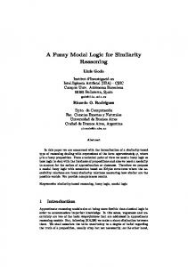
1.5.6 The S5-Cube Different combinations of modal axioms lead to different systems. If we take the modal system K and its axioms as foundation, we can simply add any combination of T, 4, D, B, and 5 to obtain different modal systems, of which KT4 corresponds to S4, and KT45 or KTB4 correspond to S5. The relation

between the different systems is usually illustrated as a cube as shown in Figure 1.4. Many combinations do not appear there, as these can be defined as other combinations which are shown, e.g., KB4 and KB5 describe the same logic, as well as KT45, KTB4, and KT5.19 17

Wijesekera [149] proposed Kripke semantics for a variant of CK before. Concerning the axioms, IK3 is kept and only IK4 and IK5 are dropped. Alternative special Kripke semantics for CS4 are proposed by Alechina et al. [4]. 18 see also [4, 110, 112, 132]. 19 The shown cube is based on that for the CK-family of [6]. A different one for the K-family can for example be found in [26]. Note that in the literature (also in [6, 24]) the letter ‘K’ is often omitted as K is an axiom of all the shown systems.

25

1 Introduction

S4

S5

KT

KTB KD4

KD45 KD5 KDB

KD K4

K45

KB5

K5 K

KB

Figure 1.4: The S5-Cube The same cube exists also for the IK-family. We simply prefix every modal system of the S5-cube with an ‘I’ [24]. This we call the IS5-cube. Accordingly, for the CK-family we prefix the systems with a ‘C’ and obtain the CS5-cube [6].

In order to check the equality of two logical systems one can show that the combination of frame properties in one system implies the properties of the other one and vice versa.

26

2 Sequent Systems and Dialogues

In the first part of this chapter, we consider different sequent systems, especially for classical and intuitionistic propositional logic (Section 2.1), as well as for several propositional modal logics (Section 2.2). There are different approaches which all have their own flavours, advantages or disadvantages. Dyckhoff [41] provides a historical overview of systems for intuitionistic propositional logic. For our purpose, we concentrate on proof searching issues and on systems which are relevant for the further progress of this work. There are, inter alia, calculi that embed λ-terms, making use of the CurryHoward isomorphism, which we do not discuss here. We also introduce a multi-conclusion calculus for the modal system CS4 (Section 2.2.2). In the second part, we turn to dialogical games and have a look at historical approaches of differend kinds. Most of these systems are related to intuitionistic and classical first-order logic. In Section 2.3 we focus on the propositional fragment (although we also have a short look at the first-order variants) and afterwards on several modal-logical approaches (Section 2.4). Finally, in Section 2.5, we point out similarities of sequent systems and dialogical calculi concerning proof-searching strategies.

27


2.1 Sequent Systems for Classical and Intuitionistic Logic 2.1.1 Gentzen’s Systems LK and LJ Sequent systems go back to Gerhard Gentzen. In [60] he presents the systems NJ and NK for natural deduction1 , as well as the systems LJ and LK which are usually called sequent systems. All four calculi are used to perform deduction in first-order logic. NJ and LJ are intuitionistic variants of NK and LK which are used for classical logic. As Gentzen states in [60], his natural deduction techniques provide a formal way of how a mathematical proof is usually done. LJ and LK are rather introduced to make it possible to formulate and prove his Hauptsatz, namely that it is possible to transform any formal proof to some normal form [60], which is the result of an admissible technique for sequent calculi that is nowadays widely known as cut elimination. Unless stated otherwise, for all sequent systems we consider in the following, it has been shown that the cut rules are dispensable with respect to completeness. In Gentzen’s systems LJ and LK, every state of a proof can be expressed as a sequent (that is where the name comes from) of the form A1 , A2 , . . . An ⇒ B1 , B2 , . . . Bm , so in each sequent we have two sequences (or lists) of formulas separated by the ⇒ symbol. The left sequence (the A’s) is called the antecedent of the sequent, the right part (the B’s) is called succedent [81]. In fact, the genV eral sequent from above can be read as the implication: from ni=1 Ai follows Wm j=1 Bj , or to express it in words: the conjunction of all antecedent formulas of a sequent implies the disjunction of all succedent formulas (of the sequent). 1

He gave the natural deduction system the German name Kalkul ¨ des naturlichen ¨ Schließens.

28

2.1 Sequent Systems for Classical and Intuitionistic Logic

We say that a sequent is derivable or valid, iff it is an axiom or it can be derived due to rules which a sequent system provides. For any arbitrary formula A, the sequent A⇒A is derivable/valid. This sequent is called an axiom (Anfangssequenz [60]). When we consider a sequent that is not an axiom, we have to apply rules2 to justify its validity. Applying such rules, one after another, leads to a derivation of a sequent by constructing a sequent tree. Gentzen distinguishes logical and structural rules. The former depend on the outer-most operator of some formula. The formulas of antecedent and succedent also refer to different sets of rules. We call rules for formulas of the antecedent left-hand rules or antecedent rules and those for formulas of the succedent right-hand rules or succedent rules. The differentiation between these sets is necessary as they have other semantic meanings, namely the antecedent sequents are interpreted as conjunctions and the succedent sequents as disjunctions. Structural rules are mainly used to add or remove formulas to/from sequences or to exchange the order of formulas within a sequence. As in Chapter 1.3.4, a rule consists of zero, one or two (or sometimes even more) premises which are in our case sequents written above a horizontal line, and exactly one conclusion below the line. For example, there are two rules for conjunction in the antecedent which look thus: A, Γ ⇒ Θ A ∧ B, Γ ⇒ Θ

B, Γ ⇒ Θ A ∧ B, Γ ⇒ Θ

Both rules have one premise. The Greek letters Γ and Θ stand for arbitrary (possibly empty) sequences of formulas. The sequence A, Γ is a sequence 2

Gentzen [60]: Schlußfigurenschemata

29


that starts with a formula A, which again stands for an arbitrary formula, and is continued by sequence Γ (see also Chapter 1.3). Rules can be interpreted as a deduction which says: if all premises are derivable/valid, then the conclusion is derivable/valid as well. In the first case from above, one could interpret the rule as: if A and the conjunction of all formulas of Γ imply the disjunction of formulas of Θ, then A ∧ B and the conjunction of all formulas of Γ imply the disjunction of formulas of Θ. To find a proof/deduction for a sequent, one usually applies the rules backwards, i.e., from bottom to top until one reaches axioms in all branches of the sequent tree. We say that a sequent tree is closed iff axioms occur at all its leaves. For the conjunction in the succedent, Gentzen provides only one sequent rule with two premises: Γ ⇒ Θ, A Γ ⇒ Θ, B Γ ⇒ Θ, A ∧ B Note that in general, antecedent rules operate on the first formula of the antecedent sequence and rules for the right-hand side on the last formula, respectively. In the displayed rule, the last formulas of the succedents are replaced (A and B are replaced by A ∧ B while Θ is left untouched). The formulas A and B are usually called active formulas.3 The result A ∧ B in the conclusion is called principal formula, and all other formulas of Γ and Θ are side formulas. In the following, when we say that a rule is applied, we refer to the principal formula and read the application from bottom to top. The application then results in the premise sequent(s) if the rule is not applied in an axiom sequent. As structural rules Gentzen provides three pairs plus the cut-rule. These are shown in Figure 2.1.4 He introduces two different sequent systems (LK 3

We use the terms proposed in [142]. Kleene [81] called the active formulas side formulas, while Troelstra and Schwichtenberg name the untouched formulas side formulas. 4 We use other symbols here to keep consistency with respect to the systems we consider later.

30


Weakening Γ ⇒ ∆ A, Γ ⇒ ∆

Γ ⇒ ∆ Γ ⇒ ∆, A

Contraction A, A, Γ ⇒ ∆ A, Γ ⇒ ∆

Γ ⇒ ∆, A, A Γ ⇒ ∆, A

Exchange Γ , A, B, Θ ⇒ ∆ Γ , B, A, Θ ⇒ ∆

Γ ⇒ ∆, A, B, Λ Γ ⇒ ∆, B, A, Λ

Cut Γ ⇒ ∆, A A, Θ ⇒ Λ Γ , Θ ⇒ ∆, Λ Figure 2.1: Structural Rules of Gentzen’s original sequent system

and LJ) that make it possible to derive statements, which are valid in the corresponding logic (classical or intuitionistic first-order logic), syntactically. This is simply done by applying the provided rules to obtain a sequent tree, where in each of its leaves an axiom sequent occurs. He uses the same logical and structural rules in both systems but puts a restriction to LJ on the meta level to comply with the intuitionistic semantics (more on this follows in the next section).

2.1.2 Getting Rid of Structural Rules Based on Gentzen’s LK and LJ, Kleene [81] introduced system G3 considering sequences to be equal iff they are cognate to each other, i.e., iff they simply contain the same formulas, no matter in which order. This makes the structural rules (with the exception of Cut) dispensable [81] and actually leads us to the use of multi-sets or sets instead of sequences.

31


P, Γ ⇒ ∆, P

ax

A, B, Γ ⇒ ∆ ∧l A ∧ B, Γ ⇒ ∆

⊥, Γ ⇒ ∆

⊥l

Γ ⇒ ∆, A Γ ⇒ ∆, B ∧r Γ ⇒ ∆, A ∧ B

A, Γ ⇒ ∆ B, Γ ⇒ ∆ ∨l A ∨ B, Γ ⇒ ∆

Γ ⇒ ∆, A, B ∨r Γ ⇒ ∆, A ∨ B

Γ ⇒ ∆, A B, Γ ⇒ ∆ ⊃l A ⊃ B, Γ ⇒ ∆

A, Γ ⇒ ∆, B ⊃r Γ ⇒ ∆, A ⊃ B

Γ ⇒ ∆, A ¬l ¬A, Γ ⇒ ∆ ∀x A, A[x/t], Γ ⇒ ∆ ∀l ∀x A, Γ ⇒ ∆ A[x/y], Γ ⇒ ∆ ∃l ∃x A, Γ ⇒ ∆

A, Γ ⇒ ∆ ¬r Γ ⇒ ∆, ¬A Γ ⇒ ∆, A[x/y] ∀r Γ ⇒ ∆, ∀x A Γ ⇒ ∆, A[x/t], ∃x A ∃r Γ ⇒ ∆, ∃x A

Figure 2.2: Rules of GCPC/G3c (c.f. [39, 142])

In the meantime, Ketonen [79] simplified some of Gentzen’s logical rules. Combining both alternations leads to systems like GCPC and GHPC by Dragalin [39] for classical and intuitionistic first-order logic respectively. Based on these, Troelstra and Schwichtenberg [142] present G3c and G3i. For each, soundness and completeness and the admissibility of cut-elimination5 , which says that the cut-rule (Figure 2.1) is dispensable, are shown. From now on, unless stated otherwise, we consider the Greek capital letters Γ and ∆ as multi-sets of formulas instead of sequences. The rules of GCPC/G3c6 are shown in Figure 2.2. For the rules ∀r and ∃l we have to make sure that the variable y does not occur as free variable (Eigenvariable) in the conclusion (c.f. [60, 39, 142]). The letter t stands for an arbitrary term. In the ax -rule P is an atomic formula.

5 6

This corresponds to Gentzen’s Hauptsatz. The systems GCPC and G3c are equal. However, GHPC and G3i have different sets of rules and are here considered separately.

32


P, Γ ⇒ P

ax

⊥, Γ ⇒ A

A, B, Γ ⇒ C ∧l A ∧ B, Γ ⇒ C A, Γ ⇒ C B, Γ ⇒ C ∨l A ∨ B, Γ ⇒ C

Γ ⇒A Γ ⇒B ∧r Γ ⇒A∧B Γ ⇒A ∨r Γ ⇒A∨B

A ⊃ B, Γ ⇒ A B, Γ ⇒ C ⊃l A ⊃ B, Γ ⇒ C ¬A, Γ ⇒ A ¬l ¬A, Γ ⇒ C ∀x A, A[x/t], Γ ⇒ C ∀l ∀x A, Γ ⇒ C A[x/y], Γ ⇒ C ∃l ∃x A, Γ ⇒ C

⊥l

Γ ⇒B ∨r Γ ⇒A∨B

A, Γ ⇒ B ⊃r Γ ⇒A⊃B A, Γ ⇒ ⊥ ¬r Γ ⇒ ¬A Γ ⇒ A[x/y] ∀r Γ ⇒ ∀x A Γ ⇒ A[x/t] ∃r Γ ⇒ ∃x A

Figure 2.3: Rules of G3i (c.f. [142])

So far, we have not made any distinction between LK and the intuitionistic version LJ. The reason is that the difference cannot be found in the rules themselves. Gentzen puts a restriction on a meta level: in every LJ sequent, the succedent may only contain one or no formula [60]. Considering the sequences as sets again, this leads us to system G3i, where this meta rule is implemented directly. The rules of G3i (in the variant we consider in the following) are displayed in Figure 2.3. The restrictions for the free variables are the same as in G3c. The differences are as follows: • The succedent of all sequents contains exactly one formula. This means

that we need two different rules for ∨r, one for the left and one for the right disjunct. • Reading the rules from bottom to top, in rule ⊃l, A ⊃ B is kept in the

left premise. Accordingly, ¬A is kept in the premise of rule ¬l.

33


Sequent systems in which the succedent contains at most one formula, like G3i, are called single-conclusion sequent systems or single-conclusion calculi. By contrast, if we permit more than one formula in the succedent, like in G3c, we say that the sequent calculus is a multi-conclusion sequent system or multiconclusion calculus. The requirement that the succedent of each sequent consists of only one formula makes it impossible to derive non-intuitionistic tautologies like the law of the excluded middle P ∨ ¬P: ⇒P ∨r ⇒ P ∨ ¬P

P ⇒ ⊥ ¬r ⇒ ¬P ∨r ⇒ P ∨ ¬P

Both of these derivations cannot be completed with a closing rule (ax or ⊥l). The reason is that when constructing the tree (reading it from bottom to top), resolving the ∨ forces us to drop one of the disjuncts which is needed to obtain the axiom sequent finally. By contrast, in GCPC/G3c, we can keep both disjuncts and the derivation closes: ax

P ⇒ P ¬r ⇒ P, ¬P ∨r ⇒ P ∨ ¬P The second difference between G3i and G3c, namely keeping the principal formula in the rules ⊃l and ¬l, is necessary to ensure completeness of the proof system.7 If we kept the left contraction rule (Figure 2.1) as non-dispensable, this measure would not be necessary, as it would be possible to duplicate formulas arbitrarily (reading the rules from bottom to top). Therefore, we call the rules ⊃l, ¬l and ∀l of G3i duplication rules. The duplication is only necessary because information is lost when some of the G3i-rules are applied, e.g., one disjunct is lost when we use ∨r. As such loss of information is restricted in G3c, duplication is only necessary in ∀l and ∃r there. 7

Note that negation is a special case of implication as ¬A can be written as A ⊃ ⊥.

34

2.1 Sequent Systems for Classical and Intuitionistic Logic ax

¬(P ∨ ¬P), P ⇒ P ∨r ¬(P ∨ ¬P), P ⇒ P ∨ ¬P ¬l ¬(P ∨ ¬P), P ⇒ ⊥ ¬r ¬(P ∨ ¬P) ⇒ ¬P ∨r ¬(P ∨ ¬P) ⇒ P ∨ ¬P ¬l ¬(P ∨ ¬P) ⇒ ⊥ Figure 2.4: Necessity of duplication in G3i

An example (mentioned in [40]) which shows the necessity of this duplication is shown in Figure 2.4. As it can be seen, the derivation is not possible if the principal formula ¬(P ∨ ¬P) is dropped from the premise of ¬l.

2.1.3 Multi-Conclusion Sequents for Intuitionistic Logic In 1954, Maehara [104] introduced a multi-conclusion version L’J of LJ that is actually based on LK, with the difference that the rules for ⊃r, ¬r and ∀r are replaced by variants in which the succedents of the premises are empty besides the active formulas. In other words, reading these rules from bottom to top again, formulas are dropped when they are applied. We call these rules critical [44] or non-invertible rules, while the others are called non-critical or invertible rules. More details follow in Chapter 3.3.1. Again, we consider a variant of L’J that gets along without the structural rules. This we call G3im which is based on Dragalin’s GHPC [39].8 The rules of G3im are the same as those of G3c with the exception that we replace rules ⊃l, ¬l, ⊃r, ¬r and ∀r by those shown in Figure 2.5. G3im is a multiconclusion version of G3i. In the following chapters, we make use of G3im at several points, so it has an important role in this work. Duplication is needed again in ⊃l and ¬l (and ∀l as before). To apply the rule ∀r, it must be ensured that y does not occur free in the conclusion [142]. 8

It is called m-G3i in [142] and LJmc in [44]. The difference to GHPC is explained below.

35


A ⊃ B, Γ ⇒ ∆, A B, Γ ⇒ ∆ ⊃l A ⊃ B, Γ ⇒ ∆ A, Γ ⇒ B ⊃r Γ ⇒ ∆, A ⊃ B

A, Γ ⇒ ∅ ¬r Γ ⇒ ∆, ¬A

¬A, Γ ⇒ ∆, A ¬l ¬A, Γ ⇒ ∆ Γ ⇒ A[x/y] ∀r Γ ⇒ ∆, ∀x A

Figure 2.5: Rules of G3im (c.f. [142])

The only difference to GHPC is the rule for ⊃l which differs from that of G3im in the conclusion of the left premise. By contrast to ⊃l of G3im , this is critical as well [39]: A ⊃ B, Γ ⇒ A B, Γ ⇒ ∆ ⊃l A ⊃ B, Γ ⇒ ∆ From now on we concentrate on propositional logic, because the main topic of this work is propositional modal logic, in which the quantifiers do not occur. Therefore, for the following sequent systems we do not consider the rules ∀l, ∀r, ∃l or ∃r anymore. Also, because ¬A is equal to A ⊃ ⊥9 some of the following calculi do not provide rules for the negation ¬.

2.1.4 Termination in Intuitionism We already observed that the duplications in ⊃l and ¬l are necessary in systems G3i and G3im for completeness. On the other hand, they are a problem: every non-duplicating rule (read from bottom to top) that is related to a logical connective, decomposes a formula which means that after a certain amount of rule applications, we finally obtain atomic formulas in the leaves of a proof tree. However, the duplication rules keep the principal formula in (at least) one premise which prevents the system to terminate when the conclusion sequent is not valid. 9

To verify this, we can use one of the systems from above to show that ¬A ⇒ A ⊃ ⊥ and A ⊃ ⊥ ⇒ ¬A are both valid sequents.

36


For example, let us consider Peirce’s Law ((P ⊃ Q) ⊃ P) ⊃ P. This formula is a tautology in classical propositional logic, but not in intuitionistic. Nevertheless, if we try to prove it in G3im , we obtain the following tree: ...

(P ⊃ Q) ⊃ P, P, P ⇒ Q ⊃r (P ⊃ Q) ⊃ P, P ⇒ Q, P ⊃ Q P, P ⇒ Q ⊃l (P ⊃ Q) ⊃ P, P ⇒ Q ⊃r (P ⊃ Q) ⊃ P ⇒ P, P ⊃ Q (P ⊃ Q) ⊃ P ⇒ P ⊃r ⇒ ((P ⊃ Q) ⊃ P) ⊃ P

P⇒P

ax

⊃l

At the position indicated by “. . . ” further rule applications of ⊃l are possible which would not help us to reach an axiom sequent anyway. We say that the proof does not terminate and therefore the systems G3i and G3im do not guarantee termination. If we have a closer look at the top left sequent of the tree, we see that actually no new information is added compared to two levels below. We only have one extra P in the antecedent. Although we could apply rules again and again, we would not gain any new facts. We actually have some kind of loop here which can be detected as recurrences within a tree [40]. However, if one wants to implement an automated theorem prover based on these sequent systems it will be helpful to have one that prevents such loops from the start using special rules. But of course, completeness and soundness must be preserved.

Implications in Detail

Dyckhoff [40] presents a variant of G3i he traces back to Vorob’ev [146] and which has been rediscovered by Hudelmaier [74]. The rule ⊃l is replaced by the four rules of Figure 2.6. Rule ⊃l1 may only be applied if P is atomic. Note that in this calculus negations ¬A are interpreted as implications A ⊃ ⊥. This system is often called G4ip10 ; in the following, we simply call it G4i.

37


B, P, Γ ⇒ D ⊃l1 [P is atomic] P ⊃ B, P, Γ ⇒ D A ⊃ C, B ⊃ C, Γ ⇒ D ⊃l3 (A ∨ B) ⊃ C, Γ ⇒ D

A ⊃ (B ⊃ C), Γ ⇒ D ⊃l2 (A ∧ B) ⊃ C, Γ ⇒ D

B ⊃ C, Γ ⇒ A ⊃ B C, Γ ⇒ D ⊃l4 (A ⊃ B) ⊃ C, Γ ⇒ D

Figure 2.6: Rules of G4i (c.f. [40]) If we try to prove Peirce’s Law in G4i, we obtain the following finite sequent tree where no further rule applications are possible: Q ⊃ P, P ⇒ Q ax ⊃r P⇒P Q⊃P⇒P⊃Q ⊃l4 (P ⊃ Q) ⊃ P ⇒ P ⊃r ⇒ ((P ⊃ Q) ⊃ P) ⊃ P This is the only possible saturated11 G4i-tree for Peirce’s Law, if P and Q are prime formulas. In G4i, termination is guaranteed [40]. From the proofsearcher’s point of view, the rules do not only take the outer-most operator of the principal formula into account, but consider also the structure of the principal’s antecedent. So we have four possibilities for this structure: it can be an atom (⊃l1 ), a conjunction (⊃l2 ), a disjunction (⊃l3 ), or an implication (⊃l4 ). When it is not an atom, the active formulas are in general new implications, which are not subformulas of the principal. However all rules of the other sequent systems considered so far have this subformula property which is given up in G4i [33, 32].

Rule Restrictions

Another approach which guarantees termination in intuitionistic propositional logic, is given by Corsi and Tassi. Their system IG [32, 33] is based on G3im , but has an additional rule named a fortiori: 10 11

The p indicates that only propositional formulas are considered in the system. i.e., no further rule applications are possible.

38


Γ ⇒ ∆, B a.f Γ ⇒ ∆, A ⊃ B This does not replace ⊃r. Instead, meta-rules (or external restrictions12 ) make clear in which case one may use ⊃r, a fortiori (a.f for short), or ⊃l to guarantee termination (adapted from [33]): i) Rule ⊃r may only be used once with the same principal formula within one path of the sequent tree. ii) If a formula A ⊃ B is principal in the application of a.f in a sequent tree t, then below this application in t, A ⊃ B is principal in an application of ⊃r on the same path. iii) If ⊃l is applied twice with the same principal A ⊃ B within one path of a sequent tree, then there is an application of ⊃r on the same path between these two ⊃l-applications. If these rules are obeyed, the IG-derivation is called to be regular, or IGr derivation for short. Considering any implication A ⊃ B on any path of a sequent tree from bottom to top, point i) ensures that ⊃r is only applied once with A ⊃ B as principal. Together with point iii), we may have ⊃l a limited number of times with the same principal. Trying to find a derivation for Peirce’s Law in IGr leads to the following tree: (P ⊃ Q) ⊃ P, P ⇒ Q, Q a.f (P ⊃ Q) ⊃ P, P ⇒ P ⊃ Q, Q P, P ⇒ Q ⊃l (P ⊃ Q) ⊃ P, P ⇒ Q ⊃r (P ⊃ Q) ⊃ P ⇒ P, P ⊃ Q (P ⊃ Q) ⊃ P ⇒ P ⊃r ⇒ ((P ⊃ Q) ⊃ P) ⊃ P

P⇒P

ax

⊃l

The leaves of this tree are blocked, i.e., no further rules can be used above. The reason is restriction iii): as there is no application of ⊃r above the second (read from bottom to top) application of ⊃l on (P ⊃ Q) ⊃ P, we are not 12

We say external because they are not implemented directly in the sequent rules.

39


allowed to put another ⊃l with the same principal on top. Using ⊃r instead of a.f is also not allowed because of restriction i). This is the only possible saturated IGr -tree for Peirce’s law with P and Q being prime formulas. IGr is sound and complete, and termination is guaranteed [32, 33]. The sub-formula property is preserved. The idea of enforcing termination with meta-rules suits game semantics well. In Chapter 3, we refer to IGr when establishing our intuitionistic multi-proponent dialectics with termination guarantee. An earlier calculus which guarantees termination in a similar way as IGr , is IPCRP (∧,⊃) by Heuerding et al. [68] which makes use of a history set that is extended in the left branch of ⊃l-applications. It is defined for the fragment of propositional intuitionistic logic having only ∧ and ⊃ as logical connectives. It was extended by Howe [73] to handle disjunctions (and negations) as well.13 It features also two versions of the ⊃r-rule (where one can be seen as a variant of a fortiori). Further restrictions are built into the rules themselves. We consider a variant for the modal logic S4 in Section 2.2.3. Howe himself also proposes an alternative approach making also use of history sets [72]. See [72, 73] for a detailed comparison. Another such system making use of some history-like set is proposed by Ferrari et al. [53]. In their work, there is only one left-hand rule and one right-hand rule for implication but the former has three premises instead of the usual two. The latter has two premises instead of one.

2.1.5 Focusing It is often the case that one can find different derivations for the same sequent in one and the same system, simply by reordering some rule applications or having applications which are not expedient for the derivation. For example, as we saw before, ⊃l can be applied infinitely often in G3i 13

Howe calls the method the Swiss history [73].

40


and G3im . To prevent such futile applications in proof searches, Andreoli [5] introduced a technique for linear logic called focusing. There are several adaptions for intuitionistic logic. Focusing enforces a normalization of sequent proofs. In Chapters 3 and 4, our aim will be to find normalized proofs with techniques of dialogical logic. Focused proofs are therefore relevant in this work although their strategy is different. Similarities and differences to multi-proponent dialectics are discussed in Section 3.4.2.

Uniform Proofs

Uniform proofs [114] were created to define behaviour of inference machines in logical programming languages and can be seen as early approaches of focused sequent systems (e.g., c.f. [96]). An intuitionistic single-conclusion sequent system is used as basis. Uniform proofs have the following restriction: if the succedent formula of a sequent is not atomic then it is principal of a rule application [114]. The result is that antecedent formulas can only be principal if a right-hand rule cannot be applied. However, this restriction is too strong and there is not a uniform proof for every valid sequent, for example ⇒ (A ∨ B) ⊃ (B ∨ A) cannot be derived with a uniform proof. Because of this incompleteness we do not consider uniform proofs further.

Isolating Critical Rule Applications

Searching for an isomorphism between special lambda-terms and proofs in sequent systems, Herbelin [66] introduced a simple focused system LJT for the fragment of intuitionistic logic having only the implication as possible connective. In this single-conclusion system, the sequents have the form

41


Γ; A ⇒ A

Γ , A; A ⇒ B Cont Γ , A; ⇒ B

ax

Γ; ⇒ A Γ; B ⇒ C ⊃l Γ; A ⊃ B ⇒ C

Γ , A; ⇒ B ⊃r Γ; ⇒ A ⊃ B

Figure 2.7: Rules of LJT (c.f. [66])

Γ; ⇒ C

or

Γ; A ⇒ C

i.e., it is possible to have a focused formula A in the antecedent which is explicitly separated from Γ due to a semicolon. This formula is called stoup [66].14 Before a rule can be applied on an implication of the antecedent, this principal needs to be stored to the stoup with a special kind of contraction rule (Cont). The rules of LJT are shown in Figure 2.7. Later, Herbelin introduced a sequent system LJQ which is based on G3i but has a restriction that says that above the left premise of ⊃l, only the rules ax , ∧r, ∨r and ⊃r are allowed [67]. This external restriction is internalized in the variants LJQ’ and LJQ∗ presented by Dyckhoff and Lengrand [42]. LJQ’ is a single-conclusion system in which two kinds of sequents are distinguished. The ordinary sequents have the usual form Γ ⇒ A with Γ being a multi-set. Focus sequents simply have another implication arrow (→ instead of ⇒). The new condition is that in a derivation tree, the conclusion of left-hand rule applications must always be an ordinary sequent, while the conclusion of right-hand rules and rule ax are always focus sequents. There is also a special rule Der (for dereliction [42]) to transform an ordinary sequent into a focused one (read from bottom to top). The rules of LJQ’ are displayed in Figure 2.8 (top). The sequent P ∨ Q → P ∨ Q is not derivable in LJQ’ [42], because ∨l can only be applied on ordinary sequents, but not in focus sequents. However, P ∨ Q ⇒ P ∨ Q is derivable, of course.

14

The term stoup in such a setting goes back to Girard [61] (c.f. [66]).

42


LJQ’ (single-conclusion)

⊥, Γ ⇒ A

Γ → A Der Γ ⇒A

⊥l

A ⊃ B, Γ → A B, Γ ⇒ C ⊃l A ⊃ B, Γ ⇒ C A, B, Γ ⇒ C ∧l A ∧ B, Γ ⇒ C A, Γ ⇒ C B, Γ ⇒ C ∨l A ∨ B, Γ ⇒ C

P, Γ → P

ax

A, Γ ⇒ B ⊃r Γ →A⊃B

Γ →A Γ →B ∧r Γ →A∧B Γ →A ∨r Γ →A∨B

Γ →B ∨r Γ →A∨B

LJQ∗ (multi-conclusion)

⊥, Γ ⇒ ∆

⊥l

Γ → A; ∆ Der Γ ⇒ A, ∆

A ⊃ B, Γ → A; ∅ B, Γ ⇒ ∆ ⊃l A ⊃ B, Γ ⇒ ∆ A, B, Γ ⇒ ∆ ∧l A ∧ B, Γ ⇒ ∆

P, Γ → P; ∆

ax

A, Γ ⇒ B ⊃r Γ → A ⊃ B; ∆

Γ → A; ∆ Γ → B; ∆ ∧r Γ → A ∧ B; ∆

A, Γ ⇒ ∆ B, Γ ⇒ ∆ ∨l A ∨ B, Γ ⇒ ∆

Γ ⇒ A, B, ∆ ∨r Γ → A ∨ B; ∆

Figure 2.8: Rules of LJQ’ and LJQ∗ (c.f. [42])

43


An important feature is that the left premise of ⊃l is a focus sequent which makes it impossible to have left-hand rule applications directly above. By contrast, the premise of ⊃r is an ordinary sequent again. The combination of both ensures that we can have ⊃l twice with the same principal formula (instance) on the same path of a proof tree only if there is an application of ⊃r in between. Dyckhoff and Lengrand also present system LJQ∗ [42] as a multi-conclusion variant of LJQ’ based on a system of the same name by Herbelin [67]. The focus sequents have now the form Γ → A; ∆ where the formula A is separated by the semicolon from ∆. Rules above such sequents must be right-hand rules with A as principal. These focused formulas are also called stoup (this time in the succedent). So changing from an ordinary sequent to a focus sequent (from bottom to top) requires to choose the right formula to put into focus. Also note that the left premise of ⊃l has an empty succedent (besides the stoup) which is similar to Dragalin’s ⊃l of GHPC [42]. For both systems LJQ’ and LJQ∗ , termination is not guaranteed, e.g., searching for a proof of Peirce’s Law leads to the same problems as in G3i and G3im .

Focus with Polarities

Liang and Miller introduced a general version of focusing sequent systems for intuitionistic and classical first-order logic [96, 97] which is based more on Andreoli’s attempt for linear logic and which makes use of polarities as in Girard’s work [61, 62]. Formulas can always be categorised according to their outermost connective into different polarities. These then define in which phase of the proof a rule can be applied to the formula. In the following, we have a look at their system LJF for intuitionistic logic but we consider only the propositional fragment to keep things simpler. In LJF all formulas either have a positive or a negative polarity, which is assigned according to the following rules [96]:

44


• Prime formulas have an arbitrary polarity (either positive or negative),

but the assignment must be consistent, i.e., once chosen, the atoms with the same name also have the same polarity. • Positive formulas are positive primes (P+ ), >, ⊥, disjunctions (A ∨ B),

and positive conjunctions (A ∧+ B). • Negative formulas are negative primes (P− ), implications (A ⊃ B), and

negative conjunctions (A ∧− B). Note that a negative polarity has nothing to do with negation. It is simply a categorisation which is related to invertibility of rule applications. In LJF, there are both positive and negative conjunctions. The different polarities increase flexibility so it is possible to embed other systems (like LJQ’) into LJF. Concerning provability, it does not matter which polarities are assigned to the different conjunctions, but the choice has an impact on the proof strategy, i.e., the structure of the proof tree. Therefore, for now we can assign polarities to conjunctions in an arbitrary fashion [96]. Liang and Miller define four types of sequents with two types of focus [96]. We call formulas of [Γ ] or [C] focus candidates as a focus can be put on these formulas in a sequent of type (ii): (i) [Γ ], Θ −→ C This sequent has no focus. C is either a formula C or a bracketed formula [C]. In such a sequent, principals can be formulas of Θ or C if it is not bracketed. (ii) [Γ ] −→ [C] This is a special variant of (i), where Θ is empty and C is bracketed. In this sequent, a focus can be selected, i.e., put on a formula of Γ or on C. A

(iii) [Γ ] −−→ [C] The focus is set on formula A which originates from the antecedent of some sequent below. A is the principal of the rule application above.

45


(iv) [Γ ] −A → The focus is set on formula A which originates from the succedent of some sequent below. A is the principal of the rule application above. The rules of LJF are shown in Figure 2.9. Formulas A+ and A− have positive or negative polarities respectively. P+ and P− are prime formulas. D= must be a formula of negative polarity or a prime formula of positive polarity, whereas E# is a positive formula or a negative prime (c.f. [96]). Rules I r and I l correspond to ax in G3i and are only applicable on atoms which are in focus. Foci can be put on negative focus candidates in the antecedent (F l), or on the positive focus candidate in the succedent (F r). After the polarity of the focused formula has changed, it can be taken out of focus again (R l, R r). Unfocused formulas of the antecedent which are negative, and positive prime formulas of the antecedent can become focus candidates ([ ]l). The same holds for positive formulas and negative primes of the succedent ([ ]r). As introduction rules, we have unfocused rules where the principal is not in focus (⊥l, >l, ∧+ l, ∧− r, ∨l, ⊃r), left-focus rules with a focused principal that originates from some antecedent (sequent type (iii) from above; ∧− l, ⊃l), and right-focus rules with a focused principal originating from the succedent (sequent type (iv) from above; >r, ∧+ r, ∨r). The following simple tree shows a derivation for Q ⊃ (P ⊃ (Q ∧ P)) in LJF. We give Q a positive polarity and P a negative one. The conjunction Q ∧ P is considered to be positive. Other assignments of polarities are possible as well but lead to other structures of the proof tree.

46


Decision/Reaction Rules A−

[A− , Γ ] −−→ [C] Fl [A− , Γ ] −→ [C]

[Γ ] −A+ → Fr [Γ ] −→ [A+ ]

[Γ ], A+ −→ [C]

[Γ ] −→ A− Rr [Γ ] −A− →

A+

Rl

[Γ ] −−→ [C] [D= , Γ ], Θ −→ C [ ]l [Γ ], Θ, D= −→ C

[Γ ], Θ −→ [E# ] [ ]r [Γ ], Θ −→ E#

Initial Rules [P+ , Γ ] −P+ →

Ir

P−

[Γ ] −→ [P− ]

Il

Introduction Rules [Γ ], Θ, ⊥ −→ C

B

A

[Γ ] −−→ [C] A∧− B

[Γ ] −−−→ [C]

[Γ ], Θ −→ C >l [Γ ], Θ, > −→ C

⊥l

∧ l −

[Γ ] −−→ [C] A∧− B

[Γ ] −−−→ [C]

∧− l

[Γ ], Θ, A, B −→ C ∧+ l [Γ ], Θ, A ∧+ B −→ C

B

[Γ ] −−→ [C] A⊃B

[Γ ] −−→ [C]

>r

[Γ ], Θ −→ A [Γ ], Θ −→ B − ∧ r [Γ ], Θ −→ A ∧− B [Γ ] −A → [Γ ] −B → + ∧ r [Γ ] −A∧+ B →

[Γ ], Θ, A −→ C [Γ ], Θ, B −→ C ∨l [Γ ], Θ, A ∨ B −→ C [Γ ] −A →

[Γ ] −> →

⊃l

[Γ ] −A → ∨r [Γ ] −A∨B →

[Γ ] −B → ∨r [Γ ] −A∨B →

[Γ ], Θ, A −→ B ⊃r [Γ ], Θ −→ A ⊃ B

Figure 2.9: Rules of LJF (c.f. [97]).

47

2 Sequent Systems and Dialogues Il P− [Q+ , P− ] −→ P− Fl [Q+ , P− ] −→ P− Ir Rr [Q+ , P− ] −Q+ → [Q+ , P− ] −P− → + ∧ r [Q+ , P− ] −Q+ ∧+ P− → Fr [Q+ , P− ] −→ [Q+ ∧+ P− ] [ ]r [Q+ , P− ] −→ Q+ ∧+ P− [ ]l [Q+ ], P− −→ Q+ ∧+ P− [ ]l [ ], Q+ , P− −→ Q+ ∧+ P− ⊃r [ ], Q+ −→ P− ⊃ (Q+ ∧+ P− ) ⊃r [ ] −→ Q+ ⊃ (P− ⊃ (Q+ ∧+ P− ))

Reading the proof from bottom to top, we first have to apply all rules until every formula is bracketed, so we can set a focus. We start with rule ⊃r being applied twice.15 Afterwards, every formula can be made a focus candidate ([ ]l, [ ]l, [ ]r) and we can set a focus. We set it on Q+ ∧+ P− (F r). Note that it would also be possible to choose P− , but this would make the proof terminate without success as no rule could be applied above. Afterwards, we apply ∧+ r on the focused conjunction. The left branch is finished immediately (I r), the right one is not, because the polarity of P− does not fit to the initial rule. So the focus needs to be changed: it is taken from P− , which is moved into the succedent (R r), and put on P− of the antecedent (F l) which finishes the proof. This simple example demonstrates how LJF is used. Further examples can be found in [96, 97]. As we see, the rules put strong restrictions on possible applications which leads to a normalization of proofs that depends only on the selection of polarities for atoms and conjunctions. However, an important observation is that proof-relevant decisions are not only made when the focus is selected, but also when rules ∧− l or ∨r are applied. Termination is not guaranteed, because focus candidates of the antecedent stay focus candidates, also after being put into focus. This also means that it is possible 15

In the succedent, only positive formulas and negative atoms can be bracketed, but implications are negative.

48


B−

[A+ ∧− B− , A+ ] −→ [B− ] A+ ∧− B−

Il

∧− l

[A+ ∧− B− , A+ ] −−−−−→ [B− ] Fl [A+ ∧− B− , A+ ] −→ [B− ] [ ]l [A+ ∧− B− ], A+ −→ [B− ] Rl A+ [A+ ∧− B− ] −−→ [B− ] ∧− l + − − + − − A ∧ B − [A ∧ B ] −−−−−→ [B ] Fl [A+ ∧− B− ] −→ [B− ] [ ]l, [ ]r [ ], A+ ∧− B− −→ B−

B−

[A+ ∧− B− ] −→ [B− ] A+ ∧− B−

Il

∧− l

[A ∧ B ] −−−−−→ [B ] Fl [A+ ∧− B− ] −→ [B− ] [ ]l, [ ]r [ ], A+ ∧− B− −→ B− +

−

−

−

Figure 2.10: LJF-Proofs with unnecessary rule applications (left) and without (right) to have rule applications in a proof tree which do not contribute to the proof progress in a reasonable way as the two derivation trees in Figure 2.10 show. LJF can be used to embed systems LJT, LJQ’ and uniform proofs by fixing the polarities of the formulas in a specific way. Details are given in [96, 97]. The authors also present a variant of LJF for classical logic, called LKF.

More on Foci

Simmons [134] introduces an extension of LJF where the order of rule applications in parts with unfocused sequents is fixed, and with a different treatment of atoms. Chaudhuri et al. [22] present a multi-focus sequent system for the linear logic MALL. Here, it is possible to put more than one formula into focus. A multi-focus system for classical first-order logic is proposed in [23]. We do not discuss these here.

2.1.6 Hypersequents in Intuitionistic Logic Avron [7] was the first to use hypersequents as reasoning systems for intermediate logics. These are logics lying between classical and intuitionistic logics,

49


i.e., in which the intuitionistic theorems hold but not necessarily all classical ones. In this context, hypersequents calculi for intuitionistic propositional ¨ logic have been proposed by Ciabattoni and Ferrari [27], and Fermuller [49]. In each node of the proof tree, instead of considering single sequents, we operate on sequences of sequents. For intermediate logics we can then have an interaction between these sequents of a hypersequent. Regarding intuitionistic logic, it is possible to duplicate a whole sequent before applying a non-invertible rule and still keep book of the result. Calculi using hypersequents are a useful tool for proof searches. In Section 2.3.5, we consider a multi-proponent dialogical system which is based on them. In general, hypersequents have the following form [7]: Γ1 ⇒ ∆1 | Γ2 ⇒ ∆2 | . . . | Γn ⇒ ∆n so they are simply sequences of ordinary (sub-)sequents separated by vertical bars, although we rather consider them here as (possibly empty) multisets. As meta-variables representing arbitrary hypersequents, we use the letters G and H. If G = Γ1 ⇒ ∆1 | . . . | Γn ⇒ ∆n and H = Γn+1 ⇒ ∆n+1 | . . . | Γm ⇒ ∆m , then G | H is defined as Γ1 ⇒ ∆1 | . . . | Γn ⇒ ∆n | Γn+1 ⇒ ∆n+1 | . . . | Γm ⇒ ∆m . To operate on hypersequents, we need structural external rules which allow us to duplicate sequents or drop them from a hypersequent. The structural external rules are displayed in Figure 2.11 together with the logical rules of ¨ the intuitionistic system HLI’ proposed by Fermuller [49]. We assume that the logical rules can be applied on any of the ordinary sequents, not only on the one written at the leftmost position of the hypersequent. This calculus has the advantage that we can duplicate an ordinary sequent and take out different decisions. For example, consider again the

50


External Structural Rules Γ ⇒C|Γ ⇒C|H EC Γ ⇒C|H

G EW G|H Axioms A, Γ ⇒ A | H

ax

⊥, Γ ⇒ C | H

⊥l

Logical Rules A, A ∨ B, Γ ⇒ C | H B, A ∨ B, Γ ⇒ C | H ∨l A ∨ B, Γ ⇒ C | H Γ ⇒A|H ∨r Γ ⇒A∨B|H A, A ∧ B, Γ ⇒ C | H ∧l A ∧ B, Γ ⇒ C | H

Γ ⇒B|H ∨r Γ ⇒A∨B|H B, A ∧ B, Γ ⇒ C | H ∧l A ∧ B, Γ ⇒ C | H

Γ ⇒A|H Γ ⇒B|H ∧r Γ ⇒A∧B|H A ⊃ B, Γ ⇒ A | H B, A ⊃ B, Γ ⇒ C | H ⊃l A ⊃ B, Γ ⇒ C | H

A, Γ ⇒ B | H ⊃r Γ ⇒A⊃B|H

Figure 2.11: Rules of HLI’ (c.f. [49])

51


law of the excluded middle of classical logic A ∨ ¬A which is not a theorem of intuitionistic logic:16 ⇒A | A⇒⊥ ¬r ⇒ A | ⇒ ¬A ∨r (twice) ⇒ A ∨ ¬A | ⇒ A ∨ ¬A EC ⇒ A ∨ ¬A Reading the tree from bottom to top, we first duplicate the sequent with the external contraction rule (EC ), because, as this is a single-conclusion calculus, we have to decide whether to keep the left or the right disjunct when using ∨r. Now we can look at both possibilities in parallel. As we are soon not able to do anything in the left sequent, we can apply ¬r in the right one which leads to a dead-end as well. There are several ways to put these sub-sequents together again in order to implement systems for different intermediate logics (e.g. c.f. [7, 28, 27]). To do reasoning in classical logic, we simply need to add the following rule:17 Γ, Γ 0 ⇒ A | H CL Γ ⇒ ⊥ | Γ0 ⇒ A | H So if one sub-sequent has ⊥ as succedent, it can be combined with another sub-sequent. This allows us to finish the derivation from above putting the following on the top: ax

A⇒A CL ⇒A | A⇒⊥ We consider such merging of sequents in the setting of dialogues briefly in Section 2.3.5. Hypersequents play also an important role in modal logic. 16 17

The example is adapted from [49]. The rule is taken from [28]. In [27] and [49], more general versions are used.

52

2.2 Sequent Systems for Modal Logic

A sequent system which uses sequent lists instead of hypersequents is SIC by Corsi and Tassi [33]. Instead of considering all individual sequents at the same time, only the last one of the sequent list is taken into account, which differs to hypersequents [33]. It makes use of the a fortiori rule and guarantees termination. Restrictions of IGr are directly implemented by using special labels attached to formulas. Nested sequents are an alternative to hypersequents where the nodes of the derivation tree do not contain hypersequents but the sequents have a nested structure. Fitting [58] provides such systems for both intuitionistic propositional and first-order logic. Lellmann [92] gives an alternative version, in which sequents are nested linearly. Both hypersequent and nested sequent calculi are also used to do reasoning in modal logics. More on this follows in Section 2.2.5. Next we consider various modal extensions of the propositional systems we examined so far, starting with the simple, ordinary sequent structures.

2.2 Sequent Systems for Modal Logic There are many sequent systems for modal logic as well. Early attempts like that by Curry [35] and Ohnishi and Matsumoto [117, 118] were presented before Kripke came up with his famous possible world semantics. There are too many of these calculi to discuss all of them here. We consider only a selection of systems in detail, which are relevant for our purposes. In particular, we concentrate on sequent systems for the logics K, KT and S4, and their intuitionistic/constructive variants. A survey of (unlabelled)

sequent calculi for normal modal logic can be found in [148] by Wansing. A more recent, general survey of sequent systems for normal modal logics, including Display calculus, is provided by Poggiolesi [123], which however does not cover standard hypersequents or focused sequents, but also takes

53


logics S5, GL and different combinations of axioms B, T and 4 into account. The reader is referred to her book for a detailed overview on calculi for classical modal logic.

2.2.1 Ordinary Modal Sequent Systems First, we have a look at modal extensions of the systems discussed in Sections 2.1.1 to 2.1.3. Like Wansing [148] and Poggiolesi [123], we call these ordinary sequent systems (not to mix up with ordinary sequents of focus calculi): all sequents have the simple structure Γ ⇒ ∆ where Γ and ∆ are either sequences, sets, or multi-sets of formulas. An early extension of Gentzen’s LK for modal logic K was proposed by Leivant [91] in 1981. He treats the sequences as sets and suggests to add a single rule: Γ ⇒A

2Γ ⇒ 2A

2I

There is no left- or right-hand rule for 2, but only this introduction. The set 2Γ is defined as {2φ | φ ∈ Γ }. Accordingly, we use this notation for other

sequent systems hereinafter, also we let 3∆ be {3φ | φ ∈ ∆}. In the succedent of Leivant’s rule, there is only a single formula both in the premise and in the conclusion. Therefore, when we use this rule in proof search, we have to make extensive use of the weakening rules, so that we have only boxed formulas in the antecedent, before we apply 2I. There is no rule for 3. Several years before, in 1957, Ohnishi and Matsumoto [117] presented rules for logics S4 (of which the 2-rules were already proposed earlier by Curry [34, 35]), T, and S5.18 Both left- and right-hand rules for 2 and 3 were introduced to extend LK. The additional rules for KT are 18

They use the name M for T and also propose rules for another modal system Q2 we do not consider here at all. For the S5 version, cut elimination does not work [87].

54


A, Γ ⇒ ∆ 2l 2A, Γ ⇒ ∆

Γ ⇒ A 2r 2Γ ⇒ 2A

A ⇒ ∆ 3l 3A ⇒ 3∆

Γ ⇒ ∆, A 3r Γ ⇒ ∆, 3A

2Γ ⇒ A 2r 2Γ ⇒ 2A

A ⇒ 3∆ 3l 3A ⇒ 3∆

Γ ⇒ ∆, A 3r Γ ⇒ ∆, 3A

and for S4 they are: A, Γ ⇒ ∆ 2l 2A, Γ ⇒ ∆

Differences between KT and S4 occur in rules 2r and 3l. Their application can be considered as changing the current world of the Kripke model. Note that these rules are based on LK and not on G3c. The contraction and weakening rules are required for certain derivations. Even worse, the systems are not complete, as for example, ¬2¬A ⊃ 3A cannot be shown to be valid [87]. Fitting [57] proposes a variant based on his tableau system. When applying his sequent rules, formulas of the conclusion are somehow kept in the premise, although he does not mention this explicitly. Contraction-free 2rules for K, KT and S4 can be found in [75], referring to [57]. These are as follows: Γ ⇒A 2K Γ 0 , 2Γ ⇒ ∆, 2A

Γ , 2A, A ⇒ ∆ 2T Γ , 2A ⇒ ∆

2Γ ⇒ A 24 Γ 0 , 2Γ ⇒ ∆, 2A

Note that Γ and Γ 0 are distinguished multi-sets. For modal logic K we use only rule 2K, for KT we use both 2K and 2T, and for S4 we forget about 2K and use both 2T and 24 instead [75]. The rules 2K and 24 can be seen

as right-hand rules for 2, while 2T is then the left-hand rule. The logic K therefore does not have a left-hand rule for 2. Analogous rules were already proposed by Kanger [78] in 1957 for KT and S4 (without adequateness proofs for the resulting systems). Due to the duality of 2 and 3, i.e., 2ϕ ≡ ¬3¬ϕ and 3ϕ ≡ ¬2¬ϕ, we can extend G3c by the rules shown in Figure 2.12 to obtain G3K for K, G3KT for KT, and G3S4 for S4.

The rules of G3S4 are exactly the same as those of G3s presented by Troelstra and Schwichtenberg [142]. The admissibility of the 3-rules in G3K and

55


G3K Γ ⇒ ∆, A 2r 2Γ , Γ ⇒ 3∆, ∆ 0 , 2A

A, Γ ⇒ ∆ 3l 3A, 2Γ , Γ 0 ⇒ 3∆, ∆ 0

0

G3KT 2A, A, Γ ⇒ ∆ 2l 2A, Γ ⇒ ∆

Γ ⇒ ∆, A 2r 2Γ , Γ ⇒ 3∆, ∆ 0 , 2A 0

A, Γ ⇒ ∆ 3l 3A, 2Γ , Γ 0 ⇒ 3∆, ∆ 0

Γ ⇒ ∆, 3A, A 3r Γ ⇒ ∆, 3A

G3S4 2A, A, Γ ⇒ ∆ 2l 2A, Γ ⇒ ∆

2Γ ⇒ 3∆, A 2r 2Γ , Γ 0 ⇒ 3∆, ∆ 0 , 2A

A, 2Γ ⇒ 3∆ 3l 3A, 2Γ , Γ 0 ⇒ 3∆, ∆ 0

Γ ⇒ ∆, 3A, A 3r Γ ⇒ ∆, 3A

Figure 2.12: Rules of G3K, G3KT and G3S4

G3KT can be shown easily due to the duality of the modal operators. Actually, these systems correspond to Fitting’s [57] analytic tableaux. Note that in all three cases, the rules 2r and 3l are non-invertible, as some formulas of the conclusions do not occur in the premises. Also, 2l and 3r are duplication rules, because the principal formulas stay in the premises. There are not many ordinary sequent systems for the intuitionistic modal logical counterparts IK/CK, IKT/CKT or IS4/CS4. For CS4, a single-conclusion system was created by Bierman and de Paiva [13]. We consider a slight variant of it proposed by Kuznets et al. [88] who also prove soundness and completeness of systems for CK, CKD (not considered here) and CKT.19 The rules consist of those of system G3i plus the corresponding modal rules displayed in Figure 2.13. 19

They refer to the cut-elimination techniques presented by Lellmann and Pattinson [93].

56


G3CK Γ ⇒A 2r 2Γ , Γ 0 ⇒ 2A

A, Γ ⇒ C 3l 3A, 2Γ , Γ 0 ⇒ 3C

G3CKT 2A, A, Γ ⇒ C 2l 2A, Γ ⇒ C

Γ ⇒A 2r 2Γ , Γ 0 ⇒ 2A

A, Γ ⇒ C 3l 3A, 2Γ , Γ 0 ⇒ 3C

Γ ⇒ A 3r Γ ⇒ 3A

2Γ ⇒ A 2r 2Γ , Γ 0 ⇒ 2A

A, 2Γ ⇒ 3C 3l 3A, 2Γ , Γ 0 ⇒ 3C

Γ ⇒ A 3r Γ ⇒ 3A

G3CS4 2A, A, Γ ⇒ C 2l 2A, Γ ⇒ C

Figure 2.13: Rules of G3CK, G3CKT and G3CS4 (c.f. [88])

A striking feature is that in all 3-rules, the succedent of the conclusion must be a 3-formula. The other rules are what we probably expect from an intuitionistic single-conclusion calculus. For the modal systems IK, IKT and IS4, I was not able to find an ordinary sequent calculus in the literature. It seems that it is not easy or even impossible to construct such systems, especially because of the IK5 axiom. Assume we have a single-conclusion sequent system for IK and we try do derive the corresponding formula: ax

B, A ⇒ B ⊃r B⇒A⊃B ??? 2r 3A ⊃ 2B ⇒ 3A 2B ⇒ 2(A ⊃ B) ⊃l 3A ⊃ 2B ⇒ 2(A ⊃ B) ⊃r ⇒ (3A ⊃ 2B) ⊃ 2(A ⊃ B) Of course, the left branch cannot be brought to an axiom. It is also no option to apply 2l instead of ⊃l as this would cause that 3A ⊃ 2B is dropped from the antecedent (change of Kripke world). Another possibility would be to set up an ordinary multi-conclusion calculus which results in thus:

57

2 Sequent Systems and Dialogues ax

B, A ⇒ B ⊃r B⇒A⊃B ??? 2r 3A ⊃ 2B ⇒ 2(A ⊃ B), 3A 2B ⇒ 2(A ⊃ B) ⊃l 3A ⊃ 2B ⇒ 2(A ⊃ B) ⊃r ⇒ (3A ⊃ 2B) ⊃ (2(A ⊃ B)) Now, of course it would be possible to apply 2r on top of the left branch and keep the A of 3A. But then there is actually no difference to the modal rules of G3K which would cause that 2 and 3 are dual (the sequent ⇒ ¬2¬A ⊃ 3A could be derived). The Kripke semantics of IK (p. 24) could make us believe that 2r is a critical rule.20 But if we then apply it on top of the left branch, the new premise would be ⇒ A ⊃ B for which there is also no derivation. Simpson [135] solves the problem with labels (see Section 2.2.4) but thereby leaves the area of ordinary sequent systems.

2.2.2 A Multi-Conclusion Sequent System for CS4 In this section, we introduce a cut-free multi-conclusion variant of G3iCS4. The reason is that the multi-proponent dialogues we consider in Chapter 4 are related to multi-conclusion sequent systems and the adequateness of the dialogical sequent system DiaSeqCS4, which we introduce in 4.2, is based on this. We call the following system G3iCS4m . The rules are displayed in Figure 2.14. Those of propositional logic are exactly the same as of G3im (Section 2.1.3). The new rules are 2l, 2r, 3l, and 3r, of which only 2l is invertible. Note that 3l can only be used when 3∆ is not empty.21 We show the adequateness of G3iCS4m by proving that every G3iCS4m -derivation can be M, w |= 2A holds iff for all refinements w 0 of w, in all successors u of w 0 , it holds M, u |= A. The reference to the refinements w 0 of w also occur for implication M, w |= A ⊃ B and negation M, w, |= ¬A. For both (and only for these) the right-hand rule is critical in G3im . 21 This restriction is added here next to the premise in the rule. We do not consider it as a premise in terms of derivation rules, but rather as an additional constraint.

20

58


P, Γ ⇒ ∆, P

ax

A, B, Γ ⇒ ∆ ∧l A ∧ B, Γ ⇒ ∆

⊥, Γ ⇒ ∆

Γ ⇒ ∆, A Γ ⇒ ∆, B ∧r Γ ⇒ ∆, A ∧ B

A, Γ ⇒ ∆ B, Γ ⇒ ∆ ∨l A ∨ B, Γ ⇒ ∆

Γ ⇒ ∆, A, B ∨r Γ ⇒ ∆, A ∨ B

A ⊃ B, Γ ⇒ ∆, A B, Γ ⇒ ∆ ⊃l A ⊃ B, Γ ⇒ ∆ ¬A, Γ ⇒ ∆, A ¬l ¬A, Γ ⇒ ∆ 2A, A, Γ ⇒ ∆ 2l 2A, Γ ⇒ ∆

⊥l

A, Γ ⇒ B ⊃r Γ ⇒A⊃B A, Γ ⇒ ∅ ¬r Γ ⇒ ∆, ¬A

2Γ ⇒ A 2r 2Γ , Γ 0 ⇒ 2A, ∆

|3∆| > 1 2Γ , A ⇒ 3∆ 3l 0 2Γ , Γ , 3A ⇒ 3∆, ∆ 0

Γ ⇒ A 3r Γ ⇒ 3A, ∆

Figure 2.14: Rules of G3iCS4m transformed into a G3CS4-derivation and vice-versa. Soundness and completeness of G3CS4 then imply soundness and completeness of G3iCS4m . Definition 2.1 (Deducibility (G3CS4, G3iCS4m )). For an arbitrary G3CS4/ G3iCS4m sequent Γ ⇒ ∆ we write for some n ∈ N: Sn Γ ⇒ ∆ iff there is a closed G3CS4-tree with Γ ⇒ ∆ as root sequent and which has a height h 6 n with m n ∈ N. We write M n Γ ⇒ ∆ iff there is a closed G3iCS4 -tree with Γ ⇒ ∆ as root

sequent and which has a height h 6 n. We also say that Γ ⇒ ∆ is deducible in n deductive steps, or that there is a derivation of height n for Γ ⇒ ∆. The S in Sn refers to single-conclusion and the M to multi-conclusion.

59


Lemma 2.1 (Admissibility of Weakening (G3CS4, G3iCS4m )22 ). For all ϕ, Γ , ∆: 1. If Sn Γ ⇒ ∆ then Sn Γ , ϕ ⇒ ∆. M 2. If M n Γ ⇒ ∆ then n Γ , ϕ ⇒ ∆. M 3. If M n Γ ⇒ ∆ then n Γ ⇒ ϕ, ∆.

The proof of this lemma is omitted here, as we discuss weakening in more detail in Chapters 3.3.1, 4.3.2, and 4.3.3.

Theorem 2.1 (G3iCS4m Completeness). Every G3CS4 proof tree can be transformed into a G3iCS4m proof tree. Proof. We consider the G3CS4-derivation Sn Γ ⇒ C with Γ being an arbitrary multi-set of formulas and C a single formula. We want to show that for some m and for all ∆ it holds: M m Γ ⇒ C, ∆. We perform an induction on n. Base Case: n = 1 — The only rule which is used in the derivation is either ax or ⊥l. • If the rule is ax , the root sequent has the form Γ , P ⇒ P. The rule ax

of G3iCS4m can also be used in the sequent Γ , P ⇒ P, ∆, so this is no problem. • The case of ⊥l works accordingly.

Inductive Step: Assume we have a G3CS4-derivation Sn+1 Γ ⇒ C. We have to perform a case analysis on the rule which is applied in the root sequent, i.e., the lowest rule application in the tree. We consider three cases here. The others are handled similarly. 22

The lemma is adapted from [39] and [142].

60


1. Assume that C is a disjunction A ∨ B with arbitrary formulas A and B. Also assume that A ∨ B is the principal formula of the lowest rule application. Then we have either Sn Γ ⇒ A or Sn Γ ⇒ B. By hypothesis, we obtain M m Γ ⇒ A, ∆ (or with B instead of A respectively). Then by weakening we achieve M m Γ ⇒ A, B, ∆. Now we append the application of ∧r below and get M m+1 Γ ⇒ A ∧ B, ∆ as root. 2. Assume that Sn+1 2Γ , Γ 0 ⇒ 2A and 2A is the principal.

Then

Sn 2Γ ⇒ A. By hypothesis, we then get M m 2Γ ⇒ A for ∆ = ∅. Ap0 pending 2r of G3iCS4m results in M m+1 2Γ , Γ ⇒ 2A, ∆ for an arbitrary

∆. 3. Assume that Sn+1 2Γ , Γ 0 , 3A ⇒ 3C and 3A is the principal of the low0 est rule application. We want to have M m+1 2Γ , Γ , 3A ⇒ 3C, ∆. We

define 3∆ 0 as the part of ∆ which contains 3-formulas, and let ∆ 00 be the rest. Then from Sn 2Γ , A ⇒ 3C we get by hypothesis: m 0

M m 2Γ , A ⇒ 3C, 3∆ and adding 3l of G3iCS4 leads to 0 0 00

M m+1 2Γ , Γ , 3A ⇒ 3C, 3∆ , ∆ .

For the transformation from multi-conclusion to single-conclusion sequents we adapt the technique by Maehara [104]. Assume that ∆ is the multi-set of W formulas δ1 , δ2 , . . . , δn . Then the disjunction over ∆, written ∆, is defined as δ1 ∨ δ2 ∨ · · · ∨ δn . We also need an additional lemma.

Lemma 2.2 (Alternative Succedents in G3CS4). For any Γ , n, and formulas A and B: if Sn Γ ⇒ A ∨ B, then Sn Γ ⇒ A or Sn Γ ⇒ B. Proof. By induction on n: Base Case: n = 1 — In this case, the only rule application in the derivation must be ⊥l, which can also be applied in Γ ⇒ A and Γ ⇒ B.

61


Inductive Step: We consider the lowest rule application of the derivation tree for Sn+1 Γ ⇒ A ∨ B. • If it is an application of ∧l, ∨l, or 2l, we can simply apply the hy-

pothesis on the premise of the application and append it afterwards again. • If it is an application of ⊃l on some formula C ⊃ D, then we have

Sn Γ , C ⊃ D ⇒ C and Sn Γ , D ⇒ A ∨ B. By hypothesis then Sn Γ , D ⇒ A or Sn Γ , D ⇒ B. Therefore, appending ⊃l again results in Sn+1 Γ , C ⊃ D ⇒ A or Sn+1 Γ , C ⊃ D ⇒ B. • The case of a ¬l-application works accordingly. • The only other possibility is an application of ∨r, but both thinkable

premises fulfil our target properties.

Theorem 2.2 (G3iCS4m Soundness). Every G3iCS4m proof tree can be transformed into a G3CS4 proof tree. Proof. What we have to show is that for any n, Γ , and ∆: M n Γ ⇒ ∆ implies W for some m: Sm Γ ⇒ ∆. We do this by induction on n. Base Case: n = 1 — We have two possibilities: • The only rule application is ax in a sequent such that M 1 Γ , P ⇒ P , ∆.

This corresponds to Sm Γ , P ⇒ P ∨

W ∆. There is obviously such a

derivation: we simply make use of ∨r and ax of G3CS4 and obtain the following tree: ax

Γ, P ⇒ P W ∨r Γ, P ⇒ P ∨ ∆ If P is not the left-most disjunct we simply make use of ∨r several times W until it is dissolved out of ∆.

62


• The only rule application is ⊥l. Then ⊥l can also be applied directly in

the sequent of G3CS4. Inductive Step: We have a look at three cases: 1. Assume M n+1 Γ ⇒ A ∨ B, ∆ with the lowest rule application being ∨r applied on A ∨ B. Then M n Γ ⇒ A, B, ∆. By hypothesis, this corresW ponds to Sm Γ ⇒ A ∨ B ∨ ∆. This is already what we were looking for.23 2. Assume M n+1 Γ , A ⊃ B ⇒ ∆ with the lowest rule application being ⊃l M applied on A ⊃ B. Then M n Γ , A ⊃ B ⇒ A, ∆ and n Γ , B ⇒ ∆. By W hypothesis then for some l and m: Sl Γ , A ⊃ B ⇒ A ∨ ∆ and W

Sm Γ , B ⇒ ∆. According to Lemma 2.2, the former leads us to two W cases: either Sl Γ , A ⊃ B ⇒ A or Sl Γ , A ⊃ B ⇒ ∆.

• If Sl Γ , A ⊃ B ⇒ A, then together with Sm Γ , B ⇒

⊃l to obtain Γ , A ⊃ B ⇒ • If Sl Γ , A ⊃ B ⇒

W ∆, we can use

W ∆.

W ∆, we are already finished.

0 0 3. Assume M n+1 2Γ , Γ , 3A ⇒ 3∆, ∆ and the lowest applied rule is 3l (on 3A). Then due to the premise we get M n 2Γ , A ⇒ 3∆ with |3∆| > 1, W and by hypothesis Sm 2Γ , A ⇒ 3∆ for some m.

• If

3∆ contains only a single disjunct, i.e., is some 3C, then we

W

can simply put 3l below and append

W 0 ∆ with rule ∨r.

• If it contains more than one disjunct, we apply Lemma 2.2 (if ne-

cessary multiple times) and locate the one which is relevant for the derivation. We call it 3E. Then it is again easy to build the root of the G3CS4-derivation:

23

Note that this requires that associativity of ‘∨’ is admissible in the succedent of any G3CS4-sequent. However, using Lemma 2.2 makes it possible to show easily that

Sn Γ ⇒ A ∨ (B ∨ C) iff Sm Γ ⇒ (A ∨ B) ∨ C.

63


⇒ Σ ; P, ¬P, ∆

ax

⇒ Σ ; A, B, ∆ ∨ ⇒ Σ ; A ∨ B, ∆

⇒ 3A, Σ ; A, ∆ 3 ⇒ Σ ; 3A, ∆

⇒ Σ ; A, ∆ ⇒ Σ ; B, ∆ ∧ ⇒ Σ ; A ∧ B, ∆ ⇒ ∅ ; A, Σ 2 ⇒ 3Σ ; 2A, ∆

Figure 2.15: Rules of KTSU (c.f. [68]) ... 2Γ , A ⇒ 3E 3l 2Γ , Γ 0 , 3A ⇒ 3E W ∨r (multiple times) 2Γ , Γ 0 , 3A ⇒ 3∆ W W ∨r (multiple times) 2Γ , Γ 0 , 3A ⇒ 3∆ ∨ ∆ 0

2.2.3 Termination in Modal Proof Search Like rule ⊃l in G3i, rules 2l and 3r of G3KT and G3S4 are duplication rules which might cause non-termination when searching for a proof, because these rules can be applied infinitely often on the same principal. Heuerding et al. [68] provide single-sided sequent systems, i.e., the sequents’ antecedents are always empty. Formulas are only handled when they are in negation normal form, which is no problem, as in classical modal logic it is possible to translate every formula into negation normal form. The axiom rule is then applied if there is a contradiction with respect to some atom in the sequent. The authors use separate multi-sets Σ and H for keeping book of certain formulas on which rules have already been applied [68]. The following systems by Heuerding et al. are based on algorithmic approaches by Ladner [89]. In system KTSU for the modal logic KT, H is not yet used. The rules (in our altered notation) are displayed in Figure 2.15. In rule ax , P is an atom. The only duplicating rule (3) adds the principal formula to Σ and prevents us to apply this rule on the same formula again, until we use the 2-rule. This

64


⇒ H ; Σ ; P, ¬P, ∆ ⇒ H ; Σ ; A, B, ∆ ∨ ⇒ H ; Σ ; A ∨ B, ∆ ⇒ ∅ ; 3A, Σ ; A, ∆ 3 0 ⇒ H ; Σ ; 3A, ∆

ax

⇒ H ; Σ ; A, ∆ ⇒ H ; Σ ; B, ∆ ∧ ⇒ H ; Σ ; A ∧ B, ∆

⇒ H ; Σ ; A, ∆ 3 1 ⇒ H ; Σ ; 3A, ∆

⇒ A, Θ, H ; Σ ; A, Σ 2 ⇒ H ; Σ ; 2A, 2Θ, ∆

Figure 2.16: Rules of KS4SU (c.f. [68]) corresponds to a world change in the Kripke model and moves the formulas out of the separated multi-set (the prefixed 3’s removed). So a repetition is also possible if it is done above the application of the non-invertible 2-rule, which is however enough for KT to terminate the proof search [68]. For S4, things are not that easy, as an additional history (multi-)set is needed. The rules for KS4SU are shown in Figure 2.16. The calculus has two rules for 3 and restrictions for rule applications are as follows (c.f. [68]): • Rule 30 may only be applied if 3A 6∈ Σ. • Rule 31 may only be applied if 3A ∈ Σ. • Rule 2 may only be applied if A 6∈ H.

As before, rule 2 causes a world change in the Kripke model. It is the only rule that extends the history H. The use of 30 empties the history, further applications on the same principal (with 31 ) do not touch H. System KS4SU is sound and complete and termination is guaranteed [68]. Howe [73] uses two separate history sets to set up a sequent system for the 2-fragment24 IS42 [12] of IS4/CS4.25 Another, more recent terminating se-

quent system for S4 is proposed by Fiorentini [54]. It deals with an extended 2-fragment means that the 3 is not considered to be part of the language, whereas the 2 and the propositional connectives are. 25 Howe states that he considers IS4, but when the 3 is not taken into account as an admissible operator, there is no difference between IS4 and CS4, as axioms IK2 to IK5 contain 3-formulas, and are therefore dropped anyway. The relevant axioms of IS42 are given in [12]. 24

65


modal language (two extra modalities) and so-called cluster-sequents which go beyond the scope of this work.

2.2.4 Labelled Modal Sequent Systems Instead of dropping formulas from sequents when non-invertible rules are applied, formulas can be equipped by labels, which refer to Kripke worlds, in which the corresponding formulas shall hold. When the relations are also added explicitly to the sequents, a single sequent can represent a whole Kripke model. One of the first labelled sequent systems for modal logics is presented by Mints [115] for modal logics K, KT, K4, KB, KTB, S4, and S5. Instead of labelling single formulas, he considers several sequents at once, i.e., sequences of labelled sequents. Whenever rule 2r is applied, a new sequent with a new label, representing a new Kripke world, is added. Vigano` [145] made the relational structure explicit. He introduced relational formulas of the form xRy, indicating the accessibility between two worlds x and y via a relation R. A labelled sequent then has either the form Γ , ρ ⇒ ∆ or ρ ⇒ xRy, where Γ and ∆ are multi-sets of labelled formulas and ρ is a multi-set of relational formulas. The second kind of sequent (relational sequents) is only used to reason about the relational structure of the model ` sequent systems, the 2r rule which is internally constructed. In Vigano’s adds relational formulas to the sequents, while above 2l we need to give reason that some relational formula can be derived. For these we then have different possibilities according to the corresponding modal system’s frame properties (which depend on the modal system) with additional rules. A cut rule is not provided. In [116] Negri presents similar rules without using relational sequents. In this simplification, sequents have the form Γ ⇒ ∆ with Γ now containing both labelled and relational formulas. In the following, we refer to Negri’s

66


sequent calculi as G3Kl , G3KTl , and G3S4l . Several years before, Simpson [135] introduced a labelled single-conclusion sequent calculus for IK with an additional general rule that can be used to include different frame properties, including reflexivity and transitivity. Adding such labels to the syntax of formulas leads us to hybrid logics, for which there are several sequent systems, e.g., proposed in [14, 17]. However, hybrid logic is a topic of its own and we do not discuss it hereinafter. Systems with labelled sequents are more flexible than the ordinary ones, as one can cope with different frame properties using rules that are applied on relational formulas. These rules can simply be added or removed to the basic set, instead of replacing 2- and 3-rules as in ordinary sequents. Further, it is possible to cope with modal logics like S5, for which there are only quite complex or no adequate ordinary systems at all, in an easy way. As Negri [116] states, all her rules are invertible, which is not the case for ordinary systems.

2.2.5 Avoiding Explicit Relations Hypersequents

Labelled systems as those we just considered, strongly rely on Kripke semantics, which is seen as a problem by some authors.26 This is one of the reasons why Avron [7] proposed a hypersequent system for S5. An earlier approach was proposed in an abstract by Pottinger [124] for logics KT and S4, where sequents consist of sequences instead of multi-sets.

Lahav [90] provides a method of how to transform frame properties to hypersequent rules, and thereby obtains calculi for a bunch of classical modal logics, inter alia for K, KT and S4. 26

A discussion on this topic can for example be found in [7], and Chapter 1.9 of [123].

67


Nested Sequents

Another similar possibility to hide the relational Kripke structure is the usage of nested sequents. These are often used as single-sided sequents, i.e., multisets, that contain formulas and again other nested sequents. Due to this structure, it is possible to map the frame of an underlying model without the usage of labels or relational formulas. ¨ Brunnler [19] provides a flexible system for the most common classical modal logics, inter alia K, KT, S4, S5. . . , where every frame property has its own rule. He states that for some combinations of frame properties his system is not cut-free. Poggiolesi introduces independently the similar method of tree-hypersequents for K, KD, K4, and KD4 [122], which she later extends for all modal systems of the S5-cube (not cut-free for K5 and not complete for KT5) [123].

Nested sequent systems for the intuitionistic modal logic IK with combinations of the extensions D, T, B, 4, and 5 are presented by Straßburger [141] and Marin and Straßburger [107]. All formulas of a single-sided nested sequent either have an input polarity corresponding to left-hand formulas of two-sided sequents, or an output polarity which can be seen as the right-hand formula, of which there is only one in each sequent. So the system can be considered as a single-conclusion calculus. It was later modified by Arisaka et al. [6] for the logics of the CS5-cube. An earlier approach for multi-modal CK, which can be interpreted as a special case of nested sequents, is the multi-conclusion sequent calculus without cut rule by Mendler and Scheele [112], based on the so-called 2-sequent calculus by Masini [108]. Here, the antecedent and the succedent of a sequent are departed into several sections, each representing another Kripke world. Linear nested sequents for the classical modal logics of the S4-cube (S5-cube without combinations of B or 5) plus combinations with 45 are provided by Lellmann [92].

68


Looking just one step ahead

It is worth to note Cerrato’s calculus [21] for all logics of the S5-cube, in which formulas can be bracketed with [ ] and h i to mark that all of them ([ ]) or one of them (h i) is valid in a succeeding world. When all formulas of a sequent are bracketed, further rules can then be used to move to there, dropping all these brackets. Cut-elimination is only shown for the K-case. A similar idea let Mendler and Scheele [111] introduce a calculus (without cut-rule) for the constructive description logic cALC, a syntactic variant of multi-modal CK.27

2.2.6 Focusing and Modal Logic As for propositional intuitionistic logic and linear logic, there are also some focusing attempts for modal logics. Miller and Volpe [113] transform LKF (Section 2.1.5) to a single-sided focused sequent system LMF for logic K. They exploit the fact that modal formulas can be translated to first-order formulas.

The usage of this

standard translation has the side effect that negated relational atoms may occur in the sequents. Other (classical) modal systems can be obtained by embedding rules which correspond to the frame properties [113]. Chaudhuri et al. present a focusing nested sequent calculus for the classical modal logics of the S5-cube [25], as well as for the logics of the IS5-cube [24] based on the calculus of [141]. Lellmann and Pimentel [94] provide a focusing version of the linear nested sequents for classical modal logics [92] mentioned above. However, I was not able to find a focusing calculus which is based on ordinary modal sequent systems, the simplest kind of modal sequent systems. Instead, those with focus found in literature make use 27

The authors state that cALC is “related to” CK as the standard logic of description logic, ALC, “is related to” K [111].

69


of labels or nested sequents. Also, there is currently no focusing calculus dealing with logics of the CK-family.

2.3 Lorenzen Dialogues as Proof Systems for Classical and Intuitionistic Logic It is now time to leave sequent systems and turn to dialogical games in more detail. In this section we discuss dialogues which can be used as proof systems for classical and intuitionistic logic. We consider several approaches with different advantages and disadvantages. Some of them deal with firstorder logic, while others are restricted to propositional logic. The former is of minor interest for this work, but these dialogues are the original ones and also have some features which will be useful when we turn towards modal logic in Section 2.4.

2.3.1 Preliminaries Here, we only give informal definitions for dialogues to illustrate the idea of the methodology and because in the literature the game rules are also often defined informally. We do not want to prove validity or other properties of the dialogical systems presented in this chapter. Later, when the multiproponent reasoning procedure is constructed in Chapters 3 and 4, we get more concrete and formal. Different mathematical definitions for dialogues and their rules can for example be found in [80, 47, 48, 143, 140]. Lorenzen first presented his ideas of dialogues in 1958 [100]. He argues that using the logical connectives in a way that corresponds to some —as he claims— natural meanings in a dialogue, leads to a proof system for intuitionistic logic [101]. At the beginning of a dialogue one of the two players, the proponent P, states a hypothesis in terms of a formula. The other player

70

2.3 Lorenzen Dialogues as Proof Systems for Classical and Intuitionistic Logic

who is called opponent O attacks this formula according to some predefined rules. P may then defend against this attack with a new formula and the game continues. Instead of defending, it is often also possible to counterattack a previous assertion of the attacking player. A dialogical game or run is a sequence of moves, each performed by one player. A move can be an attack, a defence, or the claim of the hypothesis. Further, a move is either an assertion which is a formula of some language, or a demand which we indicate with a question mark (?) and some additional symbol specifying the type of attack. An assertion stated by O is also called commitment or concession. Sometimes we allow O to state one or more concessions before P claims the hypothesis. These are called initial concessions and P can make use of them during the game as if they were stated then. A closed round as we consider it in this chapter for two-player dialogues, consists of two moves, namely one attack and one defence against this attack. A round in a game is open iff it consists of an attack but there is no corresponding defence. A p-strategy of a player p ∈ {O, P} is a function that defines the next move of p in a given non-empty game. The move needs to comply with the game rules. The strategy can therefore be seen as the player’s mind that leads him through the game. In general, a player wins a game, if the other one is not able to move anymore. A p-strategy is a p-winning-strategy iff, when consecutively applied, it makes p win the game, no matter what the other player’s moves are or will be. So, if a player has a winning strategy, he is always capable to win the game.

71


Assert A ∧ B A ∨ B A ⊃ B ¬A ∀x A ∃x A Attack ?l ? r ?∨ A A ?t ?∃ B — A[x/t] A[x/t] Defence A B A B Figure 2.17: Particle Rules for the First-Order Language based on [98]

2.3.2 D-Dialogues, E-Dialogues, and Ipse Dixisti for Validity Lorenz [98] defined the game rules for systems we call (as Felscher [47]) D-dialogues in the following. He considers two separate sets: the particle rules (allgemeine Spielregel28 ) define how to handle compound formulas locally, while the structural rules (spezielle Spielregel29 ) concern the players’ assertions globally [98], i.e., they define which player may move in which situation and also when a game finishes and who the winner is. Lorenz presents the particle rules for the first-order language in the form of a table. Figure 2.17 shows the rules in a slightly modified notation to serve our purpose. The letters A and B represent arbitrary first-order-formulas, x is a variable and t is an object [98] or term [47, 48]. As before, we write A[x/t] to express a substitution, where all occurrences of x in A are replaced by t. The first line of the table shows possible assertions that can be stated by one of the players. The second line defines how the other player can attack an assertion of the form given in the first line, while the last line expresses how to defend against the corresponding attack. The symbols ?∨ , ?l , ?r , ?t , and ?∃ are the demands. For example, if one player states a conjunction A ∧ B, then the other one can attack it with one of the demands ?l or ?r , asking the first player to defend either with the left or the right conjunct. The attacked player can then react 28

German for general game rule. In [47, 48] the rules are named argumentation forms, in [10] strip rules. We follow Lorenz’s later terminology and call them particle rules (German: Partikelregeln) [99]. 29 German for special game rule. Also called Rahmenregel [99] (German: frame rule). We follow Rahman and Keiff [127] and call them structural rules.

72


to this with the defence by stating the corresponding part of the previous assertion, i.e., with A or B respectively. A disjunction A∨B can only be attacked with ?∨ , while the defending player may choose whether to defend with the left or the right disjunct. An implication A ⊃ B is attacked by stating the antecedent A and defended with the consequent B. A negation ¬A is attacked directly due to the contrary statement A. Such an attack cannot be defended. When a universal statement ∀x A is given, then the attacking player may choose an object/term t, which must be used by the defender to give a concrete instance, i.e., by means of a substitution of x with t. For the existential statement ∃x A the defender may choose the object t for which he/she claims the assertion A. In a variant of the particle rules, Felscher [47, 48] adds a player variable to each statement indicating that the attacking and the defending player are different and that the attacking player always attacks statements by the other one.

D-Dialogues

When P is supposed to show general validity of his hypothesis, then the following rule has to be obeyed (called characteristic rule, “charakteristische Spielregel” [98]): (D0) P may state a prime formula only if it was stated by O before.

Further, Lorenz proposes the following structural rules for intuitionistic dialogues (“effektive Spielregel”) [98]:30 (D1O) An assertion by P may be attacked once in any following move. (D2P) An assertion by O may be attacked arbitrarily often in any following

move. 30

As we do not rely on his terminology or definitions here, the rules are paraphrased to simply give the main idea.

73


(D3) A defence may take place once and only if all rounds after the corres-

ponding attack are closed. Rule (D3) can also be seen as restriction, that players may only defend against the last open attack, i.e., the last attack by the other player for which there has been no defence yet [127]. As Felscher we call these rules D-rules and dialogues obeying them D-dialogues (c.f. Felscher [47, 48]). Also classical rules are presented, for which rule (D3) is replaced by the following [98]: (D3O) O may defend an assertion only if all rounds after the corresponding

attack are closed. (D3P) An assertion by P may be defended arbitrarily often in a following

move, once in an attack round if all rounds after the corresponding attack are closed, or in any following defence round. Here, attack rounds are the usual rounds consisting of an attack and a defence. By contrast, a defence round consists of a single defence against an attack which has already been defended before [98]. Later, Lorenz modifies the structural rules, making things more concrete. He defines who is the winner of the game (the last one who can perform a move), who begins, and so forth [99]. The particle rules are then included as part of the structural rules. Lorenz also introduces ranks (Schranken) which we discuss later in Section 2.3.4. We have a look at a simple example which is often used in the literature to show how dialogues work (first published in a similar way in [101]). It shows that P does not have a winning strategy for the formula A ∨ ¬A in intuitionistic dialogues. We assume that A is a propositional variable and therefore a prime formula. Figure 2.18 shows a dialogue tableau for this hypothesis. Different styles of such tableaux are proposed in the literature, e.g., [101, 98, 10, 127]. Our variant is a table consisting of three columns. The

74


O

P

1 A ∨ ¬A 2 [?, 1] ?∨ [!, 2] ¬A 3 [?, 2] A — — Figure 2.18: The Excluded Middle in an intuitionistic dialogue

first contains the row numbers, the second moves performed by O, and the last P’s moves. Each presented move (with the exception of the hypothesis) consists of two parts. The right one is the player’s statement (assertion or demand), the left one, written in square brackets [ ], indicates whether the move is an attack (?) or a defence (!) and the row number to which the move refers. For example [?, 1] in O’s move in row 2 means that it is an attack against P’s move of row 1. P’s answer ¬A with [!, 2] means that it is a defence against O’s attack which was performed in row 2. The dialogue starts with P stating the hypothesis A ∨ ¬A in row 1. This is attacked by O with the demand ?∨ which is in fact her only possibility to react. P had the choice to defend with the left or the right disjunct, namely A or ¬A. However, as he may only state prime formulas which were asserted by O before (D0), A is not an option and therefore P must defend with ¬A. O attacks this in row 3 stating the contradiction. P cannot defend against the

previous attack again (D3) and attacking prime formulas is also not possible. Therefore, he has no possibility to move and loses. P has no winning strategy which matches the fact that the law of the excluded middle is not valid in intuitionistic logic. If we replace the intuitionistic (D3) by the classical rules (D3P) and (D3O), P may defend in row 3 against O’s attack of row 2 again. Now, as O stated A

in the meantime, P may defend with the left disjunct of the hypothesis A:

3 [?, 2] A [!, 2] A

75


O cannot react to this as for her it is also not possible to attack prime formu-

las. We conclude that P has a winning strategy in the classical setting. Note that from the argumentative perspective the intuitionistic structural rules are more reasonable (c.f. [101]) as P should not have the right to withdraw a previous decision and make use of O’s commitments which she made because of different assumptions. It is quite clear that P and O have different rights and obligations and therefore the structural rules are asymmetric [98], whereas the particle rules are the same for both players and therefore symmetric. Lorenz provides a proof attempt that ought to show the equivalence of P-winning-strategies in games obeying classical rules, and proofs in a classical sequent system31 , i.e., he tried to show for classical logic that if P has a winning strategy for some hypothesis A, then there is a sequent derivation for ⇒ A, and vice versa. Such a proof, provided that it is correct, would ensure soundness and completeness of dialogues and make them usable as adequate calculus. However as Kindt [80] points out, Lorenz’s proofs are only hints/indications, and some of his claims are even wrong. There are other, different proof attempts concerning D-dialogues with underlying first-order Logic, as well as variants considering altered rules, e.g., [136, 80, 65, 109, 126, 127, 31]. However, these are not important for our purposes as we go into another, more convenient direction. From D to E

In 1969 Lorenzen proposed a strong restriction for O in terms of the following rule: “The opponent may either attack the sentence asserted by the proponent in the preceding move or he may defend himself against the attack of the proponent in the preceding move.” (Lorenzen [102], p. 29) 31

He defines an intermediate system between LK and G3

76


This means that O always has to react immediately to P’s previous move. Felscher calls this the E-rule. Adding it to the D-rules from above leads us to the so-called E-dialogues [47, 48]. Felscher [47] shows that P-winningstrategies in E-dialogues can be transformed to LJ-proofs and vice versa, which corresponds to proving soundness and completeness of E-dialogues as intuitionistic calculus. He also gives evidence that strategies in D-dialogues can be transformed to strategies of E-dialogues which means that the E-rule can be omitted without losing neither soundness nor completeness [47]. In general, the E-rule is often used to restrict the number of possible moves in a dialogue and to simplify the adequateness proof for dialogues as reasoning procedure.

O’s Contradictions

Kamlah and Lorenzen [77] also discuss a variant of dialogues where the characteristic rule (D0) is not implemented directly. P is simply not allowed to attack prime formulas stated by O, however O may do it [77]. The new winning rule (“Gewinnregel”) says that P wins if he has to defend a prime formula O already stated before [77]. Barth and Krabbe [10] introduce the ipse dixisti! remark (“you said so yourself!”) that allows P to win the game when O attacks a prime which is given by herself.32 The authors also provide a rule that deals with uttered ⊥’s. The absurdum dixisti remark (“you said something absurd!”) can be used to win the game if the other player states a ⊥ [10]. Barth and Krabbe present in [10] a framework in terms of different sets of structural rules. They also interpret P-winning-strategies as proofs in classical, intuitionistic and minimal logic, with variants of taking ⊥ into account 32

First, the authors allow the ipse dixisti remark (hypothetically) for both players and also for all kinds of assertions, i.e., also for compound formulas ([10], Def. 17, p. 68). But for a dialogical game with P stating the only hypothesis, it makes sense to give only P the right to use it ([10], p. 70). Finally, P may only use it when it refers to an atom ([10], p. 142).

77


O

1 2 [?, 1] ?∨ [!, 2] 3 [?, 2] ?A [!, 2] 4 [?, 3] A [!, 3]

P

A ∨ ¬A A ¬A !!

Figure 2.19: The law of the Excluded Middle with ipse dixisti and not.33 Using their own rule set they state that the corresponding systems are equivalent to those by Lorenzen and Lorenz ([10], p.55), obviously including the E-rule34 . Figure 2.19 shows a winning strategy for A ∨ ¬A in classical logic making use of ipse dixisti. In this setting P is allowed to state A with his defence in row 2. O may attack prime formulas now (only O may do so), asking P to give reason for A. P then defends again against the previous attack (row 2) defending with the right disjunct. As before, this is only possible in classical dialectics, not in intuitionistic. O attacks with A. Answering to the attack of row 3, where O asked P to explain A, P can now answer with you said so yourself (ipse dixisti). We indicate this as !! and treat the move as a defence.35 O cannot react to this and loses the game.

The statement of ipse dixisti corresponds to the closure of a standard tableau or the usage of the rule ax in a sequent system. Barth and Krabbe [10] also introduced a sequent-style formalism for dialogical states which we consider in the following section.

33

They actually use the symbol Λ instead of ⊥ but with the same intended meaning. Indicated as rule “FD D7” in [10, Chapter 3]; see also remark in [48]. 35 Barth and Krabbe call the move a remark instead of a defence. 34

78


2.3.3 Dialogue Sequents According to Barth and Krabbe [10], a dialogue sequent is a tuple consisting of six components36 (Π, Φ, T , N, ϕ, Ψ), usually written in a more compact notion as follows: Π; [Φ]/T/N ϕ; [Ψ] . • N indicates the player whose turn it is currently, i.e., N ∈ {P, O}. • T is the current local thesis in intuitionistic dialogues, i.e., the last state-

ment by P which has been attacked but not yet been defended. For classical dialogues, T is a set consisting of the current local thesis plus all the previous local theses. The current local thesis can be empty, indicated by . • Π contains all of O’s concessions (assertions) in the current game/run. • ϕ is either or the last assertion by P. • Φ is a set consisting of the assertions O may state as defences. • Ψ is a set consisting of the assertions P may state as defences.

We consider this dialogue sequent system with its rules the same way as the systems of Section 2.1, i.e., we interpret Π, Φ, and Ψ as sets of formulas and use the comma accordingly. Dialogues are therefore read from bottom to top. The rules in Figure 2.20 are derived from the definitions and descriptions for intuitionistic dialectics in [10, 85]. The resulting sequent-style system is called CND, following the designation constructive-NOT dialectics in [10]. Every move in a dialogue corresponds to a transformation step from one dialogue sequent to another one. A branching in a rule indicates two (or more) possibilities of how to perform the move. Note that if we use this calculus to show validity of a formula, we consider only one P-winning 36

Some of the symbols Barth and Krabbe use are different but have the same meaning.

79


O-moves: attacks

Π; [ ]/A ∧ B/P ; [A] Π; [ ]/A ∧ B/P ; [B] O?∧ Π; [Φ]/T/O A ∧ B; [Ψ] Π; [ ]/A ∨ B/P ; [A, B] O?∨ Π; [Φ]/T/O A ∨ B; [Ψ] A, Π; [ ]/¬A/P ; [ ] O?¬ Π; [Φ]/T/O ¬A; [Ψ]

A, Π; [ ]/A ⊃ B/P ; [B] O?⊃ Π; [Φ]/T/O A ⊃ B; [Ψ] Π; [ ]/P/P ; [ ] Oa? Π; [Φ]/T/O P; [Ψ]

P-moves: attacks A ∧ B, Π; [A]/T/O ϕ; [Ψ] A ∧ B, Π; [B]/T/O ϕ; [Ψ] P?∧ A ∧ B, Π; [Φ]/T/P ϕ; [Ψ] A ∨ B, Π; [A, B]/T/O ϕ; [Ψ] P?∨ A ∨ B, Π; [Φ]/T/P ϕ; [Ψ] ¬A, Π; [ ]/T/O A; [Ψ] P?¬ ¬A, Π; [Φ]/T/P ϕ; [Ψ]

A ⊃ B, Π; [B]/T/O A; [Ψ] P?⊃ A ⊃ B, Π; [Φ]/T/P ϕ; [Ψ]

P/O-moves: defences

A1 , Γ ; [ ]/T/P ; [Ψ] ... An , Γ ; [ ]/T/P ; [Ψ] O! Π; [A1 , . . . An ]/T/O ϕ; [Ψ] Π; [ ]//O A1 ; [ ] ... Π; [ ]//O An ; [ ] P! Π; [Φ]/T/P ϕ; [A1 , . . . An ]

Ipse dixisti! P, Π; [Φ]/P/P ϕ; [Ψ]

Figure 2.20: Rules of CND (adapted from [10])

80


∅; [ ]/A/P ; [ ] A; [ ]/¬A/P ; [ ] O?a O?¬ ∅; [ ]//O A; [ ] ∅; [ ]//O ¬A; [ ] P! ∅; [ ]/A ∨ ¬A/P ; [A, ¬A] O?∨ ∅; [ ]//O A ∨ ¬A; [ ] Figure 2.21: Excluded Middle in CND

strategy and therefore only one of the branches starting with P?∧ or P! needs to be closed, i.e., end with the ipse dixisti remark. The E-rule is implemented due to emptying [Φ] after O performs an attack or a defence. Thereby ϕ always becomes when O defends. Both features together force O to react to P’s last move every time. Figure 2.21 shows a complete CND-tree with all possible strategies for the hypothesis A ∨ ¬A. It makes clear that P has no possibility to win and therefore no winning strategy. The dialogue starts with A ∨ ¬A as P’s last assertion (ϕ). It is O’s turn who attacks it (O?∨). The formula becomes the local thesis. P’s possibilities to defend are put into the square brackets on the right side. When he defends, he may choose one of these and assert it (ϕ). We consider both strategies: in the left branch he defends with A and in the right one with ¬A. • In the left branch O attacks the atom A (O?a) making it the current local

thesis. P has no possibility to react to this as there is no corresponding rule and there is no concession by O which can be attacked or otherwise made use of. P loses this branch/game. • In the right branch O attacks the negation ¬A (O?¬) which also makes

it become the current local thesis. A is added to O’s concessions on the left side of the sequent. However, there is nothing to defend for P and as he may not attack prime formulas he loses this branch/game as well. Barth and Krabbe also provide mechanical procedures of how to transform dialogues to other calculi, which serves as a proof for a soundness theorem.

81


O

1 2 3 4 5

[?, 1] [?, 2] [?, 3] [?, 4]

¬(A ∨ ¬A) [?, 2] ?∨ [!, 3] A [?, 2] ?∨ [!, 5]

P

¬¬(A ∨ ¬A) A ∨ ¬A ¬A A ∨ ¬A A

Figure 2.22: Repetition in an intuitionistic dialogue

Completeness is shown in a similar way [10]. The system is extended for first-order logic in Krabbe’s doctoral thesis [83]. Proofs are only sketched there.

2.3.4 Termination

A problem regarding dialogical proof search occurs with respect to termination. The rules we have considered so far might force O to react only to P’s last move (E-rule) which does not allow her to attack earlier statements

again and again. However, for P we do not have this restriction, and if we introduced it, it would not lead to a complete deductive dialogical proof system. For example, if O states a conjunction A ∧ B, then P must have the right to ask for both conjuncts with two separate moves. In intuitionistic dialogues it is even necessary that P is allowed to attack the same implication or negation more than once. The problem is the same as for intuitionistic sequent systems where we need the duplication (see Chapter 2.1.2). It gets even worse when ∀ and ∃ are allowed as connectives, because in certain cases, P needs to be able to instantiate the quantified formulas with different terms.

82


Figure 2.22 shows an intuitionistic E-dialogue.37 Here, P attacks O’s statement of row 2 twice: once in row 2 and once in row 4. Only because of this repetition it is possible for him to win. Note that the ability of attacking negations (and implication) more often than once corresponds to the duplication in rules ¬l and ⊃l of G3i.38 In the literature, there are two different approaches to cope with this issue: ranks and structural preventing rules.

Ranks

Lorenz introduces the idea of attack ranks (Angriffsschranken) in [99]. Instead of using the E-rule, he proposes that before the actual dialogue starts, each player announces one rank in terms of natural numbers n and m. During the dialogue, they are not allowed to attack the same statement more often than n or m times respectively. This new rule replaces (D1O) and (D2P) of the D-dialogues explained above in Section 2.3.2. If the players may only defend against the last open attack, this measure should guarantee termination. Clerbout, considering only classical first-order logic, does not distinguish attacking or defending ranks, but instead speaks of repetition ranks [31]. Of course, this cannot be done in intuitionistic dialogues, where the repetition rank for defences must be fixed to one (no repetition). Clerbout also provides procedures to translate his ranked dialogues for classical first-order logic to tableaux and vice versa. These serve as proofs for soundness and completeness. In general, ranks can be seen as an elegant game-theoretic way to tackle nontermination. However, for proof-searching purposes, they are probably not the best choice, as many different repetition ranks might have to be taken into account, and it is probably hard to say beforehand which are the right 37

Allowing P to state primes before O did does not change the problem. The repetition is still necessary. 38 More on the relation between repetitions in dialogues and duplication in sequent systems follows in Chapter 3.

83


O

1 2 3 4 5 6

[?, 1] [?, 2] [?, 3] [?, 4] [?, 5]

(P ⊃ Q) ⊃ P ?P

P ?Q

P

P

[!, 2] [?, 2] [!, 4] [?, 2] —

((P ⊃ Q) ⊃ P) ⊃ P P P⊃Q Q P⊃Q —

Figure 2.23: Termination with F-Rules

ones to ensure that validity of a given formula cannot be proven in terms of a P-winning-strategy.

Structural Preventing Rules

Krabbe [83] also suggests ranks in his outlook on first-order logic. However, for propositional logic, he and Barth propose some informal structural rules which are not implemented in their sequent system [10]. We call them F-rules which are defined as follows:39 (F1) If a player can perform a counter-attack, he/she may not attack the

same statement by the other player again in the same manner, unless the current local thesis changed in the meantime. (F2) After O attacks a statement by P, P may not repeat a previous assertion

which was already attacked by O, unless in the meantime O made a new concession she has not made before. Attacking in “the same manner” means that the very same demand symbols are used. For example ?l and ?r are different manners of attacking one conjunction. Figure 2.23 shows an E-dialogue that obeys the F-rules and with P being allowed to state atoms anytime. As hypothesis we use Peirce’s 39

Paraphrased from [10, pp. 81, 85] as we use a different terminology. The names (F1) and (F2) are chosen here to distinguish the rules from the D-rules and the E-rule.

84


Law again. In row 5, P repeats the attack against O’s commitment of line 2. He may not repeat it a second time in line 6 because it would be a counterattack while the local thesis has not changed (it is still P ⊃ Q) (F1). He may also not defend with Q, because he already stated it in row 4 and O has not made a new concession since then (F2). Therefore P is not able to move and loses. Barth and Krabbe show that in their dialogical system (i.e., with ipse dixsiti), these rules together with the E-rule guarantee termination. Another attempt to enforce finite games is a rule proposed by Rahman and Keiff. For intuitionistic dialogues it says that P may only repeat a move (in the same manner) after O introduces a new prime formula P can then make use of [127].40 However, neither soundness nor completeness proofs are provided, nor a proof which shows that termination is actually guaranteed.

2.3.5 Multi-Proponent Dialogues (Forking and Merging) ¨ Fermuller and Ciabattoni [51] propose multi-proponent dialogues to cope with intuitionistic and the intermediate Gödel-Dummett Logic. The approach ¨ was later extended by Fermuller [49] for further intermediate logics. In the following, we refer to these kinds of dialogues as multi-proponent dialectics with forking and merging (MPDFM ). They correspond to hyper-sequent systems. For intuitionistic logic, the appropriate sequent system is HLI’ [49] (Section 2.1.6). The structural rules contain the E-rule. The proponent may state prime formulas and wins either with ipse dixisti or absurdum dixisti. The idea is that instead of one P, we can now have an army of P’s that fights against O in a parallel way. Before performing an attack or a defence, which are called internal moves, a single P may do an external move: with a fork move, any proponent can duplicate himself at any time before an own attack or defence. Each of these P’s then performs his own move towards 40

Note that their dialogues do not allow ipse dixisti remarks and therefore P may only state prime formulas when O committed herself to them before.

85


O. When it is O’s turn, she has to react to all of the proponents’ previous

attacks and defences separately. O’s concessions towards the various P’s are individual, i.e., if O states a formula A towards some agent Pi , then this is invisible for all the other proponents Pk , so they cannot make use of it [51, 49]. Another external move available to the proponents is cancel which removes a P-player from the game [51]. Depending on the logic, the proponents have also the ability to merge again. This means that they can communicate and share the information O has provided towards them in terms of commitments. Several proponents are thereby merged to one, collecting all of O’s commitments towards the individual proponents [51, 49]. In intuitionistic MPDFM -dialogues merging is not allowed. In classical dialogues, two proponents may merge iff one of them stated ⊥. For other intermediate logics there are other merging conditions [49]. ¨ To represent a dialogue state, Fermuller and Ciabattoni use sets of singleconclusion sequents, called components, each representing a parallel game with a different proponent. { Π1 `1 C1 , . . . , Πn `n Cn } Here, Πi contains all of O’s concessions towards Pi , and Ci is the last assertion made by Pi . However, this is not enough to represent parallel game states, so a state machine is introduced that indicates whose turn it is and what the possibilities for the players are to move [51, 49]. A state of such a machine must be assigned to each component of the sequent. Note that the fork move corresponds to rule EC , cancel to EW , and classical ¨ merge to rule CL of HLI’ [49]. Fermuller and Ciabattoni translate P-winningstrategies to proofs in HLI’ and vice versa, to show soundness and completeness of the multi-proponent dialogical systems with respect to the different

86


intermediate logics, including intuitionistic and classical propositional logic [51, 49]. To summarise:

¨ in the dialogical setting proposed by Fermuller and

Ciabattoni, parallel games are considered. A proponent may fork arbitrarily before performing an internal move. O’s concessions are not global, but instead made only towards individual P’s. Instead of the dialogical sequent system by Barth and Krabbe [10], the system presented here is closer to a usual sequent system for which soundness and completeness are shown (HLI’), but the MPDFM -sequents are not capable to represent complete dialogical states.

2.3.6 Material Dialogues and Hintikka Games In material dialogues the proponent does not want to show general validity for a given formula. Instead, a model is given in which a truth value is assigned to each propositional variable. Material dialogues were first presented by Lorenz [99] as relative Dialogspiele,41 and later also discussed extensively by Krabbe [82, 83] and Barth and Krabbe [10]. Dialogue sequents (see Section 2.3.3) for material dialogues are also provided in [10]. Note that material dialogues correspond to Hintikka games [70] with the difference that in the dialogues, the players still take turn one after another, while in Hintikka games the parties may move in a more jumbled way. A detailed, rather philosophically oriented comparison between dialogues and Hintikka games can be found in [131]. Although both material dialogues and Hintikka games are interesting topics of their own, we do not consider them further, as we restrict ourselves to dialogues we can use to prove general validity of formulas. 41

literal translation: relative dialogue games

87


Assert 2A Attack ?2 Defence A Figure 2.24: Particle Rule for modal logic (c.f. [102])

2.4 Lorenzen Dialogues as Proof Systems for Modal Logic 2.4.1 Ordinary Modal Dialogues Also for modal logics, several dialogical attempts have been proposed. We first look at a type of dialogues we call ordinary. They are named this way as they come along without designated contexts (like ordinary sequent systems) and with only the two usual players.

Early Attempts

The earliest dialogical approach dealing with modalities comes from Lorenzen himself. He proposes a very simple particle rule [102] (Figure 2.24). As structural rule he introduces the following defence rule: “If the proponent defends a ∆-formula he may attack only the ∆formulae (the beginning ∆ deleted) put by the opponent beforehand.”

(Lorenzen [102], p. 64)

Note that Lorenzen uses the symbol ∆ instead of 2 but with the same intended meaning. According to Krabbe [83], the structural rule can be interpreted in a fallible way. As example he states that P cannot defend 2A when O’s initial concession is B ∧ 2A. Actually it is not completely clear what Lorenzen meant

88

2.4 Lorenzen Dialogues as Proof Systems for Modal Logic

with his structural rule. It could also mean that after P defends against a 2-attack, he may only counter-attack O’s 2-formulas after his defence. Then P would have a winning strategy for Krabbe’s example. However, if P’s de-

fence requires that only 2-formulas may be attacked by P, then this would not allow him to attack the conjunction at all (see also [83], pp. 207, 208). Lorenzen does not provide any proofs that his idea for modal dialogues leads to sound or complete reasoning procedures. More on his work on modal dialectics is summarised in Krabbe’s dissertation [83]. Here, we only discuss the part which is relevant when we consider dialogues as reasoning procedures.

Strict Commitments and Withdrawals

Krabbe [83, 86] suggests a different interpretation of the 2 than the usual necessarily or obligatory. Instead, he introduces strictness levels. Each statement can be assigned to a strictness class. These are related due to a strict partial ordering indicating which assertions are stricter than others. An index i ∈ I is used to extend the modal operator and indicate the strictness class. For simplification we assume that I is the set of natural numbers N and that the class of i is stricter than the class of j iff i > j. The statements

2i ϕ, where i ∈ N and ϕ is an arbitrary formula which i can be omitted [83], may again contain other boxes with indexes. If i = 0, 2 0 ϕ ≡ ϕ. i.e., 2 then have the form

Krabbe’s idea is that O can withdraw earlier, weaker commitments whenever P defends against a

2i -attack.

The particle rule for

2i

is the same as

i . The structural rule is then as Lorenzen’s (Figure 2.24), if we replace 2 by 2

follows:42

42

As Krabbe uses a different terminology, the formulation is slightly adjusted.

89


If P defends against an attack on

2i V

with V, then “O shall have

a right to assume the neutral position to any or all concessions that are not of the form

2j W”, where i 6 j, “immediately before

O attacks V.”

(Krabbe [83], p. 224)

This means that if P’s statement starting with

2i was attacked and he de-

fends, then O can withdraw earlier concessions which are less strict than i. These statements cannot be used by P for attacks or defences anymore, e.g., atoms which were available to perform an ipse-dixisti-move before can now be withdrawn if they have not at least the same strictness level as i. Note that the rules are placed on top of the system by Barth and Krabbe [10] and that P may therefore state atoms which have not been stated by O before. Here is a simple example: O

P 1 A A⊃2

1 2 [?, 1] A

[!, 2]

1 A 2

3 [?, 2] ?2 [!, 3] A So far, everything seems to be fine for P. Nevertheless, he has not yet won, as in these rules O may attack prime formulas which P has to defend with ipse dixisti. Further, as he has just defended against a

2i -attack, O may withdraw

all commitments with strictness level 0, namely the A of row 2. We indicate the withdrawal by crossing out the concerned concession. O

P 1 A A⊃2

1

1 A 2

2 [?, 1] A

[!, 2]

3 [?, 2] ?2

[!, 3] A

4 [?, 3] ?A

—

—

Now P cannot make use of this commitment and loses.

90


Krabbe also provides an axiomatic system for the underlying logic [83]: 1. 2. 3. 4.

2i (φ ⊃ ψ) ⊃ (2i φ ⊃ 2i ψ) 2i φ ⊃ 2j φ 2i φ ⊃ φ 2i φ ⊃ 2i 2i φ

(for each i ∈ N) (for each i, j ∈ N such that j < i) (for each i ∈ N) (for each i ∈ N)

Besides the deduction rule of modus ponens, the rule of necessitation is also valid: φ Nec 2i φ It is quite clear that we have here a multi-modal variant of S4. If we set I = {0, 1}, we actually obtain the axioms of S4 [83]. A proof that shows adequacy of the dialogical system with respect to the axiomatic system is sketched in [86, 83]. Concerning termination, Krabbe also proposes an alternative variant of rule (F2) (see p. 84):43 (F2S4 )

a) After O attacks a statement by P, P may not repeat a previous assertion which was already attacked by O, unless in the meantime O made a new concession (not yet withdrawn) she has not made

before. b) After P defended against an attack on

2i φ stating φ, he may not

defend with φ with the same particle rule again, unless O stated a j ψ such that i 6 j. new, not yet withdrawn commitment 2

Krabbe also states that his system is suitable for intuitionistic dialectics [83]. However, note that there is no particle rule for the 3-operator (or an adequate replacement). Therefore, as 3 can only be defined in terms of 2, the present dialogical system in the current form cannot be used for IS4 or CS4. 43

Paraphrased from [86, pp. 198, 199] as we use a different terminology.

91


2.4.2 Multi-Opponent Dialogues Multi-opponent dialogues were presented by Van Dun already in 1972 [144]. He suggests a coalition of opponents fighting one proponent. At the start of a dialogue, P states his thesis as usual and a single opponent (his communication partner) can attack. P has to defend towards her. However, he could have strengthened his hypothesis with a 2. “[The] proponent may wish to strengthen his claim by inviting his opponent to call in the help of a coalition-partner or co-player. If he wishes to defend the formula a in this way, he can make his intentions clear by prefixing the symbol L to the formula.” (Van Dun [144], p. 126) Note that Van Dun uses the letter L for 2. So when P states an assertion 2φ, the opponent can delegate her problem to a coalition partner, i.e., another opponent towards whom P has to defend with φ, changing P’s communication partner. Van Dun gives a rather philosophical justification for his approach. “[C]ommitment is usually the result of moral, contractual or even legal obligations. Indeed, most of the time one is not committing oneself — one is simply committed.”

(Van Dun [144], p. 124)

The special thing is that every O-player is bound to her own commitments, i.e., if one opponent O1 commits herself to an atom A, but another opponent O2 does not, P cannot make use of the A when he is currently talking to O2 .

The reason is that O2 could argue that he never claimed A and that she is not responsible for O1 ’s concessions. Roughly spoken, P’s communication partner is changed whenever any player defends a 2 or a 3. However, a modal assertion by P has another semantic meaning than a modal assertion by an O-agent.

92


• If P states a modal assertion, the meaning can be interpreted as follows: 2φ I can give reason for φ towards all of your coalition partners.

You choose! 3φ I can give reason for φ towards at least one of your coalition partners.

I choose! • If O states a modal assertion, the meaning can be interpreted as follows: 2φ All of my coalition partners are ready to commit themselves to φ.

You choose! 3φ At least one of my coalition partners is ready to commit herself to φ.

I choose! So the player who attacks a 2 may choose P’s communication partner. For the 3, the defender may choose P’s communication partner. Van Dun introduces two particle rules for the 2 and two for the 3, i.e., the opponents use other particle rules than the proponent. This asymmetry in particle rules is an exception among dialogical systems. Opponents are related due to a coalition relation which is usually reflexive. New opponents are introduced by any of the present O-players who attacks a 2 or defends a 3. Then the freshly introduced opponent player is a coalition

partner of the one who called her in, so their connection is recorded in the coalition relation. Note that the relation is not necessarily symmetric which means that if O1 is a coalition partner of O2 it does not need to be the case that O2 is also a coalition partner of O1 . When P wants to change his communication partner, he may only choose one who was introduced before and who is a coalition partner of his current communication partner [144]. Actually, the opponents correspond to Kripke worlds and the coalition relation to a frame structure which is reflexive.44 It is also possible to enforce 44

Philosophically, it does not make sense that a player is not a coalition partner of herself [144].

93


that the coalition relation is transitive and symmetric which leads to modal systems that seem to correspond to S4 and S5 [144]. However, Van Dun does not prove that these dialogues implement a sound and complete reasoning procedure for a formally defined modal logic.

2.4.3 Dialogue Contexts The last type of modal dialectics we consider here are the two-player games dealing with dialogue contexts. The idea can be traced back to an article by Inhetveen [76] where the author presents early-stage work by Marijan Marˇcinko who introduced dialogue levels45 . Each assertion of a dialogue is assigned to such a level. ¨ Ruckert and Rahman [130] later proposed the idea of dialogue contexts46 which are, from the technical point of view, more or less the same. The rules are based on the D-dialogue setting by Lorenz. The contexts of the dialogues are nested, i.e., any context has an arbitrary number of context successors. At the beginning of a dialogue, P states his hypothesis in an initial context. Attacks and defences happen in this context as long as only propositional connectives are involved. If O attacks a 2 she may ask explicitly for another context in which P has to defend. Thereby, O can introduce a new context which is then a successor of the current one. If she attacks a 3, P may defend in any existing context which is a successor. However, P may only defend in contexts which were introduced by O before. When P attacks a 2 he may decide accordingly in which O must defend. When P attacks a 3, O may defend in any successor context and thereby introduce a new one [130]. By contrast to Van Dun’s approach, the particle rules are symmetric, i.e., they are the same for both players. Only O may introduce new contexts which is defined due to a structural rule. The authors also propose different 45 46

translated from German “Dialogebenen” translated from German “Dialogkontexte”

94


levels of rights for P defining which contexts he may select when defending a 3 or attacking a 2, e.g., a rule is proposed that allows P to stay in the current context instead of changing it, or to select a context which is not a direct successor, but instead the successor of a successor. The authors claim that reasoning procedures for various classical modal systems, such as K, T, B, S4, and S5, are obtained in this way.

From the proof-theoretic view, contexts are nothing else than Kripke worlds, again connected in a frame structure which is constructed depending on the underlying structural rules. So it sounds quite natural that the corresponding modal systems are implemented in this way. However, like Lorenzen and Van Dun, the authors do not provide any adequateness proofs. ¨ In [29] Clerbout combines ranks47 with the approach by Ruckert and Rahman to guarantee termination. In his PhD thesis [30], he provides an algorithm for transforming P-winning-strategies to tableau proofs and vice versa, which serves as an adequateness proof regarding the modal systems K and S5.

Rebuschi [129] claims that using Lorenz’s rules for intuitionistic logic instead ¨ of classical logic within the setting by Ruckert and Rahman might lead to a dialogical reasoning system for IK. He also presents some examples but no actual proof. ¨ Another approach based on the work by Ruckert and Rahman is a dialogical system for the constructive description logic cALC, where the nesting of the contexts is adjusted so that it corresponds to the Kripke semantics of constructive modal logic. It is presented in my diploma thesis [137], but does not contain adequateness proofs either. I improved the work later: instead of considering all refinements in the Kripke structure as individual contexts, the constructiveness can also be obtained by restricting P’s possible moves [140].

47

See Section 2.3.4 for details on ranks.

95


2.5 Sequents and Dialogues – Common Features and Differences Lorenz [99] says that the usual calculi can be seen as monologues where one player/agent tries to show validity of some formula applying different rules step by step.48 However, it is quite obvious that sequent systems and dialogical games share many similarities concerning proof theory. Considering a sequent Γ ⇒ ∆, Γ corresponds to concessions by O and ∆ to the hypothesis/assertions by P. The relation becomes more obvious when we look at the single-conclusion sequent calculus for intuitionistic logic, G3i (rules on page 33). Here, ∆ contains at most one formula. This again can be associated with the structural rule (D3) that allows P to defend only against the last open attack, i.e., the attack on the statement that thereby becomes the current local thesis as it is called by Barth and Krabbe [10], whereas in classical dialogues he may defend against an earlier attack more often. P’s decisions actually have an influence on the local thesis. For example, if A∨B was stated by P and O attacks this, then P can defend with A or with B. The other formula is lost as P may not repeat this defence. Therefore, the decision might be highly significant for winning or losing the dialogue. Rule ∨r of G3i is interpreted similarly when read from bottom to top: Γ ⇒A ∨r Γ ⇒A∨B

Γ ⇒B ∨r Γ ⇒A∨B

In both cases, one disjunct is dropped and the information that it was present is lost as well. Accordingly, once P decided to defend with B, he cannot change his mind later and state A. Barth and Krabbe also connect dialogues to sequents by introducing their dialogical sequent systems that implement the rules directly. However, their ¨ sequent structure is different to usual Gentzen sequents. Fermuller and Ciabattoni make the relation between MPDFM -dialectics and hypersequents 48

He calls such calculi entartete Dialoge, which literally means degenerated dialogues.

96

2.5 Sequents and Dialogues – Common Features and Differences

explicit and use it to prove soundness and completeness of their dialogical calculus. A cut rule for dialogues was proposed by Lorenz [99], the application of this however cannot be eliminated [80]. The composition of dialogues, which correspond to the application of a cut rule in a sequent system, is investigated by Alama [2]. A big difference between (ordinary) sequent systems and dialogues is that the latter have some scheduling mechanism which occurs due to the subsequent moves performed by the parties. In particular, the restrictions concerning repetitions, which are fixed in the structural rules, put a limit on the possible moves. In ordinary sequent systems, rules can be applied on the different formulas in any order in a more arbitrary way. However, in this chapter we saw some exceptions, e.g., sequent systems that guarantee termination of the proof search or the sequent systems with focus which enforce a normalization of the proofs. In fact, Herbelin shows in his PhDthesis [67] that proofs of his sequent system LJQ (Section 2.1.5) correspond to P-winning-strategies in E-dialogues, for the fragment of intuitionistic logic not containing disjunction. To include the ∨-operator, he also introduced another variant of LJQ he calls LJQ* which is however different to the LJQ* we considered in Section 2.1.5. Anyway, the scheduling in D- and E-dialogues is limited as the players are very free in their choices. Although they take turn one after another, P has many possibilities (in D-dialogues O as well), as he can perform attacks on all non-atomic commitments stated by O. Intuitionistic dialectics are usually related to single-conclusion sequent systems, while multi-conclusion variants are rather relevant for classical logics. In these classical dialectics, P has even more possibilities to perform moves as the defence restriction is lifted. On the other hand, for intuitionistic logic, multi-conclusion sequent calculi are seen as the better alternative when searching for a proof (e.g., c.f. [44]) as crucial decisions are postponed. In the following, we investigate a method to restrict P further in his possibilities to perform moves, but take advantage of multi-conclusion calculi for

97


intuitionistic logic. The result is a multi-proponent approach of intuitionistic and modal dialogical logic. In these systems scheduling becomes more essential than in the dialectics presented so far.

98

3 Multi-Proponent Dialogues for Intuitionistic Logic

In this chapter we introduce1 an approach of dialogical games for intuitionistic propositional logic (IPL), which we call multi-proponent intuitionistic dialectics (MPID for short). These dialogues shall be used for proof searches in IPL. Like the dialectics presented in Chapter 2.3.5, we have not only one opponent and one proponent as players, but instead a syndicate of proponentagents fighting one opponent. However, this system has many differences ¨ to the one by Fermuller and Ciabattoni, that are discussed in detail in Section 3.4. In the following, we first consider the game rules for MPID and a variant which enforces termination. Afterwards, in 3.2, we have a look at the dialogical sequent-style systems DiaSeqI and DiaSeqI+ which implement these game rules in a concrete way and which are used to prove soundness and completeness of the dialogues when used as reasoning procedures for IPL. These proofs are presented and explained in Section 3.3. At the end, we compare DiaSeqI and DiaSeqI+ with sequent calculi and dialogical approaches presented in Chapter 2.

1

I already introduced parts (MPID and DiaSeqI) of this chapter in [138, 139]. The proofs presented here go into more detail and adequateness of the terminating variant (DiaSeqI+ ) is shown for the first time.

99


Assert A ∧ B A ∨ B A ⊃ B ¬A ⊥ P Attack ?L ?R ?∨ A A ?⊥ ?P B — — !! Defence A B A B Figure 3.1: Particle Rules for the propositional language based on [98, 10] (c.f. [138, 139])

3.1 Game Rules

3.1.1 Without Termination Guarantee

As it is usually the case for dialogues, we distinguish two sets of game rules, namely the particle rules and the structural rules (see Chapter 2.3.2 for details). Our particle rules are actually the same of Figure 2.17 (p. 72), but without those for the quantifiers ∀ and ∃, because we consider only propositional logic here. Additionally, as we let the proponents state atoms and O attack these (just like Barth and Krabbe [10]), we need a particle rule for prime formulas as well. We also consider an extra rule for ⊥. Note that the ¬-rule is then actually redundant, because ¬A ≡ A ⊃ ⊥, but nevertheless we offer both options for historical reasons. The particle rules are displayed in Figure 3.1. We write P for an arbitrary prime formula and A and B for propositional formulas. Double exclamation marks (!!) represent the ipse dixisti remark. We do not have an absurdum dixisti but instead there is simply no possibility to defend against a ⊥-attack. We consider two parties. On the one hand, we have the single opponent O, on the other hand the P-agents Propos =df {Pi | i ∈ N}. The structural rules for MPID are as follows [139]: I1 At the beginning of a dialogue, O states initial concessions and a single P-agent states the hypothesis.

100

3.1 Game Rules

I2 A round consists of a sequence of moves by O, followed by moves of all active P-agents. A dialogue run is a sequence of such rounds. The first round starts after the assertion of the hypothesis. I3 If possible, all players are obliged to perform moves. A P-agent may postpone a move until succeeding rounds if he is forced to react to a critical attack (see rule I6), but commitments by O made with the critical attack are only conceded as soon as the critically attacked agent reacts. Whenever a P-agent has several possibilities of how to react to an O-move, new P-agents are introduced to take out these remaining possibilities. I4 A dialogue is won by the proponents iff the opponent cannot react to all of the proponents’ moves of the previous round. The opponent wins iff no P-agent can react to any of O’s statement of the same round (either with an attack or a defence). I5 Only O is allowed to attack prime formulas. P-agents may defend against these attacks only if O has stated the prime formula herself towards a P-agent who is not deactivated in the same round.

I6 Attacks on negations and implications are considered to be critical attacks. Other attacks are non-critical. I7 Whenever a P-agent reacts to a critical attack, all other active proponent agents are immediately deactivated, i.e., they may not perform defences or counter-attacks. I8 A P-agent may repeat critical attacks on the same assertion only after any P-agent reacted to a critical attack performed by O. Other repetitions are not allowed. Rules I6 to I8 are significant for intuitionism. I6 and I7 (in combination with I3) put the necessary restrictions on the proponents which correspond to the non-invertible rules (⊃r and ¬r) of multi-conclusion sequent calculi like

101


P0

O

1

P1

P2

[?, 2] ?l

[?, 2] ?r

(A ∧ B) ⊃ (A ⊃ B)

2 [?, 1]0 A ∧ B [!, 2] A ⊃ B 3 [?, 2]0 A [!, 2]1 A [!, 2]2 B

[!, 3] B

4 [?, 3]0 ?B

[!, 4] !!

— —

— —

—

—

—

—

Figure 3.2: A simple MPID-example

G3im . Rule I8 allows the P’s to repeat attacks on implications and negations which correspond to the duplication rules (⊃l and ¬l) that are however restricted here as well, as these repetitions may only be performed after a P-agent reacted to a critical attack. Note that rule I6 refers to specific connec-

tives, namely ⊃ and ¬. This is quite unusual, as in the literature, structural rules are normally independent of the particle rules and are therefore not to be related to specific logical operators. However, we give up this convention to ensure higher flexibility of our dialogical system. Later, we will change the set of critical moves and thereby generate other dialectics for other logics. The dialogical tableau of the first example is shown in Figure 3.2. In the first row the initial proponent P0 states the hypothesis (A ∧ B) ⊃ (A ⊃ B). In row 2, O attacks this assertion (the 0 attached to the brackets is the proponent number O refers to). With her attack she states the antecedent of the hypothesis. P0 can now either defend with the consequent or counter-attack O’s commitment. He defends with the antecedent but calls in the new agents P1 and P2 to perform the counter-attacks. There are two of these. One agent

asks for the left conjunct of O’s concession, the other one asks for the right one. In the next round, O has to react to all of the proponents’ moves. She attacks P0’s implication and defends against the attacks of P1 and P2 stating the conjuncts towards them. P0 reacts with a defence stating the consequent B. He is not allowed to counter-attack A, as only O may attack primes. That

102

3.1 Game Rules

P0

O

P1

A ∨ ¬A

1 2

[?, 1]0

?∨

[!, 2]

A

3

0

?A A

—

—

[?, 2] [?, 2]1

[!, 2]

¬A

—

—

Figure 3.3: The Excluded Middle in MPID is also the reason why P1 and P2 cannot move now and miss that turn.2 In the last round, O attacks P0’s B who answers that O stated it herself (towards P2) which is enough to win the game, as O cannot react to this.

The second example (Figure 3.3) concerns again the law of the excluded middle which is not valid in intuitionistic logic. The first attack by O is defended by P0 with the left and by P1 with the right disjunct. Then O attacks both in row 3. The attack against ¬A is critical. This means that if P1 reacts to this, P0 is deactivated. On the other hand, O’s concession of A

towards P1 is not conceded until the agent reacts to this which means that P0 cannot make use of it to perform an ipse dixisti defence. Also P1 cannot

react, as it is not possible for him to attack primes and the particle rules also do not allow defences against ¬-attacks. No proponent is able to move and therefore the opponent wins.

3.1.2 With Termination Guarantee Rule I8 is not sufficient to guarantee termination in the intuitionistic case. With Peirce’s Law we have again a counter-example. Now we have a look at the sequent calculus IGr again (Chapter 2.1.4) which fulfils our requirements. As the restrictions of a regular derivation are exactly 2

Note that they are actually deactivated, but as they are not to defend or counter-attack, this has actually no influence on them. They simply cannot move, because they are not allowed to attack prime formulas.

103


P0

O 2

[?, 1]0

3

0

5

P2

((P ⊃ Q) ⊃ P) ⊃ P

1

4

P1

(P ⊃ Q) ⊃ P

[?, 2] [?, 2]1

?P P

[?, 3]1 [?, 3]2

?Q P

[?, 4]2

?Q

[!, 2]

P

—

%

[?, 2]

P⊃Q

[!, 3]

Q

—

%

[?, 2]

P⊃Q

[!, 4]

Q

—

—

Figure 3.4: Peirce’s Law in MPID with termination

what we need, we simply have to implement these in terms of a structural rule. It would be rather hard to transfer G4i instead of IGr into the dialogical setting because of the lack of the subformula property. Further, G4i is a single-conclusion calculus, whereas IG has the multi-conclusion property which fits better to the multi-proponent idea (as we will see later). The restrictions of IGr -derivations are also already provided as meta-rules which makes it easy to translate these to a structural game rule. The other approaches mentioned in Chapter 2.1.4 are either more complicated or the blocking mechanism is hidden within the rules and harder to extract. This new rule is simply added to those on pages 100/101: I9+ If a P-agent reacted to a critical attack against some assertion, then, if O attacks an assertion she already attacked before, the P-agents may only defend non-critically against this attack. A counter-attack is then not possible. (c.f. [139]) This corresponds to the a fortiori rule of IGr . Rule I8 implements the other restriction. The combination of both enforces termination (the proof is given later in Section 3.3). Peirce’s Law is then no problem anymore as we see in Figure 3.4. After the defence and the counter-attack by the proponent agents in row 2, O attacks P0’s prime formula P and P1’s implication. The latter is critical. As P0 cannot defend, the proponents decide to deactivate him

104

3.2 The Systems DiaSeqI and DiaSeqI+

(indicated with %). P1 continues with his defence. As this is a reaction to a critical attack, an earlier critical attack against O may be repeated (I8). P2 is introduced to do this, i.e., he counter-attacks O’s commitment of row 2 again. Now in row 4, O attacks P1’s prime formula Q and P2’s implication, stating P. Again, the latter one is critical and P1 is deactivated due to the lack of other options. P2 defends with Q. Another attack against O’s commitment of row 2 is not possible due to our new rule I9+ . Finally, O attacks P2’s prime formula and the last remaining P-agent has no possibility to answer this. The opponent wins. If we allowed the proponents to repeat attacks against O’s commitment of row 2, new proponents would be introduced again and

again, and the dialogue would never end.

3.2 The Systems DiaSeqI and DiaSeqI+ In this section we introduce the sequent-style calculus DiaSeqI that represents multi-agent dialogues for IPL. This calculus provides an adequate way to define the players’ moving possibilities and displays various strategies. Then we discuss a variant DiaSeqI+ for the first time, which enforces termination of the games.

3.2.1 Interpreting Dialogues in DiaSeqI A proof in DiaSeqI has a similar structure as a proof in G3im (see Chapter 2.1.3) but divides the proof flow in different sections. It is a tree consisting of sequents. We have one single root at the bottom, which we call the initial sequent or root sequent. At the top of each branch we have the leaves. A sequent in DiaSeqI has the form Φ `X Ψ where Φ and Ψ are sets of signed formulas and X ∈ {O, PN, PD}. The turnstile `X indicates the party whose turn it is to move next, i.e. Ò means that it is O’s turn whereas `PN and `PD are used for the proponent agents.

105


A signed formula includes (beside the formula) an announcer with an optional mark above (a vertical bar, sometimes with a label L or R, or a tilde) and sometimes an addressee: fp : ϕ | p ∈ Propos, ϕ ∈ Form } Φ ⊆ {op : ϕ, op : ϕ, op L : ϕ, op R : ϕ, o

(3.1)

Ψ ⊆ {p : ϕ, p : ϕ, pL : ϕ, pR : ϕ | p ∈ Propos, ϕ ∈ Form }

(3.2)

So every formula is assigned by the announcer label o (O) or p (a P-agent), where the signed formulas announced by O are elements of Φ and the others of Ψ. Addressees are added to that label only in the case that the announcer is O, because when the announcer is a proponent, then the addressee must be O anyway. The addressee labels are written as subscript next to the announcer label. As mark, a line over the announcer label indicates that the announced formula has been attacked but not yet defended. The tilde in fp indicates that the formula is isolated to implement rule I8. These isolated o (or blocked) formulas form some kind of history set, similarly as in the work by Heuerding et al. [68] (see Sections 2.1.4 and 2.2.3). More on that follows later. The rules of the DiaSeqI-calculus are given in Figure 3.5. We use the terms rule application, premise, conclusion, active formula, principal formula, and side formula as described in Chapter 2.1.1. Rule applications are read from bottom to top. In a DiaSeqI-sequent s = Φ `X Ψ, we say that Φ is the antecedent of s and Ψ the succedent of s. As the usual sequent trees, a DiaSeqI-proof is called closed iff axiom rules are applied on all leaves. These are P!! and P?⊥. Rules starting with O?/O! are attacks/defences performed by O, accordingly, P?/P! are moves performed by the P-agents. We also have extra trigger rules

for negations and implications instead of defences.3 These rules are O∗¬, O∗⊃ and P∗¬. Concerning the implication stated by O in O∗⊃, the rule in-

cludes the defence. 3

Of course, there should not be a defence for negations anyway, but we need a process that gives the other party the opportunity to decide to react to this formula and therefore we need these triggering rules.

106


o-rules Φ Ò Ψ, p : A ⊃ B O?⊃ Φ Ò Ψ, p : A ⊃ B

fp : A ⊃ B, Φ Ò Ψ, p : A o op : B, Φ Ò Ψ O∗⊃ op : A ⊃ B, Φ Ò Ψ Φ Ò Ψ, p : A ∨ B O?∨ Φ Ò Ψ, p : A ∨ B

Φ Ò Ψ, pL : A ∧ B Φ Ò Ψ, pR : A ∧ B O?∧ Φ Ò Ψ, p : A ∧ B op : A, Φ Ò Ψ op : A ∧ B, Φ Ò Ψ L

op : B, Φ Ò Ψ op : A ∧ B, Φ Ò Ψ R

O!R

Φ Ò Ψ, p : A O?a Φ Ò Ψ, p : A

O!L

op : A, Φ Ò Ψ op : B, Φ Ò Ψ O!∨ op : A ∨ B, Φ Ò Ψ fp : ¬A, Φ Ò Ψ, p : A o O∗¬ op : ¬A, Φ Ò Ψ

Φ Ò Ψ, p : ¬A O?¬ Φ Ò Ψ, p : ¬A

Φ `PD Ψ cO Φ Ò Ψ

Φ Ò Ψ O?⊥ Φ Ò Ψ, p : ⊥

only applicable if no other rule application is possible

p-rules – decide phase op : A, Φδ `PN ∅ Φ `PN Ψ P∗¬ PN Φ `PD Ψ, p : ¬A Φ `PD Ψ fp : ϕ ∈ Φ, p ∈ Propos }, (Φ \ {f op : ϕ | p ∈ Propos, ϕ ∈ Form }) ∪ {os : ϕ | o

oq : A, Φδ `PN p : B P!⊃ Φ `PD Ψ, p : A ⊃ B Φδ =df

each s is a new P-agent. p-rules – normal phase op : A ⊃ B, Φ `PN Ψ P?⊃ op : A ⊃ B, Φ `PN Ψ

op : ¬A, Φ `PN Ψ P?¬ op : ¬A, Φ `PN Ψ

op L : A ∧ B, oq R : A ∧ B, Φ `PN Ψ P?∧ op : A ∧ B, Φ `PN Ψ op : A ∨ B, Φ `PN Ψ P?∨ op : A ∨ B, Φ `PN Ψ op : A, Φ `PN Ψ, r : A, Ψ

P!!

Φ `PN Ψ, p : A P!L Φ `PN Ψ, pL : A ∧ B

Φ `PN Ψ, p : B P!R Φ `PN Ψ, pR : A ∧ B

Φ `PN Ψ, p : A, q : B P!∨ Φ `PN Ψ, p : A ∨ B op : ⊥, Φ `PN Ψ, r : A

P?⊥

Φ Ò Ψ cP Φ `PN Ψ only applicable if no other rule application is possible

q is a new P-agent in rules P!⊃, P?∧, and P!∨. r is an arbitrary active P-agent in rules P!! and P?⊥.

Figure 3.5: Rules of DiaSeqI (c.f. [138, 139])

107


Now assume that the proponents want to prove that an assertion ϕ is valid in IPL. We start with an initial sequent Ò p0 : ϕ, so O starts the play. Whenever

she has a choice for several moves, a branching of the proof tree is created, e.g., if O attacks a conjunction p : A ∧ B then she can choose if she wants to demand the left or the right conjunct, i.e., the next sequent contains pL : A ∧ B or pR : A ∧ B. Note that with respect to usual sequent calculi it might make more sense to establish the branching when A ∧ B is decomposed, namely when the P-agent performs his move and states either the left or the right disjunct. However, from the dialogical point of view, a branching occurs when O has several possibilities to perform one move and therefore we establish the branching with her attack. Actually, the calculus could be simplified by removing all announcer labels and keeping only the marks. It also works without the addressees at the lefthand formulas. However, we keep all this extra information to highlight the connection to the structural rules and the interaction between the opponent and the unique proponent agents. The turnstile `X of a sequent indicated the current phase of the round. This can be changed with the rules cO , cP , PN and some critical rule applications (see also Figure 3.6). The rules cO and cP can only be used if no other application (from bottom to top) is possible. This is needed to implement rule I3 which is significant for the scheduling mechanism. As long as the turnstile is ‘Ò ’, O can perform attacks (mark agent-signed formulas with bars) or defend against attacked o-signed formulas (remove bars). As soon as there are no formulas with an attack mark left on the left side of the turnstile, and every formula on the right side is marked as attacked, no more rules can be applied with the exception of cO which changes Ò to `PD . Then we are in the proponent decide phase where the P’s have to agree on how to continue. They can either react to a critically attacked formula (P!⊃ or P∗¬) and deactivate the other P-agents, or continue by switching directly

108


O?, O!, O∗

cO

Ò

`PD

P!⊃, P∗¬

PN

cP

`PN

P?, P!

Figure 3.6: Proof cycle in DiaSeqI (c.f. [138, 139]) to the normal phase with rule PN which means that the defence of critically attacked formulas is delayed or abandoned. No matter what the decision is, the turnstile changes to `PN and the normal phase is entered where the remaining attacks can be defended and statements announced by O are attacked. Finally, cP is applied and the whole cycle starts again as illustrated in a state transition graph in Figure 3.6. Theorem 3.1 (DiaSeqI Closure Property (c.f. [139])). A DiaSeqI-tree t is closed iff P has a winning strategy, i.e., in all dialogue runs in which O takes a decision, she finally loses according to rule I4.

Proof. We consider only an informal proof here, as the result should be quite obvious. (⇒) Each branch of t is closed either with P!! or P?⊥. Both are moves O cannot react to. So considering the paths as dialogical runs, O is not able to react to these moves and therefore loses. (⇐) Due to rule I5, no P-agent may attack prime formulas. However, when a P-agent attacks a formula, O is always able to defend or counter-attack. As well, when the P-agent defends a formula without P!!, he thereby states a formula which can be attacked by O, even if it is a prime formula. Note that the trigger of a negation is the consequence of an attack and therefore does not count as a move. So, as long as the P-agents perform moves which are

109

3 Multi-Proponent Dialogues for Intuitionistic Logic P!!

op0 : A, op1 : A, op2 : B `PN p0 : B cO , PN op0 : A, op1 : A, op2 : B Ò p0 : B O?a op0 : A, op1 : A, op2 : B Ò p0 : B cP op0 : A, op1 : A, op2 : B `PN p0 : B P!⊃ op1 : A, op2 : B `PD p0 : A ⊃ B cO op1 : A, op2 : B Ò p0 : A ⊃ B O!L, O!R op1 L : A ∧ B, op2 R : A ∧ B Ò p0 : A ⊃ B O?⊃ op1 L : A ∧ B, op2 R : A ∧ B Ò p0 : A ⊃ B cP op1 L : A ∧ B, op2 R : A ∧ B `PN p0 : A ⊃ B P?∧ op1 : A ∧ B `PN p0 : A ⊃ B P!⊃ `PD p0 : (A ∧ B) ⊃ (A ⊃ B) O?⊃ Ò p0 : (A ∧ B) ⊃ (A ⊃ B) Figure 3.7: A simple example of a DiaSeqI-proof no defences of prime formulas or attacks against ⊥’s, O can still react to all these moves of the previous round [139]. The only option for the proponents to win the game is to close the tree. Figure 3.7 shows the DiaSeqI-variant of the dialogue we have already looked at in Figure 3.2 (p. 102). The procedure is the very same as that of the referred example. The other examples of Section 3.1 can be constructed accordingly.

3.2.2 Enforcing Termination with DiaSeqI+ As discussed in Section 3.1.2, we can make the dialogues terminate in all cases if we put some restrictions on P which we defined as rule I9+ (p. 104). For this, we need to introduce an a fortiori-equivalent: a new, non-critical defence for ⊃. For simplification reasons, we omit rules for negation in DiaSeqI+ . Remember that ¬A ≡ A ⊃ ⊥, so concerning completeness this is no problem. The rules O?¬, P?¬, O∗¬, and P∗¬ are omitted. Instead, we add the non-critical

110

3.3 Adequateness of DiaSeqI and DiaSeqI+

Φ `PN Ψ, p : B + Φ `PN Ψ, p : A ⊃ B P!⊃ Figure 3.8: Non-critical defence in DiaSeqI+

defence of an implication (Figure 3.8). This is of course not enough, we still need to implement the restriction of rule I9+ . It would of course be possible to extend the sequents of DiaSeqI+ by adding a history set or something similar, e.g., in a way as done by Heuerding et al. [68] or Howe [73] (see again Chapter 2.1.4). However, we define meta-rules just as Corsi and Tassi [33]. In fact we can simply adjust the rules of regular IG-derivations (see p. 39) as follows: 1. Rule P!⊃ may only be used once with the same principal formula within one path of the sequent tree. 2. If a formula A ⊃ B is principal in the application of P!⊃+ in a sequent tree t, then below this application in the same path of t, A ⊃ B is principal of an application of P!⊃. The third rule of regular IG-derivations is already implemented due to the blocking mechanism of DiaSeqI (I8). An alternative possibility is to use the e -mark on implications which were defended with P!⊃ and add the restriction explicitly to P!⊃+ , so that it is only allowed to apply it if A ⊃ B is present and marked with a tilde.

3.3 Adequateness of DiaSeqI and DiaSeqI+ In the following, we prove adequateness, i.e., soundness and completeness, of DiaSeqI and DiaSeqI+ . This is done relying on the adequateness of G3im (Chapter 2.1.3) and IGr (Chapter 2.1.4). Soundness and completeness of G3im were first shown by Maehara [104] relying on Gentzen’s original sequent

111


system4 , and later by Dragalin [39]5 who makes use of the axiomatic system of IPL (such procedures are also described in detail in [142]). Adequateness of IGr is shown by Corsi and Tassi [32, 33]. Instead of making use of axioms or semantics, we show that it is always possible to convert DiaSeqI-proofs to G3im -proofs (soundness) and vice versa (completeness). We do the same with DiaSeqI+ and IGr . Short versions of the adequateness proofs for DiaSeqI were published in [138, 139].

3.3.1 Completeness of DiaSeqI The transformation from G3im to DiaSeqI (and also from IGr to DiaSeqI+ ) is not trivial. We first need to introduce some terminology. The G3im derivation needs be be transferred into some normal form by resorting rule applications, i.e, permuting them. The approach has similarities to the normalization proposed by Egly and Schmitt who translated G3im -derivations to G3i-derivations [43, 44], i.e., the derivation tree is divided into several parts which are tackled one after another. However, our transformation has another aim and the parts/blocks are defined differently. The transformation process is illustrated in Figure 3.9 and starts with an arbitrary G3im -proof-tree which is made free of redundant rule applications. All of its paths are divided into macro blocks (Definition 3.3). Ends of macro blocks mark the application of a non-invertible rule or a closure. All macro blocks are then saturated (Definition 3.6), i.e., non-invertible rule applications are added as far as possible. The saturated blocks consist of micro blocks (Definition 3.4) which are then saturated as well (Definition 3.7). Micro blocks shall correspond to rounds in the dialogue, so after the saturation the rule applications within these blocks can be rearranged to obtain the de4

This uses sequences instead of multi-sets and has some other rules, so it is actually a variant of G3im for which Maehara shows adequateness. 5 Dragalin’s GHPC has another rule for ⊃l but the rest is the same as in G3im .

112


G3im proof

macrosaturation

microsaturation

rulemovement

DiaSeqIproof

Figure 3.9: The transformation process from G3im to DiaSeqI

sired order. The DiaSeqI-tree can then be derived more or less easily from this normalized G3im -proof.

Terminology

The following definitions refer to derivations in G3im and IG. They can therefore be seen as an extension of the definitions in Chapter 2.1. A closed sequent tree is a proof for some implication which is represented by the root sequent Γ ⇒ ∆. If there is such a tree, we say that Γ ⇒ ∆ is deducible. Definition 3.1 (Deducibility (G3im , IG)). In general, for an arbitrary G3im /IGsequent Γ ⇒ ∆ we write for some n ∈ N: n Γ ⇒ ∆ iff there is a closed G3im /IGtree with Γ ⇒ ∆ being the root sequent, which has a height h 6 n. We also say that Γ ⇒ ∆ is deducible in n deductive steps, or there is a derivation of height n for Γ ⇒ ∆. To make a distinction between deducibility in G3im and IG, we write In for m deducibility in G3im and IG n for that in IG. If it is not relevant whether G3i

or IG is used, we simply write n . As mentioned in Chapter 2.1.3, when we talk about critical rules in G3im , we refer to the rules ⊃r and ¬r which reduce the number of formulas on the right-hand side of the sequent arrow ⇒. The other G3im -rules are called non-critical rules. Accordingly, critical formulas are implications or negations in intuitionistic logic. Rules ax and ⊥ax close the branches of a sequent tree and are therefore called closing rules. All other rules are non-closing rules.

113


Further, any sequent can be considered as a set of formula occurrences, i.e., formulas occur in sequents of a tree. Particularly, a formula ϕ occurs in a sequent Φ ⇒ Ψ in the left part (if ϕ ∈ Φ) or in the right part (ϕ ∈ Ψ). We call the occurrence left-occurrence / left-hand formula or right-occurrence / right-hand formula, respectively. For any sequent tree t, read from bottom to top, on every branch we can find a sequent s in which a formula ϕ occurs for the first time, e.g., as an active formula, but it can also be the root sequent of t. We say that ϕ is introduced in s. Immediately after the application of a critical rule, implications and negations in the antecedent of the sequent are said to be reinitialized with the application of the critical rule. If some formula ϕ is principal in some sequent of tree t then we can find the sequent in which ϕ is introduced or reinitialized. If ϕ is reinitialized in t below the rule application, then we call the occurrence of this reinitialization ˆ of ϕ. Otherwise, the formula instance ϕ ˆ is the occurthe formula instance ϕ

rence of the introduced ϕ. The formula instance always refers to a certain sequent in t, namely the sequent in which it is introduced or reinitialized. If ˆ appears in a sequent Φ ⇒ Ψ such that ϕ ˆ ∈ Φ then it is a formula instance ϕ ˆ ∈ Ψ, it is a right instance. called a left instance. If ϕ

Here is an example. Consider the following G3im -derivation-tree: ax

ax

A, B, C, C ⊃ D, E, D ⇒ D A, B, C, C ⊃ D, E ⇒ D, C ⊃l A, B, C, C ⊃ D, E ⇒ D ⊃r A, B, C, C ⊃ D ⇒ E ⊃ D ∧l A ∧ B, C, C ⊃ D ⇒ E ⊃ D The first (lowest) rule application is ∧l with principal formula A ∧ B. This A ∧ B is the instance to which the application refers, as A ∧ B is introduced with the root sequent. The same holds for the application of ⊃r: it refers to the instance E ⊃ D of the root sequent, as it is introduced there. Now, as this is a critical rule, all implications of the antecedent are reinitialized. Therefore,

114


the instance the application of ⊃l refers to is not the implication C ⊃ D of the root sequent, but instead the occurrence directly below the application, as C ⊃ D was just reinitialized with ⊃r. The application of ax in the right branch refers to two instances of C (one in the antecedent and one in the succedent). The left one is the instance of C that occurs in the root sequent. The right one is the instance which occurs directly below the application, as it is introduced there with ⊃l. In the following, when we talk about a rule application, we refer to a certain rule (name) of some sequent calculus and an instance of a formula. The sequent, in which the application occurs, is not necessarily the sequent in which the formula is introduced or reinitialized but it is possible to trace back the instance of the formula somewhere in the sequent tree. We consider ˆ where r is a rule name and ϕ ˆ is called the rule applications as pairs (r, ϕ)

principal formula instance. A rule application in some sequent tree either results in one or two sequents written above the sequent in which the rule is applied, or in an empty sequent. We usually refer to a rule application with ˆ where l is some level of some branch in some tree. al = (r, ϕ)

The Normalization of G3im -Proofs

To prove completeness of DiaSeqI, we show that every proof in G3im can be transformed into an equivalent proof in DiaSeqI. As G3im is complete, this implies that DiaSeqI is complete as well. To achieve this translation, we first have to transform the proof in G3im into a normal form that represents a scheduled version of the proof, by moving rule applications from top to bottom. Definition 3.2 (Rule Application Dependence [138]). Given two applications al = (rl , ϕˆl ) and am = (rm , ϕˆm ) of a derivation tree, we say that al depends directly on am , written al X am , iff both rl and rm are applied in the same path of the tree and ϕˆl is introduced with am or reinitialized with am .

115

3 Multi-Proponent Dialogues for Intuitionistic Logic ax ¬A, B, ¬(A ⊃ C), A ⇒ A, C ¬l ¬A, B, ¬(A ⊃ C), A ⇒ C ∧l ¬A ∧ B, ¬(A ⊃ C), A ⇒ C ⊃r ¬A ∧ B, ¬(A ⊃ C) ⇒ A ⊃ C ¬l ¬A ∧ B, ¬(A ⊃ C) ⇒ ¬r ¬A ∧ B ⇒ ¬¬(A ⊃ C), C ∨ D ∨r ¬A ∧ B ⇒ ¬¬(A ⊃ C) ∨ (C ∨ D) ⇒ (¬A ∧ B) ⊃ (¬¬(A ⊃ C) ∨ (C ∨ D))

⊃r

Figure 3.10: Macro and micro blocks in an G3im -proof (c.f. [139])

For applications al , am , and an , we say that al depends on an , written al ∝ an , iff al X an , or al X am and am ∝ an , so ∝ is defined as the transitive closure of X. If al does not depend on am , we say that al is independent of am , written al 6∝ am . Definition 3.3 (Macro Block). • A macro block is a path of a sequent tree which contains only non-critical rule

applications. • A macro-block is closed iff a closing rule is applied in it. • The macro block height (MBH) of a derivation tree is the maximal number

of macro blocks from its root to its leaves. So we can take any G3im /IGr -sequent-tree and divide its paths into several sections, called macro blocks, each of these macro blocks is separated by the application of a critical rule, namely ⊃r or ¬r.6 To indicate a certain macro block of a path in a sequent tree, we refer to its level in the path, the macro level. The lowest macro block has level 0. 6

The concept of macro blocks has similarities to layers defined by Egly and Schmitt [44]. However, they follow another purpose and are defined in a different way: layers contain whole sub-deductions and therefore several branches at once. Further, a layer requires that sequents having at most one formula in the succedent may only occur in the leaves of the layer, while the remaining sequents contain more formulas in the succedent.

116


A macro block can be empty, i.e., contain no rule application. This happens for example, if two critical rules are applied consecutively. Figure 3.10 shows how a G3im -proof-tree is divided into macro blocks. The double lines indicate the borders of the four blocks (we ignore the dashed line for now). The applications of the critical rules are not part of the macro blocks, whereas the axiom rule is part of the uppermost one. Now it is possible to create so-called micro blocks within the macro blocks of the sequent tree. Definition 3.4 (Micro Block). • A micro block is a section of a macro block that contains at least one rule ap-

plication, but all rule applications are non-critical and independent of the other rule applications of the micro block. The first rule application that depends on the application of another rule in some micro block is the start of a new one. • A micro-block is closed iff a closing rule is applied in it. • The micro block height (mbh) of a derivation tree is the maximal number of

micro blocks from its root to its leaves. A macro block consists of zero or more micro blocks, each consisting of noncritical rule applications. The lowest micro block of a macro block starts with its lowest rule application and ends when the macro block ends or when a rule is applied that depends on any of the rule applications in the micro block. When we consider again the proof tree of Figure 3.10, we see that the lowest macro block contains no micro block, as there is no non-critical rule application. The second and the third one each contains one micro block. The top macro block consists of two micro blocks (the start of the second one is indicated by a dashed line), as the application of ¬l depends on that of ∧l. Now we have a structure we will make use of to obtain the desired form of the proof tree that corresponds to the structure of a dialogue. When a macro

117


block ends, the proponents react to a critical attack. The micro blocks are to be used to simulate the round structure of the game. In G3im and IGr , the contraction and weakening rules are missing. However, both are still admissible as we show next (we first look at weakening, contraction is considered a bit later). Lemma 3.1 (Admissibility of Weakening (G3im , IGr )7 ). For all ϕ, Γ , ∆: 1. If n Γ ⇒ ∆ then n Γ , ϕ ⇒ ∆. 2. If n Γ ⇒ ∆ then n Γ ⇒ ϕ, ∆. The derivations in the conclusions do not contain further rule applications than the derivations in the conditions. The order of rule applications is preserved. Proof by induction on n. Assume that n Γ ⇒ ∆. Base Case: n = 1 — The only applied rule must be ax or ⊥ax . So the same formula appears in both sequents or ⊥ is an element of Γ . In both cases, adding a formula ϕ to one of the sides does not change this fact and no rule application is added. Inductive Step: Assume that n+1 Γ ⇒ ∆. We have to consider all kinds of rule applications in the root sequent of the derivation. We look at two examples. • Assume we have the root sequent s = A ⊃ B, Γ ⇒ ∆. Then we have

some derivation tree t of height n + 1: — t2 — — t1 — Γ , A ⊃ B ⇒ A, ∆ Γ, B ⇒ ∆ ⊃l Γ, A ⊃ B ⇒ ∆ We can now weaken the sequents above s by hypotheses, so

n Γ , A ⊃ B, ϕ ⇒ A, ∆ and n Γ , B, ϕ ⇒ ∆. We can also add the ϕ to 7

The lemma is adapted from [39] and [142].

118


the succedents, the argument is almost the same. The ⊃l-rule can then be applied as well, by adding the ϕ to the antecedent (or succedent respectively) of the root sequent. Therefore, we have n+1 Γ , A ⊃ B, ϕ ⇒ ∆. As no extra rule applications are necessary in t1 or t2 , there is also no extra rule necessary in the whole derivation. • Assume we have n+1 Γ ⇒ A ⊃ B, ∆ and the application of a critical

rule in the root sequent: — t0 — Γ, A ⇒ B ⊃r Γ ⇒ A ⊃ B, ∆ Adding a ϕ to the succedent of the root sequent does not change anything, as it is removed again with the application of ⊃r. Therefore,

n+1 Γ ⇒ A ⊃ B, ϕ, ∆. When we add ϕ to the antecedent, we have to apply the hypothesis again on the sequent above.

Lemma 3.2 (Inversion (G3im )8 ). For all ∆, Γ and formulas A and B: 1. If In Γ , A ∧ B ⇒ ∆ then In Γ , A, B ⇒ ∆. 2. If In Γ ⇒ A ∨ B, ∆ then In Γ ⇒ A, B, ∆. 3. If In Γ , A ∨ B ⇒ ∆ then In Γ , A ⇒ ∆ and In Γ , B ⇒ ∆. 4. If In Γ ⇒ A ∧ B, ∆ then In Γ ⇒ A, ∆ and In Γ ⇒ B, ∆. 5. If In Γ , A ⊃ B ⇒ ∆ then In Γ , A ⊃ B ⇒ A, ∆ and In Γ , B ⇒ ∆. 6. If In Γ , ¬A ⇒ ∆ then In Γ , ¬A ⇒ A, ∆. 8

The lemma and the proof are adapted from [142] and extended; see also Lemma 3.14 by Dragalin [39].

119


The derivations in the conclusions do not contain further rule applications in all paths than the derivations in the conditions. The order of rule applications is preserved.

Proof by induction on n. We consider one of the cases (5). The others are treated similarly. Base Case: n = 1 Consider a sequent s = Γ , A ⊃ B ⇒ ∆. A closing rule must be applied on this. As closing rules are only applied on atoms, we conclude that either the same prime formula appears in Γ and ∆, or a ⊥ occurs in Γ . In both cases, the same closing rule can be applied in both sequents Γ , A ⊃ B ⇒ A, ∆ and Γ , B ⇒ ∆. No further applications are necessary. Inductive Step: For a derivation tree t of height n + 1, we consider the root sequent s = Γ , A ⊃ B ⇒ ∆. If a rule is applied on A ⊃ B in s, we have: — t2 — — t1 — Γ , A ⊃ B ⇒ A, ∆ Γ, B ⇒ ∆ ⊃l Γ, A ⊃ B ⇒ ∆ There are derivations with a maximal height of n for both sequents Γ , A ⊃ B ⇒ A, ∆ and Γ , B ⇒ ∆. No rule applications are added to t1 or t2 . However, if A ⊃ B is not the principal formula in s, we must have a closer look and perform a case analysis on the rule that is applied there. We consider two of them. The others are similar: • ∧r: We have some C ∧ D in the succedent:

— t1 — — t2 — Γ , A ⊃ B ⇒ C, ∆ Γ , A ⊃ B ⇒ D, ∆ ∧r Γ , A ⊃ B ⇒ C ∧ D, ∆ The sequents starting directly above the root sequent have a maximal height of n, so by hypothesis we have

120


– In Γ , A ⊃ B ⇒ A, C, ∆ – In Γ , B ⇒ C, ∆ – In Γ , A ⊃ B ⇒ A, D, ∆ – In Γ , B ⇒ D, ∆ without adding extra rule applications in t1 or t2 . This is quite fine, because from the first and the third derivation we can conclude

In+1 Γ , A ⊃ B ⇒ C ∧ D, A, ∆

and

from

the

second

and

forth

In+1 Γ , B ⇒ C ∧ D, ∆, simply by using rule ∧r on C ∧ D each time. As this ∧r had been removed before we applied the hypothesis, we can now add it again and we conclude that no extra rule applications are necessary for the new derivations. • ⊃r: a critical rule has to be treated a little bit differently.

— t1 — Γ , A ⊃ B, C ⇒ D ⊃r Γ , A ⊃ B ⇒ C ⊃ D, ∆ We

In+1

have

to

show

that

In+1 Γ , A ⊃ B ⇒ A, C ⊃ D, ∆

and

Γ , B ⇒ C ⊃ D, ∆. The second statement can again be shown by

the hypothesis applied on the premise. Then we get In Γ , B, C ⇒ D, and with rule ⊃r we have In+1 Γ , B ⇒ C ⊃ D, ∆. No extra rule applications are necessary. The other case is even easier, as from In+1 Γ , A ⊃ B ⇒ C ⊃ D, ∆ we get directly In+1 Γ , A ⊃ B ⇒ A, C ⊃ D, ∆ by weakening (without adding more rule applications, Lemma 3.1).

121


Lemma 3.3 (Admissibility of Contraction (G3im )9 ). For all ϕ, Γ , ∆: 1. If In Γ , ϕ, ϕ ⇒ ∆ then In Γ , ϕ ⇒ ∆. 2. If In Γ ⇒ ϕ, ϕ, ∆ then In Γ ⇒ ϕ, ∆. The derivations in the conclusions do not contain further rule applications than the derivations in the conditions. The order of rule applications is preserved.

Proof by induction on n. Base Case: n = 1 — A closing rule must be used. If it is applied on ϕ, then this can also be done if it occurs only once in the left or right part. Otherwise, the closing is independent of ϕ and can therefore be achieved directly. Inductive Step: We consider a G3im -tree of height n with root sequent s = Γ , ϕ, ϕ ⇒ ∆ or s 0 = Γ ⇒ ϕ, ϕ, ∆, respectively. If no rule is applied on ϕ in the root sequent, we apply the hypothesis on the tree(s) starting above the root sequent. We have a detailed look on three cases for ϕ. The others can be dealt with in a similar way. • ϕ = A ∧ B, In+1 Γ , A ∧ B, A ∧ B ⇒ ∆

As a rule is applied on ϕ, we have the sequent Γ , A, B, A ∧ B ⇒ ∆ above for which there must be a derivation with a maximal height of n. By inversion (Lemma 3.2), there is also a G3im -tree for Γ , A, B, A, B ⇒ ∆ with a maximal height of n, without further rule applications. We use the hypothesis twice to show that In Γ , A, B ⇒ ∆. Therefore we have

In+1 Γ , A ∧ B ⇒ ∆ after adding the omitted application of ∧l again. No extra rule is applied. 9

The lemma and proof are again adapted from Troelstra and Schwichtenberg [142] and extended, dp-admissibility of contraction; see also Lemma 3.1.5 by Dragalin [39].

122


• ϕ = A ⊃ B, In+1 Γ , A ⊃ B, A ⊃ B ⇒ ∆

Above the root sequent we have the sequents s1 = Γ , A ⊃ B, A ⊃ B ⇒ A, ∆ and s2 = Γ , B, A ⊃ B ⇒ ∆. The case of s1 is easy, because it has a derivation height of n, and we can therefore apply the hypothesis directly on A ⊃ B, which results in

In Γ , A ⊃ B ⇒ A, ∆ without using further rule applications. For s2 we use the inversion again (Lemma 3.2) to derive that

In Γ , B, B, ⇒ ∆.

By hypothesis applied on B we then also have

In Γ , B ⇒ ∆. With rule ⊃l we combine both to In+1 Γ , A ⊃ B ⇒ ∆. • ϕ = A ⊃ B, In+1 Γ ⇒ A ⊃ B, A ⊃ B, ∆

Here, we consider the application of the critical rule ⊃r on one A ⊃ B. In the premise, we have sequent s10 such that s10 = Γ , A ⇒ B. The other implication vanishes and it is irrelevant, because there must be a derivation for s10 in n steps. Therefore In+1 Γ ⇒ A ⊃ B, ∆ by rule ⊃r.

There are now special cases for which we make further observations. First of all, for any propositional formula ϕ, we introduce a multi-set Υϕ called disjunctive derivable set of ϕ: Definition 3.5 (Disjunctive Derivable Set). Let ϕ be a propositional formula. Then the multi-set Υ is a disjunctive derivable set of ϕ, written d∨ (Υ, ϕ), iff for any formulas A and B: • Υ = {ϕ},

or

• ϕ = A ∧ B and d∨ (Υ, A) or d∨ (Υ, B),

or

• ϕ = A ∨ B and Υ = ΥA , ΥB such that d∨ (ΥA , A) and d∨ (ΥB , B).

Lemma 3.4 (Generalized Right-Inversion). For any Γ , ∆, A, and n: if In Γ ⇒ A, ∆ then for all ΥA such that d∨ (ΥA , A), we have In Γ ⇒ ΥA , ∆

123


without using further rule applications than for the derivations in the premises. The order of rule applications is preserved.

Proof. Assume In Γ ⇒ A, ∆. By structural induction on A: Base Case: A is an atom. Then ΥA = {A}. This case is trivial. Inductive Step: For any formulas A0 and A1 : • A = A0 ∨ A1 . Then there are two possibilities for ΥA :

– ΥA = {A}: trivial. – ΥA = ΥA0 , ΥA1 with d∨ (ΥA0 , A0 ) and d∨ (ΥA1 , A1 ): By inversion (Lemma 3.2), In Γ ⇒ A0 , A1 , ∆ without further rule applications. Then, by hypothesis, In Γ ⇒ ΥA0 , ΥA1 , ∆. • A = A0 ∧ A1 . Then there are three possibilities for ΥA :

– ΥA = {A}: trivial. – ΥA = ΥA0 for d∨ (ΥA0 , A0 ): By inversion (Lemma 3.2), In Γ ⇒ A0 , ∆. By hypothesis, In Γ ⇒ ΥA0 , ∆. – ΥA = ΥA1 for d∨ (ΥA1 , A1 ): same procedure. • For any other A we have ΥA = {A}, so we already finished.

In none of these cases, additional rule applications are necessary.

Lemma 3.5 (Dispensability of Duplication Rules (G3im )). For all Γ , ∆, A, n, and all ΥA such that d∨ (ΥA , A): • if In Γ , A ⊃ B ⇒ ΥA , ∆, then In Γ , A ⊃ B ⇒ ΥA , ∆ without any rule ap-

plications of ⊃l on A ⊃ B in the macro blocks of level 0.

124


• if In Γ , ¬A ⇒ ΥA , ∆, then In Γ , ¬A ⇒ ΥA , ∆ without any rule applications

of ¬l on ¬A in the macro blocks of level 0. For the transformation, no further rule applications are necessary in any of the paths. The order of rule applications is preserved.

Proof by induction on n. Base Case: n = 1 — There is only one closing rule, so the rule application is not necessary. Inductive Step: We assume In+1 Γ , A ⊃ B ⇒ ΥA , ∆. The case for the negation is very similar, so it is omitted here.

We consider the sequent

Γ , A ⊃ B ⇒ ΥA , ∆ to be the root of some derivation tree t 0 . • If the lowest application is critical, it is automatically the end of the

macro block and no transformation is necessary as the target requirement is already fulfilled. • Else, if neither A ⊃ B, nor a formula of ΥA are the principals in this

sequent, we simply apply the hypothesis on the tree(s) starting above and we are done. • If a non-critical formula γ of ΥA is the principal in this sequent, we have

In+1 Γ , A ⊃ B ⇒ γ, ΥA0 , ∆ with ΥA = γ, ΥA0 . Then, due to the application on γ, we have active formulas ∆γ in the premise, i.e., In Γ , A ⊃ B ⇒ ∆γ , ΥA0 , ∆. Then by weakening (Lemma 3.1) In Γ , A ⊃ B ⇒ ∆γ , γ, ΥA0 , ∆ which is the same as In Γ , A ⊃ B ⇒ ∆γ , ΥA , ∆. Here we can apply the induction hypothesis and everything is fine. • If A ⊃ B is the principal, then we have In Γ , A ⊃ B ⇒ A, ΥA , ∆. By

Lemma 3.4, we obtain In Γ , A ⊃ B ⇒ ΥA , ΥA , ∆.

Then contraction

(Lemma 3.3) can be applied on all formulas of ΥA , so we get

In Γ , A ⊃ B ⇒ ΥA , ∆. Finally, we apply the hypothesis and realize that

125


this derivation is possible without the application of ⊃l on A ⊃ B in the macro blocks of level 0.

Let us consider a G3im -sequent-tree t that consists of some macro blocks. Assume that a rule is applied in the same macro block of t on the same formula instance more than once. The first of these applications might be useful, but the others are redundant and can be omitted. To prove this, we first show that the macro blocks of level 0 in every derivation can be made redundance-free. Lemma 3.6 (Rule Application Redundancy in Root Macro Blocks (G3im )). Let t be a valid G3im -proof-tree. Then t can be transformed to a closed G3im -proof-tree t 0 such that for all macro blocks M of level 0 in t 0 , M is redundance-free. No further rule applications are needed and the application orders are preserved. Proof. Normally, we would have to consider all non-critical rules that can be applied in a macro block. But in fact, when ∧l, ∨l, ∧r or ∨r is applied on some formula, then this principal vanishes from the premises. In case it appears again later, the application on this refers to another formula instance. The closing rules ax and ⊥ax are obviously also not interesting for this proof, so everything left are the duplicating rules ⊃l and ¬l. The latter can be seen as a special case of the former one. The arguments are very similar and we concentrate on ⊃l. Consider the derivation In Γ ⇒ ∆ of t. We prove the lemma by induction on n. Base Case: n = 1 — Only a closing rule is applied, so there is nothing to do (no redundancy). Inductive Step: We want to show that In+1 Γ ⇒ ∆ can be made redundancefree in macro-level 0. Let Γ R ⊆ Γ be the set of formulas on which we have redundant rule applications in any macro block of level 0 in t.

126


• If the lowest rule application in t is a critical, nothing needs to be done,

as the lowest macro block is already redundance-free. • If it is non-critical and done on a formula ψ ∈ Γ \ Γ R or ψ ∈ ∆, we can

simply apply the hypothesis on the sequents above and everything is fine (we do not leave the macro block). • Otherwise, the rule is applied on a formula γ ∈ Γ R . We assume that γ is

an implication A ⊃ B (as stated before, negations are handled similarly). So for Γ 0 = Γ \ {γ}: In Γ 0 , A ⊃ B ⇒ A, ∆ and In Γ 0 , B ⇒ ∆. Both derivations can be made redundance-free in macro-level 0 by hypothesis, so the latter is no problem. Concerning the former one, we conclude that A ⊃ B is the only possible formula which can cause a redundancy in macro-level 0. Further, as d∨ ({A}, A), we can use Lemma 3.5 and enforce that there is no application of ⊃l on this A ⊃ B in all macro blocks of level 0. As no extra rule is needed to be applied there, this will also cause no extra ⊃l-applications. So In+1 Γ , A ⊃ B ⇒ ∆ can be built without redundant rule applications on A ⊃ B.

Lemma 3.7 (Rule Application Redundancy in G3im -Trees). Let t be a valid G3im -proof-tree. Then t can be transformed to a closed G3im -proof-tree t 0 such that all macro blocks of t 0 are redundance-free.

Proof. This can now be done quite easily with an induction on the macro block height (MBH) h of t: Base Case: h = 1 — We simply apply Lemma 3.6 and are done. Inductive Step: Again, we apply Lemma 3.6 to make all macro blocks of macro level 0 redundance-free and obtain t 0 . Then we apply the hypothesis on all trees that start in macro-level 1 of t 0 and everything is done.

127


Definition 3.6 (Macro Block Saturation [139]). Let M be a macro block of an G3im -proof-tree t. Then M is macro-saturated iff rules are applied on all formula instances of M which are neither critical nor atomic. What we want to achieve is that in every macro block we apply as many non-critical rules as possible; duplication rules are of course applied only once on the same principal instance. For the dialogue this means that the proponents postpone reactions to critical attacks as long as possible.

Lemma 3.8 (Macro Block Saturation in G3im -Proof-Trees [139]). Let t be a G3im -proof-tree. Then t can be transformed to be macro-saturated in such a way that it is still a valid proof tree and without increasing its macro block height (MBH).

Proof. By induction on the MBH h of t: Base Case: h = 1 — All macro blocks are closed. We consider each sequent Γi ⇒ ∆i in which a closing rule is applied. Then all non-atomic and non-critical formulas ϕ are collected from these and for each we perform an induction on the structure of this ϕ to show that it can be saturated until its atoms are reached or critical rules are needed to go further. We define Γi0 =df Γi \ {ϕ}. As an example we let ϕ be A ∧ B. Then

In Γi0 , A ∧ B ⇒ ∆i . By inversion (Lemma 3.2), In Γi0 , A, B ⇒ ∆i , i.e., adding an application of ∧l on A ∧ B does not harm the proof. The (inner) induction hypothesis can be applied on A and B to saturate the premise sequent again until we reach only atoms or critical formulas. Once this is done, we continue with the next ϕ which is not saturated in the leaf. Inductive Step: Increasing the MBH means that there is at least one critical rule application in at least one path of t. In general, t has the following structure [139]:

128

3.3 Adequateness of DiaSeqI and DiaSeqI+ .. .

.. . — t1 — Γ1 ⇒ ∆1 .. .. . .

.. .

.. . c1

.. .. . . — t2 — c 2 Γ2 ⇒ ∆2 ... .. .. .. . . . ΓR ⇒ ∆R

.. .

.. .. . . — tn — c n Γn ⇒ ∆n .. .. .. . . .

The sequents Γi ⇒ ∆i (1 6 i 6 n) are the upper borders of the macro blocks starting in the root sequent ΓR ⇒ ∆R , i.e., the macro blocks of macro-level 0. The critical (or closing) rules applied there are labelled with ci . We can use the hypothesis to saturate t1 to tn . For each of the border sequents Γi ⇒ ∆i , we now do the same as in the root case: we collect the non-critical non-atomic formulas γ of Γi ⇒ ∆i and perform a structural induction on each γ. We make use of the inversion property which adds a non-critical rule application to the border sequent. The rest is done by the (internal) induction hypothesis which adds further non-critical and non-closing applications as long as this is possible. Note that by the inversion lemma (Lemma 3.2) no critical rules are added and the existing ones stay on their paths. So the MBH remains the same. Once we saturated one branch starting in ΓR ⇒ ∆R , we take the next border sequent and so on, until all border sequents are saturated. Then we apply the (outer) hypothesis to update the macro saturation in all macro blocks starting above. Figure 3.11 shows how the macro blocks of the derivation we saw before are saturated. The underlined rule names indicate the applications that are added. Now as the macro blocks are saturated, our next goal is to move the rule applications to obtain the round structure of an MPID. A rule swap is the exchange of two rule applications at two succeeding positions of the sequent tree. A rule movement consists of multiple swaps which means that the application is moved step-wise towards the root of the tree. Note that a rule movement possibly causes a modification of other paths.

129


ax ¬A, B, ¬(A ⊃ C), A ⇒ A, C ¬l ¬A, B, ¬(A ⊃ C), A ⇒ C ∧l ¬A ∧ B, ¬(A ⊃ C), A ⇒ C ⊃r ¬A ∧ B, ¬(A ⊃ C) ⇒ A ⊃ C ¬l ¬A ∧ B, ¬(A ⊃ C) ⇒ ¬r ¬A ∧ B ⇒ ¬¬(A ⊃ C), C ∨ D ∨r ¬A ∧ B ⇒ ¬¬(A ⊃ C) ∨ (C ∨ D) ⇒ (¬A ∧ B) ⊃ (¬¬(A ⊃ C) ∨ (C ∨ D))

⊃r

⇓

ax ¬A, B, ¬(A ⊃ C), A ⇒ A ⊃ C, A, C ¬l ¬A, C, ¬(A ⊃ C), A ⇒ A, C ¬l ¬A, B, ¬(A ⊃ C), A ⇒ C ⊃r ¬A, B, ¬(A ⊃ C) ⇒ A, A ⊃ C ¬l ¬A, B, ¬(A ⊃ C) ⇒ A ⊃ C ¬l ¬A, B, ¬(A ⊃ C) ⇒ ¬r ¬A, B ⇒ A, ¬¬(A ⊃ C), C, D ¬l ¬A, B ⇒ ¬¬(A ⊃ C), C, D ∧l ¬A ∧ B ⇒ ¬¬(A ⊃ C), C, D ∨r ¬A ∧ B ⇒ ¬¬(A ⊃ C), C ∨ D ∨r ¬A ∧ B ⇒ ¬¬(A ⊃ C) ∨ (C ∨ D) ⊃r ⇒ (¬A ∧ B) ⊃ (¬¬(A ⊃ C) ∨ (C ∨ D))

Figure 3.11: Example of a macro saturation (c.f. [139])

130


Lemma 3.9 (Independent Rule Movement in Macro-Saturated G3im -trees [139]). Let t be a macro-saturated and redundance-free sequent tree with an ˆ a rule application at level l in t. Suppose that for all rule MBH of 1, and al = (r, ϕ)

applications am with 0 6 m < l, al does not depend on am , i.e., al 6∝ am . Then t can be transformed to t 0 for which • al is moved downwards to the root, and • the root sequent and the leaf sequents are the same as in t, and • no rule application in t is added and none is removed, and • the mbh and the MBH are the same as in t, and • t 0 is also macro-saturated and redundance-free.

Proof. By induction on the total number of rule applications n in t: Base Case: For n = 1 the movement is trivial, as there is no movement. Inductive Step: We have to consider all combinations of non-closing, noncritical rules and show that it is possible to move down the corresponding rule application to the root. The relevant rules are ∨r, ∧r, ∨l, ∧l, ⊃l and ¬l. We discuss three cases here, the others are very similar. 1. We combine ∨r with ∨r (this is one of the very simple cases). Consider the following sequent tree, with r applied in some sequent of level l: ... Γl+1 ⇒ C, D, ∆l+1 ∨r Γl ⇒ C ∨ D, ∆l ... ... —u— Γ1 ⇒ A, B, C ∨ D, ∆1 ∨r Γ0 ⇒ A ∨ B, C ∨ D, ∆0 The letter u stands for a section of t. The indexes of Γ and ∆ indicate the level in t. Obviously, Γ0 = Γ1 , ∆0 = ∆1 , Γl = Γl+1 and ∆l = ∆l+1 . Due to the rule application independence of ∨r in level l, C ∨ D must also be part of the sequents below level l.

131


Let us omit the root sequent of t for a moment. This tree is still macrosaturated. So by hypothesis, we can pull down this rule application to the root, modifying u in between to u 0 . After adding the original root of t afterwards, we obtain the following tree: ...

... ... — u0 — Γ2 ⇒ A, B, C, D, ∆2 ∨r Γ1 ⇒ A, B, C ∨ D, ∆1 ∨r Γ0 ⇒ A ∨ B, C ∨ D, ∆0

Here, Γ2 = Γ1 = Γ0 and ∆2 = ∆1 = ∆0 . Neither the leaf sequents nor the mbh or MBH have changed. Now we can simply exchange the two rule applications on the bottom and the tree is still valid: ...

... ... 0 —u — Γ2 ⇒ A, B, C, D, ∆2 ∨r Γ1 ⇒ A ∨ B, C, D, ∆1 ∨r Γ0 ⇒ A ∨ B, C ∨ D, ∆0

Everything above level 2 is not touched and therefore the leaves are not changed. The MBH remains one, as no critical rule is added. Also the mbh does not change by swapping two independent rule applications. Macro-saturation is therefore also preserved. 2. And now for something more complicated: we combine the rules ∨r and ∨l: ... Γl+1 ⇒ C, D, ∆l+1 ∨r Γl ⇒ C ∨ D, ∆l ... ... —u— — t# — ? Γ1 , A ⇒ C ∨ D, ∆1 Γ1 , B ⇒ C ∨ D, ∆1 ∨l Γ0 , A ∨ B ⇒ C ∨ D, ∆0 The tree t# , which is a result of an arbitrary rule application (indicated as ‘?’), is unknown. Again, Γ0 = Γ1 , ∆0 = ∆1 , Γl = Γl+1 , and ∆l = ∆l+1 . Because of the rule application independence, C∨D of level l must also be present in all levels below. When we omit the root sequent of t we obtain two independent sequent trees, t1 and t2 , which are both macro-

132


saturated. And because they are macro-saturated, there must be an application of ∨r on C ∨ D in t# (which is embedded in t2 ). Therefore, we can apply the hypothesis both on t1 and t2 , which moves the ∨r down to the root respectively. Afterwards, we can put the resulting t10 and t20 together by adding the sequent Γ0 , A ∨ B ⇒ C ∨ D, ∆0 ; again with the application we omitted before. We obtain a tree which looks thus: ...

...

...

— u0 — — t#0 — Γ2 , A ⇒ C, D, ∆2 Γ2 , B ⇒ C, D, ∆2 ∨r ∨r Γ1 , A ⇒ C ∨ D, ∆1 Γ1 , B ⇒ C ∨ D, ∆1 ∨l Γ0 , A ∨ B ⇒ C ∨ D, ∆0 All displayed Γ ’s and ∆’s are equal. The desired properties are preserved (hypothesis). Now we simply swap the applications of ∨r with the one of the root (∨l) and we get this: ...

...

...

— u0 — — t#0 — Γ2 , A ⇒ C, D, ∆2 Γ2 , B ⇒ C, D, ∆2 ∨l Γ1 , A ∨ B ⇒ C, D, ∆1 ∨r Γ0 , A ∨ B ⇒ C ∨ D, ∆0 The sub-trees starting in level 2 are not changed and therefore the leaves are not modified. The macro saturation and the block heights also remain the same, as only two rules in the lowest micro block are exchanged independently. 3. Now the last case we discuss here: the combination of ⊃l and ⊃l. The procedure is almost the same:

first we omit the root sequent

Γ0 , A ⊃ B, C ⊃ D ⇒ ∆0 of t, and obtain two different sequent trees t1 and t2 . In both, there occurs an application of ⊃l on C ⊃ D: ... ... Γl+1 , A ⊃ B, C ⊃ D ⇒ C, ∆l+1 Γl+1 , A ⊃ B, D ⇒ ∆l+1 ⊃l Γl , A ⊃ B, C ⊃ D ⇒ ∆l ... — u1 — Γ1 , A ⊃ B, C ⊃ D ⇒ A, ∆1

t1

133


t2

... ... Γm+1 , C ⊃ D ⇒ C, ∆m+1 Γm+1 , D ⇒ ∆m+1 ⊃l Γm , C ⊃ D ⇒ ∆m — u2 — Γ1 , C ⊃ D, B ⇒ ∆1

...

The tree t2 is no problem: as t is macro-saturated, t2 must also be macro-saturated, so we can apply the hypothesis to pull the application of ⊃l on C ⊃ D down to its root. However, as t was redundance-free, we will not find an application on A ⊃ B in t1 , which means that it is not macro-saturated. Nevertheless, because t1 is redundance-free and there are no critical rule applications in t1 (the MBH is 1), we can modify t1 temporarily. We simply drop A ⊃ B from all antecedents Γi of t1 . We call the result t− 1 . This again must be macro-saturated and redundance-free, so we can apply the hypothesis to pull down the application of ⊃l on C ⊃ D to the root. Once this is done, we add A ⊃ B to all antecedents of the resulting t−0 1 and obtain t10 . Now we put t10 and t20 on the root sequent of t: — u100 — — u200 — — u10 — — u20 — Γ2 , A ⊃ B, C ⊃ D ⇒ A, C, ∆2 Γ2 , A ⊃ B, D ⇒ A, ∆2 Γ2 , C ⊃ D, B ⇒ C, ∆2 Γ2 , D, B ⇒ ∆2 ⊃l ⊃l Γ1 , A ⊃ B, C ⊃ D ⇒ A, ∆1 Γ1 , C ⊃ D, B ⇒ ∆1 ⊃l Γ0 , A ⊃ B, C ⊃ D ⇒ ∆0

Then the exchange is again easy. — u10 — — u20 — — u100 — — u200 — Γ2 , A ⊃ B, C ⊃ D ⇒ A, C, ∆2 Γ2 , C ⊃ D, B ⇒ C, ∆2 Γ2 , A ⊃ B, D ⇒ A, ∆2 Γ2 , B, D ⇒ ∆2 ⊃l ⊃l Γ1 , A ⊃ B, C ⊃ D ⇒ C, ∆1 Γ1 , A ⊃ B, D ⇒ ∆1 ⊃l Γ0 , A ⊃ B, C ⊃ D ⇒ ∆0

The leaves are reordered but actually not changed. As the whole parts u10 , u100 , u20 , and u200 were macro-saturated and redundance-free before the swap, they are still redundance-free and macro-saturated now. For the same reason, the mbh does not change. No critical rule is involved, so the MBH is still 1.

134


So far, we know that we have some possibilities to move rule applications from top to bottom. This allows us to start the normalization of a G3im sequent-tree. By Lemma 3.9 it is possible to move independent rule applications of one micro block into another micro block below. This makes it possible to saturate micro blocks as well. Definition 3.7 (Micro Block Saturation [139]). A micro block with Γ ⇒ ∆ as root sequent is saturated iff non-critical and non-closing rules are applied on all formulas γ of Γ and δ of ∆ for which γ is not atomic and δ is neither atomic nor critical. A sequent tree is micro-saturated iff all the micro blocks on all of its paths are saturated. To check saturation of a micro block, we have to look at the non-atomic formulas in its root sequent and find out whether rules are applied in the micro block on all these formulas (as long as the applications are independent and non-critical). Lemma 3.10 (Micro Block Saturation in G3im -Proof-Trees [139]). Let t be a G3im -proof-tree of micro block height h. Then t can be transformed so that it is micro-saturated, but still closed, and without increasing its micro block height h. Proof. As preparation, we make t redundance-free (Lemma 3.7) and macrosaturate it afterwards (Lemma 3.8). We perform an induction on the micro block height (mbh) h of this prepared t. Base Case: If h = 1 then there is one micro block in each path of t. For each of these micro blocks, the enveloping macro block is saturated. Therefore there is a rule application on each formula of the micro block’s root sequent. This means that the micro block is already saturated.

135


Inductive Step: Consider the proof tree t of mbh h + 1. .. .

.. .. . . — t1 — Γ1 ⇒ ∆1 .. .. . .

.. .

.. .. . . — t2 — Γ2 ⇒ ∆2 ... .. .. .. . . . ΓR ⇒ ∆R

.. .

.. .. . . — tn — Γn ⇒ ∆n .. .. .. . . .

The sequents Γi ⇒ ∆i for 1 6 i 6 n now mark the end of the micro blocks that start in the root sequent ΓR ⇒ ∆R . We call this section of the tree smb . The trees t1 to tn have a maximum mbh of h (at least one has an mbh of h, some of them might be empty). By hypothesis, they can be micro-saturated without increasing their mbh. For all these separated border sequents Γi ⇒ ∆i we do the following: We consider all formulas γ of ΓR which still occur in Γi without a rule application on γ below. Such a γ causes the non-saturation of the micro block. So for each of the γ’s we do the following: As the enveloping macro block is saturated, there must be a rule application on γ in the same macro block, but in some micro block above the one we are just considering. However, as this application is independent of all rule applications above Γi ⇒ ∆i , it can be moved to the level of the border sequent (Lemma 3.9). Here is an example:

.. .

.. .

— ti — Γi , A ∨ B ⇒ ∆i .. .. .. . . . ΓR , A ∨ B ⇒ ∆R

.. .

.. .

=⇒ .. .. . .

— ti00 — — ti0 — Γi , A ⇒ ∆i Γi , B ⇒ ∆i ∨l Γi , A ∨ B ⇒ ∆i .. .. .. . . . ΓR , A ∨ B ⇒ ∆R

.. .

.. .

Then γ is saturated in the micro block and we can proceed with the next γ. It is however possible that the number of parallel micro blocks in level 0 is increased, as it happens in the shown example. In this case we need to

136


cope with the remaining γ’s in both branches. This is no problem, as the transformation does not create new non-saturated formulas in ΓR . Anyway, once every antecedent formula in question is saturated, we can do the same with all non-critical and non-atomic δ’s of ∆R for which there is no application below Γi ⇒ ∆i . Finally, the micro block is saturated. We apply the hypothesis again to saturate all micro blocks above the border sequent. Figure 3.12 shows the micro saturation of the macro-saturated G3im -proof we considered before. The dashed lines show the borders of micro blocks within macro blocks. Note that the saturation reduces the number of micro blocks in the second macro block (read from bottom to top).

From Normalized G3im -Proofs to DiaSeqI-Proofs

From now on, we call sections of G3im -sequent-trees, for which each path has a micro block height of 1, single micro sections. If all the micro blocks of a single micro section are saturated, it is a saturated single micro section. Let us pause for a moment and have a look at the things we have achieved so far. We can take any closed G3im -proof-tree t and make it redundance-free, i.e., we can remove repetitive rule applications on duplication formulas within the same macro block. The resulting proof tree t 0 is still closed (Lemma 3.7). Next, we macro-saturate the tree to t 00 (Lemma 3.8). Then we have the non-critical and non-redundant rule applications on non-atomic formulas in macro blocks as far as possible (Definition 3.6). We take t 00 and microsaturate it (Lemma 3.10). This is how we obtain t 000 . So, on every non-critical and non-atomic formula of the root sequent of each micro block, a rule is applied within this micro block (Definition 3.7). Why have we done all that? Well, now we can move the rule applications in all single block sequent sections of t 000 the way we want. We simply need

137


ax

¬A, B, ¬(A ⊃ C), A ⇒ A ⊃ C, A, C ¬l ¬A, C, ¬(A ⊃ C), A ⇒ A, C ¬l ¬A, B, ¬(A ⊃ C), A ⇒ C ⊃r ¬A, B, ¬(A ⊃ C) ⇒ A, A ⊃ C ¬l ¬A, B, ¬(A ⊃ C) ⇒ A ⊃ C ¬l ¬A, B, ¬(A ⊃ C) ⇒ ¬r ¬A, B ⇒ A, ¬¬(A ⊃ C), C, D ¬l ¬A, B ⇒ ¬¬(A ⊃ C), C, D ∧l ¬A ∧ B ⇒ ¬¬(A ⊃ C), C, D ∨r ¬A ∧ B ⇒ ¬¬(A ⊃ C), C ∨ D ∨r ¬A ∧ B ⇒ ¬¬(A ⊃ C) ∨ (C ∨ D) ⊃r ⇒ (¬A ∧ B) ⊃ (¬¬(A ⊃ C) ∨ (C ∨ D)) ⇓ ax

¬A, B, ¬(A ⊃ C), A ⇒ A ⊃ C, A, C ¬l ¬A, B, ¬(A ⊃ C), A ⇒ A, C ¬l ¬A, B, ¬(A ⊃ C), A ⇒ C ⊃r ¬A, B, ¬(A ⊃ C) ⇒ A, A ⊃ C ¬l ¬A, B, ¬(A ⊃ C) ⇒ A ⊃ C ¬l ¬A, B, ¬(A ⊃ C) ⇒ ¬r ¬A, B ⇒ A, ¬¬(A ⊃ C), C, D ¬l ¬A, B ⇒ ¬¬(A ⊃ C), C, D ∨r ¬A, B ⇒ ¬¬(A ⊃ C), C ∨ D ∧l ¬A ∧ B ⇒ ¬¬(A ⊃ C), C ∨ D ∨r ¬A ∧ B ⇒ ¬¬(A ⊃ C) ∨ (C ∨ D) ⊃r ⇒ (¬A ∧ B) ⊃ (¬¬(A ⊃ C) ∨ (C ∨ D)) Figure 3.12: Example of a micro saturation (c.f. [139])

138


to pull down the applications of the rules we want to have at the bottom, then pull down those of the rules we want to have above and so on. The sequents of the leaves do not change (Lemma 3.9), so there is nothing to worry about. For the translation to DiaSeqI (which will follow soon), we want the applications of right-hand side rules before the applications of the left-hand side rules in every micro block. This corresponds to the defences performed by the P-agents, followed by the defences by O. Let us determine the required order of rule applications in all single block sequent sections of t 000 as follows (on all paths read from bottom to top): ¬l ⊃l ∧l ∨l ∧r ∨r . The problem is that if the dialogue does not start with a critical attack performed by O, the order is different within the lowest macro blocks, so we have to make a difference between the lowest macro blocks and everything above. For the transformation we do not distinguish the different proponent labels and therefore we also omit the addressees attached to the o. As mentioned before, this does not make a difference as they are only used to assign the communication partners to each other. We also ignore the blocking with the tilde (e o) as this issue is solved because our G3im -proofs are considered to be redundance-free (Lemma 3.7). Lemma 3.11 (Macro-Block Transformation (G3im )). Every redundance-free, macro-saturated, and micro-saturated G3im -proof with root sequent ΓR ⇒ ∆R can be transformed to a DiaSeqI-tree which is closed and which has a sequent ΦR Ò ΨR as root, where ΦR and ΨR contain the formulas of ΓR and ∆R respectively, augmented with labels (left-hand formulas with o, right-hand with p), and all non-atomic formulas of ΦR are marked with an attacked-bar (o). Note that the resulting tree is closed but not a completely valid DiaSeqIproof-tree, as the root sequent has a special form which is not desired (the O-labels of non-atomic formulas are all marked as attacked). However we

need this intermediate DiaSeqI-tree which we call d.

139


Proof by induction on the MBH h of t. Base Case: h = 1 — If there is only one macro block then there is no critical rule application in t. We perform another induction on the mbh j of t. Base Case: j = 1 — As t is closed, there must be at least one micro block including a closing rule. Because of the independence of all rule applications in the micro block, the closing rule can be applied immediately in the root sequent and the rest is obsolete. Therefore, we construct d with the root sequent ΦR Ò ΨR and append all possible triggers, defences and attacks by O, followed by an application of cO and PN. Finally, we add the ipse dixisti remark (P!!) which must be possible as the atom was attacked by O before and it must be present in ΦR because of the rule independence within the same micro block. In the case that t is closed because of a ⊥ in ΓR , absurdum dixisti (P?⊥) is stated by a P (remember that only non-atomic formulas in ΦR are marked as attacked in the root). Inductive Step: We take the lowest saturated single micro section of t and use Lemma 3.9 to reorder the rule applications (¬l, ⊃l, ∧l, ∨l, ∧r, ∨r). Our t has the following form: — t1 — r 1 Γ1 ⇒ ∆1 .. .. . .

......

— tn — r n Γn ⇒ ∆n .. .. . .

ΓR ⇒ ∆R

We assume that ri are the rules leading to the next micro blocks above and Γi ⇒ ∆i are the last sequents of the single micro blocks starting in ΓR ⇒ ∆R . We take the root sequent ΦR Ò ΨR as in the base case and add all possible trigger rules for O (corresponding to ¬l and ⊃l) and the O-defending rules (corresponding to the remaining left rules). Then we append all possible O-attacks followed by cO and PN in each branch (there is no critical application in t). Afterwards, the P-defences follow which correspond to right-hand rule applications of t. Finally, we add the proponents’ attacks and cP to d. All branches of the height which

140


correspond to one micro block are then done: every non-atomic formula on the O-side is attacked and every formula on the P-side defended (no critical rule, so no delay), so we obtain again the form Φi Ò Ψi . We apply the (inner) induction hypothesis to cope with t1 to tn accordingly. Inductive Step: Now we have at least one critical rule application in t. Again, we perform the induction on the mbh j of the lowest saturated macro block section of t,10 to show that the macro block can be translated to an equivalent block in DiaSeqI: Base Case: j = 0 — If the mbh of the section is zero, then it consists of a single empty macro block and the first rule application in t is critical. Due to the saturation of the blocks, there is nothing to defend for O in this micro block. Also note that only one branch can be involved. We start d with our usual ΦR Ò ΨR and add all possible attacks, including the critical one, performed by O, followed by a cO . Then we add the critical move by P (corresponding to ⊃r or ¬r), all possible attacks which can then be performed by P, and finally cP . Inductive Step: We do the same as in the outer base case. In the saturated micro block section the desired order of rule applications is enforced (same as in base case above) and we obtain the corresponding structure of O-triggers, O-defences, and O-attacks followed by noncritical P-defences, P-attacks, and cP . We then apply the (inner) induction hypothesis on all branches to transform further micro blocks. Once the macro block is transformed, we simply apply the hypothesis on the G3im -trees starting with the macro blocks in the next macro block level.

10

The section of all saturated macro blocks of t with a macro block level of 0.

141


Theorem 3.2 (DiaSeqI Completeness). Every closed G3im -proof-tree can be transformed to a DiaSeqI-proof-tree.

Proof. Let t with MBH h be the G3im -proof we want to transform and d the target DiaSeqI-poof-tree. We assume that t is redundance-free, macrosaturated, and micro-saturated. If it is not, we apply our Lemmas 3.7, 3.8, and 3.10. We say that ΓR ⇒ ∆R is the root sequent of t. We consider two cases: • h = 1 — If there is only one macro-block in each path then there is no

critical rule application in t. We perform an induction on the mbh j of t, similarly as in the proof of Lemma 3.11: Base Case: j = 1 — We construct d with a root sequent ΦR Ò ΨR where ΦR and ΨR correspond to the formulas of Γ and ∆, augmented with labels o and p, respectively. We append all possible attacks by O, followed by an application of cO and PN. Finally, we add the ipse dixisti remark (P!!) which must be possible as the atom was attacked before by O and it must be present in ΦR because of the rule independence within the same micro block. Inductive Step: We take the lowest saturated single micro section of t and use Lemma 3.9 to reorder the rule applications, but this time in another order (∨r, ∧r, ¬l, ⊃l, ∧l, ∨l). Then, as in the proof of Lemma 3.11, we simply construct the root sequent ΦR Ò ΨR like in the base case and add all possible attacks that can be performed by O. We append cO and PN in each branch (there is no critical application in t). Afterwards, the P-defences (which correspond to right-hand rule applications of t) and the P-attacks follow. Then, in all non-closed branches (in the closed ones, P defended with ipse dixisti), we add cP to d, then the trigger-rules for O (corresponding to ¬l and ⊃l) and O’s defending rules (corresponding to the remaining left rules). We apply the (inner) induction hypothesis to cope with all micro blocks above.

142


• h > 1 — for the lowest macro-saturated section of t,11 we do almost the

same as for the case h = 0. Again, we perform the induction on the mbh j of this section, to show that the macro block can be translated to an equivalent block in DiaSeqI reaching a P-agent’s reaction to a critical attack: Base Case: j = 0 — If the mbh of the section is zero then it consists of a single empty macro block and the first rule application in t is critical. Note that only one branch can be involved. We start d with our usual ΦR Ò ΨR and add all attacks, including the critical one, performed by O, followed by a cO . Then we add the critical move by P (corresponding to ⊃r or ¬r) and all possible attacks which can then be performed by P. There is nothing remaining to defend for P as other agents (if available) were deactivated. We then append

cP . Inductive Step: In the saturated micro block section the desired order of rule applications is enforced (same as in the case of h = 0) and we obtain the corresponding structure of O-attacks followed by non-critical P-defences, P-attacks, O-triggers, and O-defences. If the micro block contains a closing rule, we do the same as in the case of h = 0. Now, in the leaves of our current d, all non-atomic statements by O are attacked while the P-statements are not. So we take the sections of t starting in macro block level 1 and apply Lemma 3.11. This is how we obtain the desired structure for d.

To complete our continuous example we first need to perform the rearrangement of the rule applications within the saturated micro blocks. As there is no micro block in the lowest macro block, only the rule order of Lemma 3.11 11

The section of all saturated macro blocks of t which have a macro block level of 0.

143


ax

¬A, B, ¬(A ⊃ C), A ⇒ A ⊃ C, A, C ¬l ¬A, B, ¬(A ⊃ C), A ⇒ A, C ¬l ¬A, B, ¬(A ⊃ C), A ⇒ C ⊃r ¬A, B, ¬(A ⊃ C) ⇒ A, A ⊃ C ¬l ¬A, B, ¬(A ⊃ C) ⇒ A ⊃ C ¬l ¬A, B, ¬(A ⊃ C) ⇒ ¬r ¬A, B ⇒ A, ¬¬(A ⊃ C), C, D ¬l ¬A, B ⇒ ¬¬(A ⊃ C), C, D ∨r ¬A, B ⇒ ¬¬(A ⊃ C), C ∨ D ∧l ¬A ∧ B ⇒ ¬¬(A ⊃ C), C ∨ D ∨r ¬A ∧ B ⇒ ¬¬(A ⊃ C) ∨ (C ∨ D) ⊃r ⇒ (¬A ∧ B) ⊃ (¬¬(A ⊃ C) ∨ (C ∨ D)) ⇓ ax

¬A, B, ¬(A ⊃ C), A ⇒ A ⊃ C, A, C ¬l ¬A, B, ¬(A ⊃ C), A ⇒ A, C ¬l ¬A, B, ¬(A ⊃ C), A ⇒ C ⊃r ¬A, B, ¬(A ⊃ C) ⇒ A, A ⊃ C ¬l ¬A, B, ¬(A ⊃ C) ⇒ A ⊃ C ¬l ¬A, B, ¬(A ⊃ C) ⇒ ¬r ¬A, B ⇒ A, ¬¬(A ⊃ C), C, D ∨r ¬A, B ⇒ A, ¬¬(A ⊃ C), C ∨ D ¬l ¬A, B ⇒ ¬¬(A ⊃ C), C ∨ D ∨r ¬A, B ⇒ ¬¬(A ⊃ C) ∨ (C ∨ D) ∧l ¬A ∧ B ⇒ ¬¬(A ⊃ C) ∨ (C ∨ D) ⊃r ⇒ (¬A ∧ B) ⊃ (¬¬(A ⊃ C) ∨ (C ∨ D)) Figure 3.13: Changing the order of rule applications (c.f. [139])

144

3.3 Adequateness of DiaSeqI and DiaSeqI+ PN,P !! e : ¬A, op2 : B, o e : ¬(A ⊃ C), op8 : A `PD p0 : C, p6 : A, p7 : A ⊃ C o O∗¬(×2), O?a(×2), O?⊃, cO op6 : ¬A, op2 : B, op7 : ¬(A ⊃ C), op8 : A Ò p0 : C P!⊃, P?¬(×2), cP e : ¬A, op2 : B, o e : ¬(A ⊃ C) `PD p5 : A, p0 : A ⊃ C o O∗¬(×2), O?a, O?⊃, cO op5 : ¬A, op2 : B, op0 : ¬(A ⊃ C) Ò P∗¬, P?¬(×2), cP e : ¬A, op2 : B `PD p0 : ¬¬(A ⊃ C), p3 : C, p4 : D, p1 : A o O?a(×2), cO e : ¬A, op2 : B Ò p0 : ¬¬(A ⊃ C), p3 : C, p4 : D, p1 : A o P!∨, cP e : ¬A, op2 : B `PN p0 : ¬¬(A ⊃ C), p3 : C ∨ D, p1 : A o P?¬, cP , O∗¬, O?a, O?∨, cO , PN op1 : ¬A, op2 : B `PN p0 : ¬¬(A ⊃ C), p3 : C ∨ D P!∨ op1 : ¬A, op2 : B `PN p0 : ¬¬(A ⊃ C) ∨ (C ∨ D) O!∧(×2), O?∨, cO , PN op1 L : ¬A ∧ B, op2 R : ¬A ∧ B Ò p0 : ¬¬(A ⊃ C) ∨ (C ∨ D) P?∧, cP op1 : ¬A ∧ B `PN p0 : ¬¬(A ⊃ C) ∨ (C ∨ D) P!⊃ `PD p0 : (¬A ∧ B) ⊃ (¬¬(A ⊃ C) ∨ (C ∨ D)) O?⊃, cO Ò p0 : (¬A ∧ B) ⊃ (¬¬(A ⊃ C) ∨ (C ∨ D))

Figure 3.14: Constructed DiaSeqI-proof from micro-saturated G3im -proof (c.f. [139]) is relevant. The old and the new G3im -proof are shown in Figure 3.13. The resulting DiaSeqI-proof is displayed in Figure 3.14. The underlined rule names correspond to those of the G3im -tree (now usually defences and triggers). Doubled and dashed lines indicating the previous borders of macro and micro blocks are adopted for illustrating purposes.

3.3.2 Completeness of DiaSeqI+ Now we adjust the completeness proof for DiaSeqI to make it fit for DiaSeqI+ . Our reference calculus is IG (Chapter 2.1.4). In the end, we only consider regular IG-derivations (IGr -derivation) [33] with the restrictions we discussed on page 39. As preparation we interpret these informal meta-rules as follows:

145


Definition 3.8 (IGr -derivations, c.f. [33]). In every IGr (regular IG) proof tree t the following restrictions are obeyed for all formulas φ and ψ: ˆ in t, then there is no am = (⊃r, ψ) ˆ on 1. If there is an application al = (⊃r, φ)

the same path such that m < l and φ = ψ. ˆ in t, then there must also be an appli2. If there is an application al = (a.f , φ) ˆ on the same path such that m < l and φ = ψ. cation am = (⊃r, ψ) ˆ and an = (⊃l, ψ) ˆ with φ = ψ 3. If there are two rule applications al = (⊃l, φ)

and n < l in the same path of t, then there must also be a critical application am in the same path, such that n < m < l.

We divide the non-critical rules into two parts. The conventional rules are ∧l, ∨l, ⊃l, ∧r, and ∨r. Their applications are also called conventional. The a fortiori rule and its application are now called unconventional. The rule ⊃r

is the only critical rule we consider now. For the sake of simplicity, we omit negations (as they can be interpreted in terms of implications) and therefore ignore the conventional rule ¬l and the critical ¬r. In the following, we also refer to IG-derivations which are not completely regular, but adapt only some of the corresponding properties:

Definition 3.9 (Semi-Regular IG-Derivation). Let t be an IG-proof-tree. Then t is semi-regular iff the following holds in each of its paths: if there is an application ˆ then there is no other application am = (⊃r, ψ) ˆ in the same path such al = (⊃r, φ),

that φ = ψ.

Weakening (Lemma 3.1) is also admissible in IG (no matter whether the derivation is regular or not), i.e., the proof works without problems when we take rule a.f into account. By contrast, inversion and contraction are a bit more problematic. We do not discuss the details regarding contraction here, as they are not relevant for our purpose.

146


Lemma 3.12 (Inversion (IG)12 ). For all ∆, Γ and formulas A and B: IG 1. If IG n Γ , A ∧ B ⇒ ∆ then n Γ , A, B ⇒ ∆. IG 2. If IG n Γ ⇒ A ∨ B, ∆ then n Γ ⇒ A, B, ∆. IG IG 3. If IG n Γ , A ∨ B ⇒ ∆ then n Γ , A ⇒ ∆ and n Γ , B ⇒ ∆. IG IG 4. If IG n Γ ⇒ A ∧ B, ∆ then n Γ ⇒ A, ∆ and n Γ ⇒ B, ∆. IG IG 5. If IG n Γ , A ⊃ B ⇒ ∆ then n Γ , A ⊃ B ⇒ A, ∆ and n Γ , B ⇒ ∆.

6. If IG n Γ ⇒ A ⊃ B, ∆ without any application of ⊃r on some A ⊃ B, then

IG n Γ ⇒ B, ∆. The derivations in the conclusions do not contain further rule applications than the derivations in the conditions. The order of rule applications is preserved.

Proof by induction on n. The new feature compared to the proof of Lemma 3.2 (p. 119) is item number 6 which states that a fortiori is invertible under certain circumstances. Therefore, we discuss only this case here. Base Case: n = 1 — Trivial as a closing rule can only be applied on atoms, so this does not depend on A ⊃ B and also not on the corresponding B. Inductive Step: We have IG n+1 Γ ⇒ A ⊃ B, ∆ without an application of ⊃r on A ⊃ B. We have a look at the lowest rule application of the derivation tree. • If it is a conventional rule application, we can simply apply the hypo-

thesis on the premise(s) and add the rule application afterwards again. • If it as an application of a fortiori on some C ⊃ D of ∆, we can also

apply the hypothesis on the premise and add the a fortiori again. 12

see also Lemma 3.2 and [39, 142]; the lemma applies for all IG-derivations, not only regular ones.

147


• If it as an application of a fortiori on A ⊃ B, we are already done, as IG

IG n Γ ⇒ B, ∆ and therefore also n+1 Γ ⇒ B, ∆.

• If it is a critical rule application, then on some implication C ⊃ D of ∆.

We then have IG n Γ , C ⇒ D. So the derivation does not have anything to do with A ⊃ B, therefore we can replace it directly by B in the root sequent. In all cases, no further rule applications are necessary and the order of applications is preserved. It is not necessary to care about redundancy as we did for G3im , because IGr -proofs are by definition redundance-free (see Definition 3.8: number 3, p. 146).

Macro-Saturation

Because the restriction that a fortiori may only be applied above corresponding applications of ⊃r in regular derivations, we have to adjust the definition of macro saturation a little bit: Definition 3.10 (Macro Block Saturation (IG)). Let M be a macro block of an IG-tree t. Then M is macro-saturated iff conventional rules are applied on all formula instances in all sequents of M, wherever syntactically possible. Further, for all implication formulas ϕ which occur in a succedent of a sequent in M: if there is an application of ⊃r on some instance of ϕ below M, then there must be an application of a fortiori on ϕ in M. An IG-proof-tree is macro-saturated iff all its macro blocks are macro-saturated. However, this is not everything: the problem is that in the macro saturation as presented in the proof of Lemma 3.8 the saturation happens by using the induction hypothesis from the leaves to the root of the derivation tree. In IGr -derivations we cannot have applications of a fortiori in the macro blocks

148


of macro level 0. Therefore, we introduce further definitions for macro saturation. Definition 3.11 (Macro Block Conventional Saturation (IG)). Let M be a macro block of an IG-tree t. Then M is conventionally macro-saturated iff conventional rules are applied on all formula instances in all sequents of M. An IG-proof-tree t is conventionally macro-saturated iff all its macro blocks are conventionally saturated. The conventional macro block saturation corresponds to the macro block saturation of G3im -trees (Definition 3.6, p. 128): Lemma 3.13 (Macro Block Conventional Saturation of IG-Proof-Trees). Let t be an IG-proof-tree. Then t can be transformed and made conventionally macrosaturated, preserving validity of the proof tree and without increasing its macro block height (MBH). No critical or unconventional rule application is added or removed in any path. Proof. The proof of Lemma 3.8 (p. 128) works here without changes. Applications of a fortiori are not added and not removed. Definition 3.12 (Macro Block Semi-Saturation (IG)). Let S be a set of propositional formulas which are implications. An IG-tree t is macro-semi-saturated with respect to S iff all its macro blocks are conventionally saturated and for each ϕ ∈ S: if there is no critical rule application on a ϕ anywhere in t, then in all macro blocks in which ϕ occurs in the succedent of a sequent, there is an application of a fortiori on ϕ in this macro block. Note that a semi-macro-saturated IG-tree is usually not regular, as we have the usage of a fortiori -rules without any application of ⊃r. Lemma 3.14 (Macro Block Semi-Saturation of IG-Proof-Trees). Let t be an IG-proof-tree and S be an arbitrary finite set of implication formulas. Then t can be transformed and made semi-macro-saturated with respect to S, preserving validity of the proof tree and without increasing its macro block height (MBH).

149


Proof. We prove this the same way as Lemmas 3.8 and 3.13. The difference is that implications in succedents must also be taken into account when there is no corresponding application of ⊃r in the path of t for all formulas of S. However, this is no problem due to our new inversion (Lemma 3.12). Lemma 3.15 (Full Macro Block Saturation of Semi-Regular IG-Proof-Trees). Let t be the tree of a semi-regular IG-derivation (Definition 3.9). Then t can be macro-saturated (Definition 3.10) preserving validity and without increasing its MBH. Proof. As preparation, the semi-regular t is conventionally macro-saturated (Lemma 3.13). The proof is performed by induction on the MBH h of the prepared t. Base Case: h = 1 — There is no critical rule application in t, so it is sufficient to saturate it conventionally, which is already done. Then it is also fully saturated. Inductive Step: The procedure is the same as usual: we increase h by extending the tree at the bottom: — t1 — c 1 Γ1 ⇒ ∆1 .. .. . .

... .. .. .. . . . ΓR ⇒ ∆R

— tn — c n Γn ⇒ ∆n .. .. . .

As we have seen now for several times, the sequents Γi ⇒ ∆i mark the borders to the next macro blocks starting at macro block level 1. By hypothesis, all of the derivations ti can be macro-saturated completely. The rule ci is applied on some implication A ⊃ B of ∆i . There is no other application of ci on an occurrence of A ⊃ B in ti . So, ti is fully macro-saturated, but not yet with respect to A ⊃ B. So we set S = {A ⊃ B} and apply Lemma 3.14 on ti . Once we have done this with all derivations t1 to tn , we are already finished, because the complete tree was conventionally saturated as preparation and no critical rule occurs in the macro blocks starting in ΓR ⇒ ∆R .

150


Micro-Saturation

Before we achieve the micro-saturation, we need a fourth form of macro block saturation. Definition 3.13 (Macro Block Cross-Saturation (IG)). Let S be a set of propositional formulas which are implications. An IG-tree t is macro-cross-saturated with respect to S iff all its macro blocks are conventionally saturated and for each ϕ ∈ S and macro block M in t: if ϕ occurs in some succedent in M, then there is an application of a fortiori on ϕ in all macro blocks that start in the same sequent as M and in which ϕ occurs. The difference to macro-semi-saturation (Definition 3.12) is that in the latter a fortiori must be applied on all implications in succedents only if there is no

application of ⊃r on the same formula in the whole tree. The cross-saturation enforces that a fortiori is applied on all occurrences of the implication in all parallel macro blocks. The rule movement as described in Lemma 3.9 (p. 131) is quite easy in macrocross-saturated IG-trees. We reformulate Lemma 3.9 as follows: Lemma 3.16 (Independent Rule Movement in Macro-Cross-Saturated IGtrees). Let S be a set of formulas which are implications and t be an IG-sequenttree which is macro-cross-saturated with respect to S, and which has an MBH of 1. Further, let al = (r, ϕ) be a conventional rule application or an application with ϕ ∈ S. Suppose that for all rule applications am with 0 6 m < l, al does not depend on am , i.e., al 6∝ am . Then t can be transformed to t 0 for which • al is moved downwards to the root, and • the root sequent and the leaf sequents are the same as in t, and • no rule application is added and none is removed, and • the mbh and the MBH are the same as in t, and • t 0 is also macro-cross-saturated and redundance-free.

151


Proof. The proof works the same way as the one for Lemma 3.9. We simply take the a fortiori -rule into account as well. If al is an application of a fortiori , the corresponding formula must be in S and therefore in all other branches, so we can pull it down each time. The swap at the bottom is possible with all combinations of non-critical rule applications. Now the micro-saturation: here, some adjustments are necessary as well. Definition 3.14 (Micro Block Semi-Saturation (IG)). Let m be a micro block of an IG-proof-tree t with Γ ⇒ ∆ as root sequent of m. Then m is semi-microsaturated with respect to S iff conventional rules are applied on all formulas γ of Γ and δ of ∆ when syntactically possible, and a fortiori is applied on all implication formulas in ∆ ∩ S. An IG-tree is semi-micro-saturated iff all its micro blocks are semi-saturated. Definition 3.15 (Micro Block Saturation (IG)). Let m be a micro block of an IG-proof-tree t with Γ ⇒ ∆ as root sequent of m. Then m is micro-saturated iff conventional rules are applied on all formulas γ of Γ and δ of ∆ whenever syntactically possible, and a fortiori is applied on all implication formulas δ 0 ∈ ∆, for which there is an application of ⊃r on some instance of δ 0 below m.

We first enforce a semi-saturation in IG-proof-trees which are already macrosaturated and macro-cross-saturated.

Lemma 3.17 (Micro Block Semi-Saturation in Macro-Saturated IG-ProofTrees). Let S be a set of formulas which are implications and t be an IG-proof-tree which is macro-saturated, macro-cross-saturated with respect to S, and redundancefree. Then t can be transformed to t 0 so that t 0 is an IG-proof-tree which is microsemi-saturated with respect to S, which has the same mbh and MBH as t, and which is still macro-saturated and redundance-free. In all paths and macro blocks of t 0 the same rule applications occur as in the paths and macro blocks of t.

152


Proof by induction on the mbh h of t. Base Case: h = 1 — Each path of t contains one micro block. The enveloping macro block is saturated and macro-cross-saturated with respect to S. Therefore, there is nothing to be done. Inductive Step: We consider t with an mbh of h + 1:

.. .

.. .. . . — t1 — Γ1 ⇒ ∆1 .. .. . .

.. .

.. .. . . — t2 — Γ2 ⇒ ∆2 ... .. .. .. . . . ΓR ⇒ ∆R

.. .

.. .. . . — tn — Γn ⇒ ∆n .. .. .. . . .

Again, the sequents Γi ⇒ ∆i for 1 6 i 6 n mark the end of the micro blocks that start in the root sequent ΓR ⇒ ∆R . We call this section of the tree smb . For each of the border sequents Γi ⇒ ∆i we do the following: We collect all non-atomic formulas γ of ΓR and δ of ∆R which are still present in Γi and ∆i , with the additional restriction that all δ which are implications must also be in S, the others are ignored. We concentrate on these formulas of ∆R which are still present in ∆i and which are also in S. The other cases are handled as in the proof of Lemma 3.10. As the enveloping macro block is macro-cross-saturated with respect to S, the δ occurs in the macro block(s) above Γi ⇒ ∆i . We take ti and prune it at its borders to the next macro blocks. In this resulting tree, the application of a fortiori on δ must be independent of all applications below and therefore we

can pull it down to the root. Then the micro block of t that ended in Γi ⇒ ∆i is extended by an application of a fortiori on δ which is now saturated in this micro block. As no critical application is involved, the MBH does not change. Further, because all rule applications are still present in all the macro blocks and none is added, the tree is still macro-saturated and redundance-free. We proceed with the next unsaturated formula accordingly.

153


Finally, we apply the hypothesis to micro-semi-saturate everything above the new border and we are done. Lemma 3.18 (Full Micro Block Saturation of Semi-Regular IG-Proof-Trees). Let t be the tree of a macro-saturated, redundance-free, and semi-regular IG-derivation. Then t can be micro-saturated preserving validity and macro saturation, and without increasing its MBH. The rule applications in the various macro blocks remain the same, i.e., none is added and none is removed. Proof. The structure of the proof is very similar to the one of Lemma 3.15: we perform an induction on the MBH h of t. Base Case: h = 1 — There is no critical rule application in t and it is macrocross-saturated with respect to S = ∅. It is sufficient to micro-semi-saturate t with respect to S = ∅ (Lemma 3.17). Then it is also already fully saturated. Inductive Step: h is increased in the usual way. The sequent Γi ⇒ ∆i is the border to the next macro block starting in macro level 1 (see proof of Lemma 3.15). First of all, we micro-semi-saturate the whole t with respect to S = ∅. Note that t is macro-cross-saturated with respect to ∅. Macro-saturation is preserved. The macro blocks of level 0 are then completely micro-saturated. By hypothesis, all of the derivations ti can be micro-saturated completely, which we do. The rule ci is applied on some implication A ⊃ B of ∆i , for which ti is not necessarily micro-saturated. Macro-saturation is preserved. Because the whole t is semi-regular (Definition 3.9), there is no other application of ci on an occurrence of A ⊃ B in ti . As t is still (fully) macrosaturated, in all macro blocks of ti in which A ⊃ B occurs in the succedent, there is an application of a fortiori . Further, because all these blocks are saturated, they are also macro-cross-saturated with respect to {A ⊃ B}. We use Lemma 3.17 to micro-semi-saturate ti with respect to S = {A ⊃ B}. The micro-semi-saturation with respect to the other implication formulas is pre-

154


served, as well as the macro-saturation. The macro blocks that start in the root of t are already finished (we did this at the beginning of the inductive step).

From Normalized IGr -Proofs to DiaSeqI+ -Proofs

It is almost accomplished! Our aim is to transform an IGr -proof (regular IGproof) into a DiaSeqI+ -derivation. IGr -proofs are by definition redundancefree and it is helpful that every regular IG-proof is also semi-regular, therefore we can apply Lemmas 3.15 and 3.18 (full macro-saturation and full micro-saturation) without any problem and the result is still regular. So what needs to be done is the resorting within the micro blocks. Technically, an intermediate dialogical calculus is required which corresponds to semi-regular IG-trees, because it is again not possible to perform the induction on the MBH of IGr -proofs directly. However, in the end, things work the same way as presented in Lemma 3.11 (p. 139). The a fortiori -rule simply corresponds to P’s alternative defence P!⊃+ against attacks on implications. It is a non-critical move and therefore the defence is assigned to the PN-phase. In the lowest macro blocks of the semi-regular IG-proof-tree t, in each micro block, the rules shall be ordered as (read from bottom to top) ∨r ∧r a.f

¬l ⊃l ∧l ∨l

because O starts with her attacks. In the macro blocks starting in macro level 1, we use the order

¬l ⊃l ∧l ∨l ∧r ∨r a.f . Theorem 3.3 (DiaSeqI+ Completeness). Every closed IGr -proof tree can be transformed to a DiaSeqI+ -proof tree.

155


Proof. Actually, we need a stronger assertion which transforms semi-regular IG-proofs to proofs of an intermediate “semi-regular” DiaSeqI, which allows proponents to defend in an a fortiori -way also without defending critically against a corresponding attack on an implication. We do not discuss the proof here, as it works the same way as the proofs of Lemma 3.11 (p. 139) and Theorem 3.2 (p. 142). Note that Lemma 3.16, as the new version of Lemma 3.9, refers to macro-semi-saturated and macro-crosssaturated proofs. It can however be used easily to move rule applications within sections of the IGr -tree with an MBH of 1.

3.3.3 Soundness Soundness is actually shown quite easily, as it is not a big problem to transform DiaSeqI-proofs to G3im -proofs. The same holds for DiaSeqI+ and IGr . Theorem 3.4 (DiaSeqI Soundness ([138, 139]). Every DiaSeqI-proof-tree can be transformed to a G3im -proof-tree. Proof. We only sketch the proof here as the procedure is quite obvious. The G3im -proof is the result of removing the announcer labels off the signed formulas and replacing the turnstiles Ò , `PN , and `PD by the standard ⇒. The rules that change the phases (cO , PN, cP ) can therefore be omitted, as well as the attacking moves as they only add the bars as sign of being attacked. The only exception is rule O?∧ where a branching is involved, but more on this later. So the moves which are relevant for the transformation are the defences and triggers. These have the same behaviour as the rules of G3im . We simply replace the O-defences and O-triggers by left-hand rules, and the P-defences and P-triggers by right-hand rules. The moves P!! and P?⊥ are

translated to ax and ⊥l, respectively. The only remaining problems are O?∧ and the corresponding defences P!L and P!R. However, this is not difficult to solve either. Within a phase, moves

156


(or rule applications) can be exchanged almost arbitrarily. There are exceptions regarding trigger rules but their movement is not necessary for our purposes. An application of O?∧ that occurs in some O-phase can always be moved directly below the cO that ends the phase, so the following form is obtained:13

Φ Ò

.. .. .. . . . cO pL : A ∧ B, Ψ Φ Ò Φ Ò p : A ∧ B, Ψ .. .. .. . . .

.. .. .. . . . cO pR : A ∧ B, Ψ

O?∧

All statements of Ψ are and none of Φ is attacked. Now we consider three different cases: 1. In both branches p defends the ∧-attack in the next PN-phase. Then in each of the branches there must be an application of PN above the cO and there is no reaction to a critical attack in the decide phase. Like O?∧ before, the defence can be moved freely in the proponents’ normal phase. We simply move it directly above the application on PN. Then we obtain the following form: .. .

.. .. . . Φ `PN p : A, Ψ Φ `PN pL : A ∧ B, Ψ Φ `PD pL : A ∧ B, Ψ Φ Ò pL : A ∧ B, Ψ Φ Ò

.. .

.. .

.. . Φ `PN p : B, Ψ P!L Φ `PN pR : A ∧ B, Ψ PN Φ `PD pR : A ∧ B, Ψ cO Φ Ò pR : A ∧ B, Ψ p : A ∧ B, Ψ .. .. .. . . .

P!R PN

cO O?∧

These DiaSeqI-rule-applications of the section displayed here can simply be translated to an application of ∧r in G3im . 13

We do not give details about the movement here, but the procedure is similar to the movement of rule applications in G3im .

157


2. Only in one of these branches p defends against the ∧-attack. Then there are two possibilities for the other branch. a) There is an occurrence of P!! or P?⊥ in the next PN-phase. b) A reaction to a critical attack follows in the proponents’ decide phase. In both cases, in the branch in which P performs the ∧-attack, we can simply move the application of P!L or P!R directly above PN: .. .

.. .. . . Φ `PN p : A, Ψ Φ `PN pL : A ∧ B, Ψ Φ `PD pL : A ∧ B, Ψ Φ Ò pL : A ∧ B, Ψ Φ Ò

P!L PN cO

Φ `PD Φ Ò p : A ∧ B, Ψ .. .. .. . . .

.. .. .. . . . pR : A ∧ B, Ψ cO pR : A ∧ B, Ψ O?∧

We translate this section to ∧r of G3im . Although (in the shown example) p : B does not occur in the right branch, this is no problem, as the closure is completely independent of B, as well as of A ∧ B: rules ax /P!! can only be applied on prime formulas and in case of ⊃r/P!⊃

or ¬r/P∗¬, B vanishes anyway. 3. In both of these branches p does not defend against the ∧-attack. There is also no problem to translate O’s attack to an application of ∧r in the G3im -tree for the same reasons as described in the previous case.

Soundness for DiaSeqI+ is shown in the same way, but of course we translate the DiaSeqI+ -trees to IGr -trees. The rule P!⊃+ then corresponds to a fortiori of IG/IGr . The meta-restrictions of DiaSeqI+ already correspond to the ones of regular IG-derivations, as discussed in Section 3.2.2. Theorem 3.5 (DiaSeqI+ Soundness). Every DiaSeqI+ -proof tree can be transformed to a regular IG-proof-tree.

158

3.4 Summary and Comparison to other Systems

3.4 Summary and Comparison to other Systems The purpose of our multi-proponent system is to have a game-theoretic decision procedure for intuitionistic propositional logic. Instead of most of the standard dialogical approaches there are not only two players in MPID, namely one opponent and one proponent, but instead the initial proponent stating the hypothesis is supported by further proponent agents. Together they fight a single opponent. In this chapter we discussed this approach in detail and considered an extension that enforces termination of the dialogues in all cases. The informal game rules were implemented in the formal dialogical sequent systems DiaSeqI and DiaSeqI+ . These were then used to show that MPID can be used as a sound and complete decision procedure for intuitionistic propositional logic. In the following we compare the multiproponent intuitionistic dialogues and the calculi DiaSeqI and DiaSeqI+ with different sequent calculi (especially those using a focus) and dialogical systems.

3.4.1 Comparison to other Dialectic Systems Concerning the different properties of the dialectics presented in Chapter 2.3, one can say that MPID uses a variant of the E-rule because O is always obliged to react to all moves of the previous round. Like in the constructive dialectics by Barth and Krabbe, we make use of the ipse dixisti remark. A difference is that in our case this remark is part of the particle rules (!!), but this is not a profound change. The same thing is done with the absurdum dixisti remark. We interpret it as a ⊥-attack against which one cannot defend and which cannot be counter-attacked. However, the result is the same. Allowing the proponents to state prime formulas that have not yet been stated by O, and using a variant of the E-rule, makes it easier to show soundness and completeness of MPID as calculus.

159


We achieve termination without the usage of ranks because these are problematic with respect to proof searches (see Chapter 2.3.4). By contrast, we restrict the proponents’ possibilities to repeat moves. A similar technique was already proposed by Barth and Krabbe in terms of structural rules [10]. In our attempt, we tried to simplify the complex rules by introducing a noncritical defence against attacks on implications. The idea is adapted from Corsi’s a fortiori rule of sequent system IG [32, 33] (Chapter 2.1.4). In the dialogue sequents by Barth and Krabbe [10], every rule application corresponds exactly to one move performed by a player (see Chapter 2.3.3). By contrast, in DiaSeqI and DiaSeqI+ we have additional rules, which are needed for scheduling, e.g., cO , PN, and cP . There are also the trigger rules O∗¬, O∗⊃, and P∗¬ which are necessary to add formulas to the sequents in

the right phase. One could criticize DiaSeqI because its rule applications do not correspond exactly to the single moves of the dialogue tableau. However, the proponents’ decision process when confronted with a critical attack, and the fact that there are now many proponents, makes it harder and actually unnecessary to put too much importance on this issue. ¨ Now let us turn to the multi-proponent dialectics MPDFM by Fermuller and Ciabattoni (Chapter 2.3.5). They implement proof systems for different intermediate propositional logics, whereas MPID is currently restricted to intuitionistic logic. So we compare MPID only to the intuitionistic variant of MPDFM . These are the main differences: 1. In MPDFM any P-agent can perform a fork-move anytime before performing an internal move. In MPID a P-agent forks automatically whenever he has the possibility to perform different moves. This reduces the flexibility, but on the other hand uncontrolled/inexpedient forking is prevented. 2. In MPDFM O commits herself towards the different proponents with different concessions, i.e, concessions towards a proponent P1 are only visible and usable for P1 and not for any other agent P2 . In MPID

160


O’s concessions towards any P-agent are globally available to all the

proponents, as long as the addressed proponent is not deactivated in the same round. 3. MPDFM does not implement the concept of critical attacks, as there are several concurrent dialogues and in each only one proponent acts. In MPID, as O’s concessions are shared among all P-agents, an isolation is necessary which deactivates proponents in certain cases. 4. The proponents in MPID have a global strategy, i.e., they have to decide together in the decision phase which agent shall carry on and which are deactivated. In MPDFM the P-agents are completely independent of each other once they are introduced.14 Note that MPDFM and MPID pursue different aims. MPDFM provides calculi for different intermediate logics and therefore gives the proponents the ability to merge again, i.e., to share their information. MPID is created only for intuitionistic logic (although it can easily be modified to deal with classical logic as well). We later extend it to cope with modal logics in which merging does not play a role and the MPID-metaphor of isolation fits well.

3.4.2 Comparison to Intuitionistic Sequent Calculi Technically, MPDFM follows the idea of single-conclusion hypersequents, while MPID (with DiaSeqI and DiaSeqI+ ) is related to ordinary multiconclusion sequent systems. With respect to termination, DiaSeqI+ clearly adapts the properties of regular derivation in IG which are also partly implemented in DiaSeqI. It is quite obvious that DiaSeqI and DiaSeqI+ enforce a scheduling in the proof, i.e., one is less free to choose different rule applications as in 14

This is not the case when super-intuitionistic (logics less restrictive than intuitionistic) logics are considered, as then merging becomes relevant.

161


standard sequent calculi. This shows similarities to focusing sequent systems as discussed in Chapter 2.1.5.15 The following comparison refers to systems LJQ∗ (Figure 2.8, p. 43) and LJF (Figure 2.9, p. 47). System LJQ 0 is the single-conclusion variant of LJQ∗ and therefore, for our purposes, not as relevant as the latter. Both LJQ∗ and LJF use different symbols to distinguish different kinds of phases: in LJQ∗ these are two different arrows (⇒ and →) and in LJF there A

are three different forms of sequents (−→, − →, and −A →). In DiaSeqI we use the three different turnstiles (Ò , `PN , and `PD ) for the scheduling mechanism. In both the focus systems and DiaSeqI, decisions have to be made at certain points of the proving process, which are significant for success. In LJQ∗ it is the choice of the formula which shall be put into the stoup with rule Der . In LJF it is the selection of the focus with rules F l and F r. However, as mentioned before, relevant decisions are also made in LJF when rules ∧− l or ∨r are used. By contrast, in DiaSeqI there are actually no other choices than in the PD-phase. The rest is deterministic. Nevertheless, different choices might lead to other successful proofs, i.e., P-winning strategies. A P-agent’s defence against a critical attack (P!⊃) can be postponed to one of the next rounds with PN. For example, consider the sections of DiaSeqIderivations shown in Figure 3.15. Both have the same initial situation. In the left dialogue, the defence against the critical attack is postponed, in the right one it is tackled immediately. Both P-strategies lead to the same result, although the left one contains unnecessary moves. In Figure 2.10 (p. 49) we see a similar situation in LJF: two derivations for the same sequent, one of them with redundant rule applications. So in both systems, unnecessary rule applications are possible.

15

For this comparison the same features of DiaSeqI and DiaSeqI+ are relevant. Therefore we do not mention every time that we also compare DiaSeqI+ with the focusing sequent systems.

162


op0 : A, op3 : B `PN p1 : A

P!! cO , PN

op0 : A, op3 : B Ò p1 : A O?a op0 : A, op3 : B Ò p1 : A cP op0 : A, op3 : B `PN p1 : A P!⊃ op0 : A `PD p1 : B ⊃ A, p2 : C cO op0 : A Ò p1 : B ⊃ A, p2 : C O?a op0 : A Ò p1 : B ⊃ A, p2 : C cP op0 : A `PN p1 : B ⊃ A, p2 : C P!L L op0 : A `PN p1 : B ⊃ A, p2 : C ∧ D PN L op0 : A `PD p1 : B ⊃ A, p2 : C ∧ D .. .. .. . . .

op0 : A, op3 : B `PN p1 : A

P!! cO , PN

op0 : A, op3 : B Ò p1 : A O?a op0 : A, op3 : B Ò p1 : A cP op0 : A, op3 : B `PN p1 : A L

op0 : A `PD p1 : B ⊃ A, p2 : C ∧ D .. .. .. . . .

P!⊃

Figure 3.15: Section of DiaSeqI-proof containing irrelevant moves

The scheduling mechanism in DiaSeqI works differently than in LJQ∗ /LJF, as the round structure does not exist in the latter ones: in DiaSeqI, rules have to be applied on the left side, one on each formula, then on the right side and so on. By contrast, once the focus is set in LJQ∗ or LJF, a sequence of rule applications is performed on a formula and its active formulas, until the focus is released. One can say that in DiaSeqI the scheduling is parallel, while in the traditional focusing sequent systems it is sequential. Note that this parallelisation could be used to implement DiaSeqI in a concurrent way. This is left as future work. The parallel scheduling forces us to perform rule applications which might not be helpful. For example, in the DiaSeqI-sequent op0 : (A ∧ D) ∧ B, op2 : C ⊃ A `PN p1 : B agent p2 is forced to attack C ⊃ A and p0 is going to introduce a colleague so that both A ∧ D and B can be demanded. Many of such moves are not helpful for the proponents to win, as here they only need the B. However, this breadth-first search is actually a reasonable strategy when trying to find a proof. Heuristics can be applied to restrict moves, e.g., by looking at the sub-

163


formulas and thereby checking whether it makes actually sense to introduce further P-agents in certain situations. A big advantage of MPID compared to focus calculi is its flexibility. It is easy to translate non-invertible rules into proponent moves and put these into the decision phase of the round cycle. Other logics can be adapted in a straightforward way, as we do with modal logics in the following chapter. In LJF the different polarities add an extra complexity which have an impact on different rules. The lack of ordinary focused sequent systems for modal logic can be seen as an indication that such systems cannot be established in a direct way.

164

4 Multi-Proponent Dialogues for Modal Logic

In this chapter we investigate a multi-proponent approach for modal logics, in particular for S4 and its constructive counterpart CS4. We call these dialectics multi-proponent modal dialectics (S4/CS4) (MPMD/S4 and MPMD/CS4 for short). Alternative attempts for modal dialogues have been discussed in Chapter 2.4. The system presented here1 is the first multi-proponent approach for modal logic. Further, to my current knowledge, the first completely formal adequateness proof for a dialogical system for the modal logic S4, and the first for a dialogical system that implements a constructive modal

logic, are presented here. In Section 4.1 we have a look at the game rules for the multi-proponent S4approach and the corresponding sequent system DiaSeqS4. These are based on the rules of MPID and on DiaSeqI, respectively. In 4.2 we modify the rules to obtain a system for CS4. Proofs for soundness and completeness of both sequent-style calculi are presented in Section 4.3. The chapter closes with a short summary and a comparison to other dialectic systems and sequent calculi.

1

I already introduced MPMD/S4 in [139].

165


Assert 2A 3A Attack ?2 ?3 Defence A A Figure 4.1: Particle Rules for modal operators

4.1 Multi-Proponent Dialogues for S4 4.1.1 Game Rules Semantically, we interpret the 2-modality in a similar way as Krabbe (see Chapter 2.4.1) but without different strictness levels. As there is no obvious dialogical interpretation for the 3-modality and because of the duality between 2 and 3 in classical and normal modal logics, we propose two different sets of structural rules: one simplified that does not cope with the 3-operator, and one complete. The complete one is necessary, as later, when

we establish a system for CS4, the duality of 2 and 3 is given up and therefore the 3 must be handled as an independent logical operator.

Particle Rules

As particle rule for the 2 we adapt that proposed by Lorenzen (Chapter 2.4.1) and adapt a 3-rule accordingly. The modal particle rules are shown in Figure 4.1 and are simply added to those of MPID (Figure 3.1, p. 100). There is actually nothing special or surprising about these rules. Like Lorenzen [102] and almost all of his successors, we define the properties about the modalities in the structural rules.

Simplified Structural Rules

The simplified structural rules for MPMD/S4 without the 3-operator were already presented in [139]. They are based on those of MPID (p. 100), but

166

4.1 Multi-Proponent Dialogues for S4

implication and negation are not critical operators anymore. Instead, critical attacks are only attacks on 2-statements. Like in Krabbe’s attempts [83, 86] O may withdraw a commitment when a P-agent defends against a 2-attack.

We distinguish weak commitments and strong ones: strong commitments are assertions by O prefixed by a 2. By contrast, weak commitments are all other concessions by O. The rules I1 to I4 and I8 of MPID (pp. 100, 101) are adapted without any changes. Rules I5 to I7 are replaced by the following [139]: S4-5 Only O is allowed to attack prime formulas. P-agents may defend against these attacks only if O has stated the prime formula herself towards a P-agent who is not deactivated in the same round and if O has not withdrawn it. S4-6 Attacks on 2 are considered to be critical attacks. Other attacks are non-critical. S4-7 Whenever a P-agent reacts to a critical attack, all other active proponent agents are immediately deactivated, i.e., excluded from the rest of the dialogue run. O may immediately withdraw all weak commitments she made before in same the run. As we see, these rules are very close to those of MPID. The set of critical attacks is changed and the concept of withdrawals is introduced and connected to these attacks. Deactivating is also a bit stricter, as the concerned agents are excluded completely .

Complete Structural Rules

The structural rules which involve the 3 are more complex and considered separately because there is currently no dialogical interpretation for the 3 that fits to the interpretation of the 2. We now call assertions starting with a 3 hypothetical assertions. Hypothetical assertions stated by the opponent

167


are accordingly called hypothetical concessions. We choose these terms as they give an idea of how the 3-operator can be interpreted semantically in a dialogical setting.2 We do not claim that this is the best choice but rather a possible suggestion, as our focus lies on proof theory and not on philosophical issues or argumentation theory. Attacks against hypothetical assertions are called co-critical attacks. For the complete structural rules for MPMD/S4 we adapt again rules I1, I2 and I4 of MPID and rule S4-5 of the simplified rules. We have to adjust rules I3, S4-6, S4-7, and I8 as follows: S4-3∗ If possible, all players are obliged to perform moves. A P-agent may postpone a move until succeeding rounds if he is forced to react to a critical attack or to perform a co-critical attack. Whenever a P-agent has several possibilities of how to react to an O-move, new P-agents are introduced to take out these remaining possibilities. When a proponent agent states a hypothetical assertion, he is protected and stunned, i.e., he stays active but does not perform moves anymore. Instead, reactions to the (co-critical) attacks towards him are performed by new colleagues.3 S4-6∗ Attacks on 2 are considered to be critical attacks. Attacks on 3 are considered to be co-critical attacks. Other attacks are non-critical. S4-7∗ Whenever a P-agent reacts to a critical attack, all other non-protected proponent agents are immediately deactivated, i.e., excluded from the rest of the dialogue run. The remaining proponent agents miss their turn in the round. O may immediately withdraw all weak commitments she made before in the same run. In the alethic interpretation of the modal operators, 2 corresponds to necessarily and 3 to possibly which we interpret here as hypothetically. 3 In this variant of MPMD/S4, a P-agent can be either stunned and protected, or neither stunned nor protected at the same time. For CS4 (Section 4.2.2) we need to distinguish these properties.

2

168


P0

O

P1

P2

(3A ⊃ 2B) ⊃ 2(A ⊃ B)

1

( 2 [?, 1]0 ( 3( A(⊃(2 B [!, 2] 2(A ⊃ B) (

3 [?, 2]0 ?2 [?, 2]1 ?3

[!, 3] A ⊃ B

4 [?, 3]0 A [?, 2]1 ?3

[!, 4] B

5 [?, 4]0 ?B [?, 4]2 ?A

[?, 2] 3A stunned protected [!, 4] A

—

— [!, 5] !!

Figure 4.2: An example of an MPMD/S4-Dialogue

Whenever the opponent reacts to a co-critical attack, all non-protected P-agents are immediately deactivated, i.e., excluded from the rest of the

dialogue run. O may immediately withdraw all weak commitments she made before in the same run. S4-8∗ A P-agent may repeat critical attacks on the same assertion only after some P-agent reacted to a critical attack performed by O or O reacted to a co-critical attack. The opponent may repeat an attack against the same protected agent only after some P-agent reacted to a critical attack performed by O or O reacted to a co-critical attack. Other repetitions are not allowed. With the new concepts of hypothetical assertions, co-critical attacks, protected and stunned agents, these rules are much more complex than the simplified ones for which the 3-operator is not regarded. Figure 4.2 shows a dialogue where the hypothesis is the IK5-axiom which is valid in classical K and therefore also in S4. Only one of O’s strategies is displayed (she counter-attacks P1 in row 3).4 Actually, a new P-agent should defend here with A while P1

is stunned and protected, but this agent is deactivated immediately as P0 4

The other run is won by the proponents as well.

169


defends against a critical attack. O may then attack P1 again (row 4). This is defended by P2 who eventually finished the game with ipse dixisti. Note that O withdraws her implication of row 2 after P0 defends in row 3, although

this is not necessary as the proponents may only repeat critical attacks after defending against a critical attack, and implications are not critically here.

4.1.2 The System DiaSeqS4 As we did in Section 3.2 for intuitionistic propositional logic, we now translate the rules from above into a sequent system we call DiaSeqS4. To make this as general as possible, we include the 3-operator and refer to the complete set of structural rules, although it is not really relevant from the dialogical point of view.5 The rules are displayed in Figure 4.3. Only the rules which differ from those of DiaSeqI (Figure 3.5, p. 107) are shown. Note that P!⊃ and P∗¬ are not critical anymore and therefore are now part of the normal phase. Further, duplication is not necessary for these connectives, so O∗⊃ and O∗¬ are changed (the proponents’ attacks on implications and negations are not critical anymore). Attacks by O on 2 and 3 are straightforward. The delicate issues are Pagents’ defences of 2 and attacks on 3, as these result in a change of the world in the sense of Kripke. By contrast to DiaSeqI, these moves do not lead to the normal phase, but instead end the party’s moves and let O start the next turn (see Figure 4.4). If a P-agent defends with P!2, the other players are deactivated and O withdraws her weak commitments (Φδ ). When P attacks with P?3, O defends directly. 5

DiaSeqS4 was already presented in [139], but in a variant in which the simplified structural rules are implemented, i.e., the 3-operator is not considered there, which also makes the sequent-rules simpler.

170



Φ Ò Ψ, p : A op : B, Φ Ò Ψ O∗⊃ op : A ⊃ B, Φ Ò Ψ

Φ Ò Ψ, p : ¬A O?¬ Φ Ò Ψ, p : ¬A

Φ Ò Ψ, p : A O∗¬ op : ¬A, Φ Ò Ψ

Φ Ò Ψ, p : 2A O?2 Φ Ò Ψ, p : 2A

e : 2A, op : A Ò Ψ Φ, o O!2 Φ, op : 2A, Ò Ψ

Φ Ò Ψ, p : 3A O?3 Φ Ò Ψ, p : 3A

Φδ , op : A Ò Ψδ O!3 Φ, op : 3A, Ò Ψ

p-rules – decide phase op : 3A, Φ Ò Ψ P?3 op : 3A, Φ `PD Ψ

Φδ Ò p : A, Ψδ P!2 Φ `PD p : 2A, Ψ

p-rules – normal phase op : 2A, Φ `PN Ψ P?2 op : 2A, Φ `PN Ψ

e : 3A, q : A Φ `PN Ψ, p P!3 Φ `PN Ψ, p : 3A

oq : A, Φ `PN Ψ, p : B P!⊃ Φ `PN Ψ, p : A ⊃ B

op : A, Φ `PN Ψ P∗¬ Φ `PN Ψ, p : ¬A

Φδ =df {or : 2ϕ | r ∈ Propos, or : 2ϕ ∈ Φ} ∪ {or : 2ϕ | r ∈ Propos, or : 2ϕ ∈ Φ} ∪ e : ϕ ∈ Φ} {os : ϕ | o every s is a new P-agent. Ψδ =df {r : 3ϕ | r ∈ Propos, er : 3ϕ ∈ Ψ or r : 3ϕ ∈ Ψ} ∪ {r : 3ϕ | r ∈ Propos, r : 3ϕ ∈ Ψ} q is a new P-agent in rules P!3 and P!⊃.

Figure 4.3: Rules of DiaSeqS4

171


O?, O!, O∗

cO

Ò

`PD

P!2, P?3

cP

PN

`PN

P?, P!

Figure 4.4: The phases in DiaSeqS4 cO , PN, P!! f1 : 3A, p2 : A op3 : A Ò op0 : B, p O?a (×2) cO , PN, P!! f1 : 3A, p2 : A e : 2B, op1 : B, op2 : A Ò p0 : B o op3 : A Ò p0 : B, p O!2, O?a P!⊃, P!3, cP op1 : 2B, op2 : A Ò p0 : B `PN p0 : A ⊃ B, p1 : 3A P!⊃, cP O?⊃, cO , PN op1 : 2B `PN p0 : A ⊃ B Ò p0 : A ⊃ B, p1 : 3A cO , PN, P?2 P!2 op1 : 2B Ò p0 : A ⊃ B `PD p0 : 2(A ⊃ B), p1 : 3A O?3, cO cO , P!2, O?⊃ Ò p0 : 2(A ⊃ B), p1 : 3A op1 : 2B Ò p0 : 2(A ⊃ B) O∗⊃, O?2 op1 : 3A ⊃ 2B Ò p0 : 2(A ⊃ B) O?⊃, cO , PN, P!⊃, P?⊃, cP Ò p0 : (3A ⊃ 2B) ⊃ 2(A ⊃ B)

Figure 4.5: An example of a DiaSeqS4-proof

The duplication rules are now O!2 and P!3 which correspond to 2l and 3r of G3S4 (Section 2.2.1). Note that the tilde is now also a possible marker on the P-side. Therefore, we redefine the earlier definitions of Φ and Ψ as follows: fp : ϕ | p ∈ Propos, ϕ ∈ Form } Φ ⊆ {op : ϕ, op : ϕ, op L : ϕ, op R : ϕ, o

(4.1)

e : ϕ | p ∈ Propos, ϕ ∈ Form } Ψ ⊆ {p : ϕ, p : ϕ, pL : ϕ, pR : ϕ, p

(4.2)

Figure 4.5 shows a DiaSeqS4-proof for the IK5-axiom. Note that there are small differences to the tableau of Figure 4.2. The first corresponds to the left path: when p0 defends 2(A ⊃ B) with P!2, p1 stays attacked and the

172

4.2 Dialogues for Constructive S4

defence is postponed to the next round. If we transferred the structural rules directly, it would have been necessary to remove the bar and let O attack p1 again in the next round. In the end, it does not make a difference. Another point is that O states A towards a new proponent p3 who does not appear in the tableau. This is because of a technical issue and only becomes relevant when O’s statement is counter-attacked. Note that in this chapter, we only refer to mono-modal S4 and CS4. Multimodal variants in which the elements of the modal signature are independent of each other, can be used here as well. This is simply done by replacing 2 and 3 by [l] and hli in the corresponding rules O?2, O?3, O!2, O!3, P?2, P?3, P!2, and P!3 (including Φδ and Ψδ ).

4.2 Dialogues for Constructive S4 In this section we combine the features of MPID and DiaSeqI with those of MPMD/S4 and DiaSeqS4, to obtain a dialectic system for the constructive modal logic CS4. The structural rules of theses dialogues are very complex and it is easier to start with DiaSeqS4 and modify it referring to the special properties of G3iCS4m to obtain the adequate dialogical reasoning procedure DiaSeqCS4. Once this is established, we derive the informal structural rules.

4.2.1 The System DiaSeqCS4 The sequent version of multi-proponent CS4-dialogues is adapted from DiaSeqS4 and G3iCS4m . The latter is investigated in Chapter 2.2.2. The rules of DiaSeqCS4 are displayed in Figure 4.6. The rules of ∧, ∨, and ⊥ are the same as in both DiaSeqI and DiaSeqS4, and therefore omitted in the figure. The same holds for the rules cO , cP , and PN. There are no surprises on the O-side: O∗⊃, O∗¬, and O!2 keep the attacked formula in Φ, as ⊃l, ¬l, and 2l of G3iCS4m are also duplication rules. As one might assume,

173



fp : A ⊃ B, Φ Ò Ψ, p : A o op : B, Φ Ò Ψ O∗⊃ op : A ⊃ B, Φ Ò Ψ

Φ Ò Ψ, p : ¬A O?¬ Φ Ò Ψ, p : ¬A

fp : ¬A, Φ Ò Ψ, p : A o O∗¬ op : ¬A, Φ Ò Ψ

Φ Ò Ψ, p : 2A O?2 Φ Ò Ψ, p : 2A

e : 2A, op : A Ò Ψ Φ, o O!2 Φ, op : 2A, Ò Ψ

Φ Ò Ψ, p : 3A O?3 Φ Ò Ψ, p : 3A

Φ , op : A Ò Ψ O!3 Φ, op : 3A Ò Ψ

p-rules – decide phase oq : A, Φδ Ò p : B P!⊃ Φ `PD Ψ, p : A ⊃ B Φ Ò p : A P!2 Φ `PD p : 2A, Ψ

op : A, Φδ Ò ∅ P∗¬ Φ `PD Ψ, p : ¬A op : 3A, Φ Ò Ψ Ψ 6= ∅ P?3 op : 3A, Φ `PD Ψ

Φδ Ò p : A P!3 Φ `PD Ψ, p : 3A p-rules – normal phase op : 2A, Φ `PN Ψ P?2 op : 2A, Φ `PN Ψ fp : ϕ ∈ Φ, p ∈ Propos }, Φδ =df (Φ \ {f op : ϕ | p ∈ Propos }) ∪ {os : ϕ | o e : 2ϕ ∈ Φ} ∪ {op : 2ϕ | p ∈ Propos, op : 2ϕ ∈ Φ} ∪ Φ =df {os : 2ϕ | o {op : 2ϕ | p ∈ Propos, op : 2ϕ ∈ Φ} every s is a new P-agent. Ψ =df {r : 3ϕ | r ∈ Propos, er : 3ϕ ∈ Ψ or r : 3ϕ ∈ Ψ} ∪ {r : 3ϕ | r ∈ Propos, r : 3ϕ ∈ Ψ}

Figure 4.6: Rules of DiaSeqCS4

174


.. .. .. . . . P?⊃ op2 : 3A ⊃ 2B `PN p1 : A O?a, cO , PN op2 : 3A ⊃ 2B Ò p1 : A P!3 e : 3A ⊃ 2B `PD p0 : 2(A ⊃ B), p1 : 3A o O?3, cO e : 3A ⊃ 2B Ò p0 : 2(A ⊃ B), p1 : 3A o

op3 : 2B, op1 : B, op2 : A Ò p0 : B e : 2B, op1 : B, `PD p0 : A ⊃ B o

cO , PN, P!!

P!⊃, O?a

cP , O!2, cO

op1 : 2B `PN p0 : A ⊃ B O?⊃, cO , PN, P?2 op1 : 2B Ò p0 : A ⊃ B cO , P!2 op1 : 2B Ò p0 : 2(A ⊃ B) cP , O∗⊃ op1 : 3A ⊃ 2B `PN p0 : 2(A ⊃ B) O?2, cO , PN, P?⊃ op1 : 3A ⊃ 2B Ò p0 : 2(A ⊃ B) O?⊃, cO , P!⊃ Ò p0 : (3A ⊃ 2B) ⊃ 2(A ⊃ B)

Figure 4.7: The proponents losing in DiaSeqCS4 P!⊃ and P∗¬ are critical as in DiaSeqI, and P!2 and P?3 as in DiaSeqS4.

Additionally, P!3 counts as critical. In P?3 it is required that some active P-agent’s last assertion was a 3-formula (corresponds to rule 3l in G3iCS4m ).

By contrast to DiaSeqS4, all reactions to a critical attack remove all the other P-agents.

Figure 4.7 shows the IK5-example again, but this time in DiaSeqCS4. In the left branch, as P!3 performed by p1 is a reaction to a critical attack, p0 is deactivated, which makes it impossible for the proponents to win the game. Actually, the run will never terminate, as the proponents are allowed to attack O’s implication again and again. Note that if p0 had defended instead of p1, then p1 would have been deactivated as well. There is no protection as compared to MPMD/S4.6

4.2.2 Game Rules It is now time to have a look at the structural rules of MPMD/CS4. As particle rules we use the same set as that of MPMD/S4.7 In CS4 the modal operators 2 and 3 are independent of each other. Therefore, a simplified version of structural rules as in MPMD/S4 is not possible, so the structural rules for MPMD/CS4 are based on the complete version of MPMD/S4. 6

There is some kind of protection which is however weaker than in MPMD/S4. More on this will be discussed in the following section. 7 See Figures 3.1 and 4.1 on pages 100 and 166.

175


The rules are only given here for the sake of completeness. We are not interested in the philosophical interpretation or whether they make sense from an argumentation-theoretic perspective. For this work the proof-theoretical consequences of the scheduling are more important, which are however more apparent in sequent-style counterpart. The complete set of informal structural rules for MPMD/CS4 are as follows: CS4-1 At the beginning of a dialogue, O states initial concessions and a single P-agent states the hypothesis.

CS4-2 A round consists of a sequence of moves by O, followed by moves of all active P-agents. A dialogue run is a sequence of such rounds. The first round starts after the assertion of the hypothesis. CS4-3 If possible, all players are obliged to perform moves. A P-agent may postpone a move until succeeding rounds if he is forced to react to a critical attack or to perform a co-critical attack. Statements by O made with the critical attack are only conceded as soon as the critically attacked agent reacts. Whenever a P-agent has several possibilities of how to react to an O-move, new P-agents are introduced to take out these remaining possibilities. When a proponent agent states a hypothetical assertion, he is protected.8 CS4-4 A dialogue is won by the proponents iff the opponent cannot react to all of the proponents’ moves of the previous round. The opponent wins iff no P-agent can react to any of O’s statements of the same round (either with an attack or a defence). CS4-5 Only O is allowed to attack prime formulas. P-agents may defend against these attacks only if O has stated the prime formula herself towards a P-agent who is not deactivated in the same round and if O has not withdrawn it. 8

Note that the protection is necessary as in O!3 these agents are kept active while the others are deactivated.

176


CS4-6 Attacks on 2, 3, implications, and negations are considered to be critical attacks. Attacks on 2 and 3 are strongly critical. Attacks on 3 are (additionally) considered to be co-critical attacks. Other attacks are non-critical.9 CS4-7a Whenever a P-agent reacts to a critical attack, all other active proponent agents are immediately deactivated, i.e., they may not perform defences or counter-attacks. The remaining proponent agents miss their turn in the round. If the critical attack was strong, the deactivated agents are excluded completely from the rest of the dialogue run and O may immediately withdraw all weak commitments she made before in

the same run. Whenever the opponent reacts to a co-critical attack, all non-protected proponent agents are immediately deactivated and excluded from the rest of the dialogue run. O may immediately withdraw all weak commitments she made before in the same run.10 CS4-7b A P-agent may perform a co-critical attack only if there are active protected P-agents.11 CS4-8 A P-agent may repeat critical attacks on the same, not yet withdrawn assertion, only after any P-agent reacted to a critical attack performed by O. A P-agent may also repeat strongly critical attacks after O reacted to a co-critical attack. Other repetitions are not allowed. In total, these structural rules are quite complex. The concept of stunned P-agents is given up, instead we distinguish strongly critical attacks and critical Here, we consider attacks on 3 as critical as well. However, it is necessary to distinguish attacks on modal operators (strongly critical) and those on the critical operators in the sense of IPL (weakly critical). 10 The new part of CS4-7a is the result of O!3, where non-protected P-agents are deactivated and weak concessions are withdrawn. When a P-agent reacts to a critical attack, O may only withdraw assertions if the attack was strongly critical. 11 Rule CS4-7b corresponds to the restriction that Ψ must not be empty in P?3. 9

177


attacking type (weak) critical attacks

MPID

MPMD/S4 (simple)

A ⊃ B, ¬A

2A

MPMD/S4 MPMD/CS4 (compl.) 2A

A ⊃ B, ¬A 2A, 3A

strong critical attacks co-critical attacks

3A

3A

Table 4.1: Critical and co-critical attacks in the various systems

attacks. A new restriction for the proponents is introduced in terms of the new rule CS4-7b. This is necessary so that they do not have a winning strategy for ¬3⊥ which is not a theorem of CS4. Because of the complexity of the rules, the most important differences between the presented dialogical systems are summarized in Tables 4.1 and 4.2. To simplify some issues we introduce the term event. An event is triggered when some P reacts to a critical attack. For MPMD/CS4 we need to distinguish strong and weak events. Although the tables express again the complexity of the rules, they also reveal opportunities which have not yet been discovered, i.e., a combination of the various rule features might lead us to new proof systems for different logics. This offers a new perspective, as new possibilities become visible, which were not apparent when looking at axioms, Kripke semantics or sequent rules. For example, one can change the set of weak critical attacks and remove the negation, but keep the implication. One could also add operators to the set of co-critical attacks or change the conditions for stunned or protected proponent-agents. Besides this, we can also add further features. In the presented multiproponent systems all other P-agents are deactivated when one reacts to a critical attack. It might be possible that the remaining P-agent is allowed to save another one for the next rounds in certain circumstances.

178


Property

MPID

MPMD/S4 (simple)

MPMD/S4 (compl.)

MPMD/CS4

(weak) event occurs when

P reacts to critical attack

P reacts to critical attack

P reacts to critical attack or O reacts to co-critical attack

P reacts to weak critical attack P reacts to strong critical attack or O reacts to co-critical attack

strong event occurs when

P-agents deactivated (kind of deactivation indicated in brackets)

all others when agent reacts to critical attack (no defences or counter-attacks)

O withdraws weak commitments

all others when agent reacts to critical attack (excluded for rest of game)

all others who are not protected when P-agent causes event; all non-protected P-agents when O causes event (excluded for rest of game)

all others when P-agent causes event (weak: no defences or counter-attacks, strong: excluded completely); all non-protected P-agents when O causes event (excluded)

event occurs

event occurs

strong event occurs

requirement for P to perform co-critical attacks

active P-agent exists whose last statement is 3A reaction to critical attack and co-critical attack

reaction to critical attack and co-critical attack

protected P-agents

last statement 3A

last statement 3A

stunned P-agents

protected P-agents

P may postpone

reaction to critical attack

reaction to critical attack

O repeats attacks

never

never

on stunned agents after event

never

P repeats

critical attacks after event




Table 4.2: Comparison of Structural Rules of multi-proponent systems

179


4.3 Adequateness of Multi-Proponent S4-Dialogues This section deals with soundness and completeness of DiaSeqS4 and DiaSeqCS4. The proofs are based on these for DiaSeqI (Chapter 3.3). We simply adjust some definitions and the proofs are extended in a straightforward manner.

4.3.1 Soundness Soundness of DiaSeqS4 and DiaSeqCS4 is shown easily by transforming the derivations of the systems to the corresponding sequent systems G3S4 and G3iCS4m . For both dialogical calculi, the transformation works exactly as for DiaSeqI as described in Chapter 3.3.3. The only issue that causes a bit of rearrangement are again O’s attacks on conjunctions, but we deal with them the same way as before.

Theorem 4.1 (DiaSeqS4/DiaSeqCS4 Soundness). Every DiaSeqS4-proof-tree can be transformed to a G3S4-proof. Every DiaSeqCS4-proof-tree can be transformed to a G3iCS4m -proof.

4.3.2 Completeness of DiaSeqS4 Our reference sequent system is G3S4 as presented in Chapter 2.2.1. The rules are shown in Figure 2.12 (p. 56). The definitions of Chapter 3.3.1 (Section “Terminology”) are adapted directly. Most of the lemmas and their proofs can be reused, as well as the definitions of macro blocks, micro blocks, and dependencies.

180

4.3 Adequateness of Multi-Proponent S4-Dialogues

Normalization of G3S4-Proofs

We start with the lemmas which lead us to non-redundancy. To avoid confusion, we write S4 n to express deducibility in G3S4. Lemma 4.1 (Admissibility of Weakening (G3S4)). For all ϕ, Γ , ∆: S4 1. If S4 n Γ ⇒ ∆ then n Γ , ϕ ⇒ ∆.

2. If S4 n Γ ⇒ ∆ then n Γ ⇒ ϕ, ∆. The derivations in the conclusions do not contain further rule applications than the derivations in the conditions. The order of the rule applications is preserved. Proof. Straightforward: the base case is exactly the same as in the proof of Lemma 3.1. For the inductive step, we have to consider the rules 2l, 3l, 2r, and 3r as well. 2l and 3r are trivial, whereas 2r and 3l can technically be treated similarly as the critical rule ⊃r of G3im , which is not critical here. Lemma 4.2 (Inversion (G3S4)). For all ∆, Γ and formulas A and B: S4 1. If S4 n Γ , A ∧ B ⇒ ∆ then n Γ , A, B ⇒ ∆. S4 2. If S4 n Γ ⇒ A ∨ B, ∆ then n Γ ⇒ A, B, ∆. S4 S4 3. If S4 n Γ , A ∨ B ⇒ ∆ then n Γ , A ⇒ ∆ and n Γ , B ⇒ ∆. S4 S4 4. If S4 n Γ ⇒ A ∧ B, ∆ then n Γ ⇒ A, ∆ and n Γ ⇒ B, ∆. S4 S4 5. If S4 n Γ , A ⊃ B ⇒ ∆ then n Γ ⇒ A, ∆ and n Γ , B ⇒ ∆. S4 6. If S4 n Γ ⇒ A ⊃ B, ∆ then n Γ , A ⇒ B, ∆. S4 7. If S4 n Γ , ¬A ⇒ ∆ then n Γ , ¬A ⇒ A, ∆. S4 8. If S4 n Γ ⇒ ¬A, ∆ then n Γ , A ⇒ ∆. S4 9. If S4 n Γ , 2A ⇒ ∆ then n Γ , 2A, A ⇒ ∆. S4 10. If S4 n Γ ⇒ 3A, ∆ then n Γ ⇒ 3A, A, ∆.

181


The derivations in the conclusions do not contain further rule applications than the derivations in the conditions. The order of rule applications is preserved.

Proof. Items 5 to 10 are different to those of Lemma 3.2. Items 5 to 8 are standard (c.f. Troelstra and Schwichtenberg [142], duplication is not necessary here). Items 9 and 10 follow directly by weakening (Lemma 4.1). Note that the world-changing rules 2r and 3l are the only non-invertible/ critical ones.

Lemma 4.3 (Admissibility of Contraction (G3S4)). For all ϕ, Γ , ∆: S4 1. If S4 n Γ , ϕ, ϕ ⇒ ∆ then n Γ , ϕ ⇒ ∆. S4 2. If S4 n Γ ⇒ ϕ, ϕ, ∆ then n Γ ⇒ ϕ, ∆.

The derivations in the conclusions do not contain further rule applications than the derivations in the conditions. The order of rule applications is preserved.

Proof by induction on n. Works the same way as the proof of Lemma 3.3. Nevertheless, here is an example. 0 0 Assume that S4 n+1 Γ , 2Γ , 3A, 3A ⇒ ∆ , 3∆.

• If the lowest rule application a0 of the derivation tree is non-critical and

refers to a formula of Γ 0 or ∆ 0 , we can use the hypothesis on the sequent above and use a0 to obtain the deduction with only one 3A. • If it is an application of 3l on 3A, we have S4 n 2Γ , A ⇒ 3∆. The same

result is obtained when it is applied in Γ 0 , 2Γ , 3A ⇒ ∆ 0 , 3∆. • We deal with 2r as lowest rule application the same way.

182


The disjunctive derivable set (Definition 3.5, p. 123) is not sufficient to show that applications of duplication rules can be omitted when used more than once in the same macro block. We need a more general structure. Definition 4.1 (Non-Critically Derivable Set (G3S4)). Let ϕ be a formula of propositional modal logic. The pair (χ+ , χ− ) is a left-derivable pair of multi-sets for ϕ, written d+ (χ+ , χ− , ϕ) iff for any A and B: • χ+ = {ϕ} and χ− = ∅

or

+ − − + + + • ϕ = A ∧ B and there are χ+ A , χB , χA , and χB such that χ = χA , χB and − + + − + + − χ− = χ− A , χB with d (χA , χA , A) and d (χB , χB , B)

or

• ϕ = A ∨ B and either d+ (χ+ , χ− , A) or d+ (χ+ , χ− , B)

or

• ϕ = A ⊃ B and either d− (χ+ , χ− , A) or d+ (χ+ , χ− , B)

or

• ϕ = ¬A and d− (χ+ , χ− , A)

or

+ − − + − • ϕ = 2A and there are χ+ A and χA such that χ = 2A, χA and χA = χ with − d+ (χ+ A , χA , A).

The pair (χ+ , χ− ) is a right-derivable pair of multi-sets for ϕ, written d− (χ+ , χ− , ϕ) iff for any A and B: • χ+ = ∅ and χ− = {ϕ}

or

• ϕ = A ∧ B and either d− (χ+ , χ− , A) or d− (χ+ , χ− , B)

or

+ − − + + + • ϕ = A ∨ B and there are χ+ A , χB , χA , and χB such that χ = χA , χB and − − + − − + − χ− = χ− A , χB with d (χA , χA , A) and d (χB , χB , B)

or

+ − − + + + • ϕ = A ⊃ B and there are χ+ A , χB , χA , and χB such that χ = χA , χB and − + + − − + − χ− = χ− A , χB with d (χA , χA , A) and d (χB , χB , B)

• ϕ = ¬A and d+ (χ+ , χ− , A)

or

or

− + − + − • ϕ = 3A and there are χ+ A and χA such that χA = χ and χ = 3A, χA with − d− (χ+ A , χA , A).

183


Lemma 4.4 (Generalized Inversion (G3S4)). For any Γ , ∆, A, and n: + − + + − • If S4 n Γ , A ⇒ ∆ then for all χA and χA such that d (χA , χA , A): + −

S4 n Γ , χA ⇒ χA , ∆. + − − + − • If S4 n Γ ⇒ A, ∆ then for all χA and χA such that d (χA , χA , A): + −

S4 n Γ , χA ⇒ χA , ∆.

It is not necessary to use further rule applications than for the derivations in the premises. The order of rule applications is preserved. Proof by induction on the structure of ϕ. Base Case: ϕ is an atom P. Assume we have S4 n Γ , P ⇒ ∆. Then by Defini− + − + tion 4.1, the only possible assignment for χ+ P and χP with d = (χP , χP , P) are + − − S4 χ+ P = {P} and χP = ∅. So we automatically obtain n Γ , χP ⇒ χP , ∆ without

doing anything. The same procedure applies for S4 n Γ ⇒ P , ∆. Inductive Step: We discuss only two cases here. • ϕ = 2A in S4 n Γ , 2A ⇒ ∆. − + + − We consider arbitrary χ+ ϕ and χϕ such that d (χϕ , χϕ , 2A). By Defini-

tion 4.1, there are two possibilities. − 1. χ+ ϕ = {2A} and χϕ = ∅. This case is dealt with as in the base case. − + − + − 2. There are χ+ A and χA such that χϕ = 2A, χA , χϕ = χA , and − d+ (χ+ A , χA , A).

By inversion (Lemma 4.2), we know S4 n Γ , 2A, A ⇒ ∆. Then by + − + − hypothesis, we also have S4 n Γ , 2A, χA ⇒ χA , ∆ for all χA and χA − + − such that d+ (χ+ A , χA , A). So we select the χA and χA from above + − and obtain S4 n Γ , χϕ ⇒ χϕ , ∆.

184


• ϕ = A ⊃ B in S4 n Γ , A ⊃ B ⇒ ∆. There are again two possibilities: − 1. χ+ ϕ = {A ⊃ B} and χϕ = ∅.

This case is dealt with as in the base case. − + + − 2. Either d− (χ+ ϕ , χϕ , A) or d (χϕ , χϕ , B).

– Case 1: by inversion we get S4 n Γ ⇒ A, ∆. + − + − Then by hypothesis: S4 n Γ , χA ⇒ χA , ∆ for all χA and χA such − + − + − that d− (χ+ A , χA , A). Then we simply set χA = χϕ and χA = χϕ

and are done. – Case 2: by inversion we get S4 n Γ , B ⇒ ∆. + − + − Then by hypothesis: S4 n Γ , χB ⇒ χB , ∆ for all χB and χB such − + − + − that d+ (χ+ B , χB , B). Then we simply set χB = χϕ and χB = χϕ

and are done.

Lemma 4.5 (Dispensability of Duplication Rules (G3S4)). For all Γ , ∆, A, n, − and all χ+ A , χA : + − + − − S4 S4 • If d+ (χ+ A , χA , A) and n Γ , 2A, χA ⇒ χA , ∆ then n Γ , 2A, χA ⇒ χA , ∆

without any rule applications on 2A in macro blocks of level 0. + − + − − S4 S4 • If d− (χ+ A , χA , A) and n Γ , χA ⇒ χA , 3A, ∆ then n Γ , χA ⇒ χA , 3A, ∆

without any rule applications on 3A in macro blocks of level 0. For the transformation, no further rule applications are necessary on any of the paths. The order of rule applications is preserved. Proof by induction on n. Base Case: n = 1 (trivial) Inductive Step: We only consider the first part with 2A in the antecedent. The other part with 3A in the succedent works accordingly.

185


+ − + − We assume to have S4 n+1 Γ , 2A, χA ⇒ χA , ∆ for arbitrary χA , χA such that − d+ (χ+ A , χA , A). Assume that there is a rule application of 2l on 2A some-

where in macro block level 0 in the derivation (otherwise there would not be anything to do). We consider the rule application in the root of the derivation tree (which must be non-critical). − • Assume that neither 2A, nor a formula of χ+ A or χA is principal of this

application. This cannot be a critical rule, so we can simply apply the hypothesis on the premise(s) and append the application afterwards. • Assume that a formula γ ∈ χ+ A is principal. − + + + Therefore, S4 n+1 Γ , γ, χα , 2A ⇒ χA , ∆ with χA = γ, χα . − + Then S4 n Γ , χα , Γγ , 2A ⇒ χA , ∆γ , ∆ with Γγ and ∆γ containing the active

formulas of the rule application. − + By weakening we get S4 n Γ , χα , γ, Γγ , 2A ⇒ χA , ∆γ , ∆ which corres+ − ponds to S4 n Γ , χA , Γγ , 2A ⇒ χA , ∆γ , ∆. Now we can apply the hypo-

thesis and append the omitted rule application again. • The case where a δ ∈ χ− A is principal is handled almost the very same

way. + − • Finally, if 2A is the principal formula, then S4 n Γ , 2A, A, χA ⇒ χA , ∆.

By generalized inversion (Lemma 4.4) we get − − + +

S4 n Γ , 2A, χA , χA ⇒ χA , χA , ∆. Then contraction on both sides leads us to + −

S4 n Γ , 2A, χA ⇒ χA , ∆ on which we can apply the hypothesis and that’s

it.

Lemma 4.6 (Rule Application Redundancy in Root Macro Blocks (G3S4)). Let t be a valid G3S4-proof-tree. Then t can be transformed to a closed G3S4-prooftree t 0 such that for all macro blocks M of level 0 in t 0 , M is redundance-free. No further rule applications are needed and the orders are preserved.

186


Proof. Consider t as the tree of derivation S4 n Γ ⇒ ∆. The lemma is proven by induction on n. Base Case: n = 1 (trivial) Inductive Step: For S4 n+1 Γ ⇒ ∆ we want to show that there is an equivalent derivation which is redundance-free in the macro blocks of level 0. We only need to look at rules 2l and 3r, as these are the duplication rules of G3S4. Consider the sets Γ R ⊆ Γ and ∆R ⊆ ∆ which contain all 2-formulas of Γ and 3-formulas of ∆ respectively, on which a redundant rule application occurs

somewhere in t in macro block level 0. Now we check the lowest rule application a0 of t (i.e., in the root). This application is not critical (otherwise nothing needs to be done). • If a0 is an application on a formula γ ∈ Γ \ Γ R or δ ∈ ∆ \ ∆R , then we

simply apply the hypothesis on the premise(s) of a0 and append a0 again below. • If a0 is an application on a γ ∈ Γ R then it is an application of 2l on some 0 γ = 2A. We define Γ 0 =df Γ \ {2A}. Then we have S4 n Γ , 2A, A ⇒ ∆.

The hypothesis makes this derivation redundance-free in macro level 0. − Now we define the multi-sets χ+ A =df {A} and χA =df ∅. Obviously, − d+ (χ+ A , χA , A).

+ − 0 Then S4 n Γ , 2A, χA ⇒ χA , ∆, and by dispensability

(Lemma 4.5) also without the usage of applications of 2l on 2A or 0 additional rule applications. Therefore, S4 n+1 Γ , 2A ⇒ ∆ without re-

dundant rule application in macro level 0. • The case for a0 being an application on a δ ∈ ∆R is solved accordingly.

Lemma 3.7 and its proof (p. 127) can now be adapted directly so that every G3S4-proof-tree can be made redundance-free.

187


Lemma 4.7 (Rule Application Redundancy in G3S4-Trees). Let t be a valid G3S4-proof-tree. Then t can be transformed to a closed G3S4-proof-tree t 0 such that all macro blocks of t 0 are redundance-free. Proof. Omitted due to similarity to proof of Lemma 3.7. The next steps are the macro-saturation (Definition 3.6, p. 128) and the microsaturation (Definition 3.7, p. 135): it is quite nice that Lemmas 3.8, 3.9, and 3.10 (pp. 128, 131, 135) and their proofs can also be adapted directly when taking the new non-redundancy and the rules of G3S4 into account. As the proofs work the same way, they are not discussed here. Lemma 4.8 (Macro Block Saturation in G3S4-Proof-Trees). Let t be a G3S4proof-tree. Then t can be transformed to be macro-saturated in such a way that it is still a valid proof tree and without increasing its macro block height (MBH). Lemma 4.9 (Independent Rule Movement in Macro-Saturated G3S4-Trees). Let t be a macro-saturated and redundance-free sequent tree with an MBH of 1, ˆ a rule application at level l in t. Suppose that for all rule applicaand al = (r, ϕ)

tions am with 0 6 m < l, al does not depend on am , i.e., al 6∝ am . Then t can be transformed to t 0 for which • al is moved downwards to the root, and • the root sequent and the leaf sequents are the same as in t, and • no rule application in t is added and none is removed, and • the mbh and the MBH are the same as in t, and • t 0 is also macro-saturated and redundance-free.

Lemma 4.10 (Micro Block Saturation in G3S4-Proof-Trees). Let t be a G3S4proof-tree of micro block height h. Then t can be transformed so that it is microsaturated, but still closed and without increasing its micro block height h.

188


From Normalized G3S4-Proofs to DiaSeqS4-Proofs

So again, after making an arbitrary G3S4-proof redundance-free and after macro-saturating and micro-saturating it, we can turn to the final part and rearrange the order of rules in the single block sequent sections. For the macro blocks that start in macro level 1, we use the following order (from bottom to top): ∧r ∨r ⊃r

¬r 3r 2l ¬l ⊃l ∧l ∨l

Again, the macro blocks are separated at points where the proponents react to a critical attack performed by O, or where one of them performs a cocritical attack. The micro blocks are used to establish the dialogical round structure. Things are now a bit different than for DiaSeqI, as now, after a P-agent reacted to a critical attack or performed a co-critical attack in the

decision phase, it is O’s turn, which was not the case in DiaSeqI (compare Figure 3.6, p. 109, with Figure 4.4, p. 172). For the sake of simplicity, the different proponent labels are not distinguished. The blocking with the tilde (e o) is also ignored, because our G3S4proofs are considered to be redundance-free (Lemma 4.7). Lemma 4.11 (Macro-Block Transformation (G3S4)). Every redundance-free, macro-saturated, and micro-saturated G3S4-proof with root sequent ΓR ⇒ ∆R can be transformed to a DiaSeqS4-tree which is closed and which has sequent ΦR Ò ΨR0 as root, where ΦR and ΨR0 contain the formulas of ΓR and ∆R augmented with labels (left-hand formulas with o, right-hand with p). Any subset of ΨR0 may be marked with attacked-bars. Proof. By induction on the MBH h of t. The argument is very similar to the proofs of Lemma 3.11 and Theorem 3.2. We call the target DiaSeqS4-tree d.

189


Base Case: h = 0 — We perform an inner induction on the mbh j of t. Base Case: j = 1 — Either ΦR contains a ⊥ or ΨR0 a prime formula which causes a closure. In both cases, O can perform her attacks as far as necessary, followed by cO and PN, and the ipse dixisti or absurdum dixisti, respectively. Inductive Step: We reorder the rule application of the lowest micro block as determined above. We take the root ΦR Ò ΨR0 and – append all possible attacks which can be performed by O on top, – append cO and PN, – append all defences/triggers which can be performed by the P-agents (correspond to ∧r, ∨r, ⊃r, ¬r, and 3r of the G3S4-micro

block), – append all attacks which can be performed by the P-agents, – append cP , and – append all defences/triggers by O (correspond to 2l, ¬l, ⊃l, ∧l, and ∨l of the G3S4-micro block). Afterwards, we apply the hypothesis on all trees starting in the next micro block level. Inductive Step: There is at least one critical rule application in t. Same procedure: let us do an induction on the mbh j of t: Base Case: j = 0 — The lowest rule application is a critical one. We take the root ΦR Ò ΨR0 , add all possible attacks by O, followed by rule cO . If the critical rule application is 3l, we add P?3, followed by O!3. Else, if it is 2r, we simply add P!2. The resulting sequents have the desired form to continue the transformation.

190


Inductive Step: This is almost the same as in the (outer) base case. We simply translate a round starting with O’s attacks and ending with O’s defences. Then we apply the (inner) hypothesis. Once the lowest macro blocks are translated, we can apply the (outer) hypothesis to perform the others. Theorem 4.2. Every closed G3S4-proof-tree can be transformed to a DiaSeqS4proof-tree. Proof. This follows directly from Lemma 4.11 as special case.

4.3.3 Completeness of DiaSeqCS4 The transformation of G3iCS4m -derivations to DiaSeqCS4-derivations is left. Many parts of the previous section can be adapted directly. Others need to be modified slightly. In general, we refer to the lemmas of the previous section and skip the proofs unless they vary substantially. Modified definitions are given in detail. For the deducibility (with a maximal height of n) in G3iCS4m we write CS4 n . First, weakening (c.f. Lemma 4.1) is admissible in G3iCS4m (see also Lemma 2.1, p. 60). The inversion lemma needs to be modified, as fewer of the rules are invertible, i.e., more rules are critical. These are ⊃r, ¬r, 2r, 3r, and 3l. Lemma 4.12 (Inversion (G3iCS4m )). For all ∆, Γ and formulas A and B: Γ , A ∧ B ⇒ ∆ then CS4 Γ , A, B ⇒ ∆. 1. If CS4 n n 2. If CS4 Γ ⇒ A ∨ B, ∆ then CS4 Γ ⇒ A, B, ∆. n n 3. If CS4 Γ , A ∨ B ⇒ ∆ then CS4 Γ , A ⇒ ∆ and CS4 Γ , B ⇒ ∆. n n n 4. If CS4 Γ ⇒ A ∧ B, ∆ then CS4 Γ ⇒ A, ∆ and CS4 Γ ⇒ B, ∆. n n n 5. If CS4 Γ , A ⊃ B ⇒ ∆ then CS4 Γ , A ⊃ B ⇒ A, ∆ and CS4 Γ , B ⇒ ∆. n n n

191


6. If CS4 Γ , ¬A ⇒ ∆ then CS4 Γ , ¬A ⇒ A, ∆. n n 7. If CS4 Γ , 2A ⇒ ∆ then CS4 Γ , 2A, A ⇒ ∆. n n The derivations in the conclusions do not contain further rule applications in all paths than the derivations in the conditions. The order of rule applications is preserved. Proof. For this, the critical rules must of course also be taken into account when they are applied as lowest rules. However, the procedure is not different to that of the G3S4-version (Lemma 4.2). Contraction (c.f. Lemma 4.3) follows from inversion. As (compared to G3S4) inversion is restricted, we also have to cut down the non-critically derivable set.12 Definition 4.2 (Non-Critically Derivable Set (G3iCS4m )). Let ϕ be a formula of propositional modal logic. The pair (χ+ , χ− ) is a left-derivable pair of multi-sets for ϕ, written d+ (χ+ , χ− , ϕ) iff for any A and B: • χ+ = {ϕ} and χ− = ∅

or

+ − − + + + • ϕ = A ∧ B and there are χ+ A , χB , χA , and χB such that χ = χA , χB and − + + − + + − χ− = χ− A , χB with d (χA , χA , A) and d (χB , χB , B)

• ϕ = A ∨ B and either d+ (χ+ , χ− , A) or d+ (χ+ , χ− , B)

or or

• ϕ = A ⊃ B and either there is a χ+ A such that − + − + + − χ+ = A ⊃ B, χ+ A and d (χA , χ , A), or d (χ , χ , B)

or

+ + − + − • ϕ = ¬A and there is a χ+ A such that χ = ¬A, χA and d (χA , χ , A)

or

− + − + − • ϕ = 2A and there are χ+ A and χA such that χ = 2A, χA and χA = χ with − d+ (χ+ A , χA , A). 12

The generalized inversion only holds for non-critical formulas, as with critical rule applications, formulas are dropped from the sequents.

192


The pair (χ+ , χ− ) is a right-derivable pair of multi-sets for ϕ, written d− (χ+ , χ− , ϕ) iff for any A and B: • χ+ = ∅ and χ− = {ϕ}

or

• ϕ = A ∧ B and either d− (χ+ , χ− , A) or d− (χ+ , χ− , B)

or

+ − − + + + • ϕ = A ∨ B and there are χ+ A , χB , χA , and χB such that χ = χA , χB and − − + − − + − χ− = χ− A , χB with d (χA , χA , A) and d (χB , χB , B).

With this adjusted definition, the generalized inversion can be shown for G3iCS4m . The proof is easy and omitted here, as this is a restricted version of Lemma 4.4 (Generalized Inversion (G3S4)). Lemma 4.13 (Generalized Inversion (G3iCS4m )). For any Γ , ∆, A, and n: − + + − • if CS4 Γ , A ⇒ ∆ then for all χ+ n A and χA such that d (χA , χA , A): − Γ , χ+

CS4 n A ⇒ χA , ∆. − − + − Γ ⇒ A, ∆ then for all χ+ • if CS4 n A and χA such that d (χA , χA , A): − Γ , χ+

CS4 n A ⇒ χA , ∆.

It is not necessary to use further rule applications than for the derivations in the premises. The order of rule applications is preserved. This is then used to show the dispensability of duplication rules. Lemma 4.14 (Dispensability of Duplication Rules (G3iCS4m )). For all Γ , ∆, A, − n, and all χ+ A , χA : − − CS4 • if d− (χ+ Γ , A ⊃ B, χ+ A , χA , A) and n A ⇒ χA , ∆, then −

CS4 Γ , A ⊃ B, χ+ n A ⇒ χA , ∆ without any rule applications on A ⊃ B in macro

blocks of level 0. − − − CS4 CS4 • if d− (χ+ Γ , ¬A, χ+ Γ , ¬A, χ+ A ⇒ χA , ∆, then n A ⇒ χA , ∆ A , χA , A) and n

without any rule applications on ¬A in macro blocks of level 0.

193


− − − CS4 CS4 • if d+ (χ+ Γ , 2A, χ+ Γ , 2A, χ+ A , χA , A) and n A ⇒ χA , ∆, then n A ⇒ χA , ∆

without any rule applications on 2A in macro blocks of level 0. For the transformation, no further rule applications are necessary on any of the paths. The order of rule applications is preserved. Proof. For details see the proof of Lemma 4.5, p. 185. As for G3S4, we can now use this to show that any G3iCS4m -tree can be made redundance-free.13 The rest, i.e., the macro block saturation, the rule movement, and the micro block saturation are no problem and work as shown before. Of course, the new issues with the G3iCS4m -rules need to be checked, but actually, the differences are so small that they are not worth to be discussed in detail at this point. Also the reordering and transformation process works exactly as for DiaSeqS4. The main difference is that we have additional critical rules, but these are independent of the structure of the micro blocks within the macro blocks. Theorem 4.3. Every closed G3iCS4m -proof-tree can be transformed to a DiaSeqCS4-proof-tree.

4.4 Summary and Comparison to other Systems In this chapter, multi-proponent dialogical calculi for the modal systems S4 and CS4 have been investigated.

For both, informal game rules and

sequent-style implementations have been presented. The structural rules for MPMD/S4 come in two variants, one simple one, where the only modal operator of the language is 2, and one complete one which also involves 3. The latter is much more complex and the foundation for the structural rules for MPMD/CS4. In these, distinctions between (weak and strong) critical at13

Again, first the macro blocks of macro block level 0, and then globally.

194


tacks and co-critical attacks, as well as between active, deactivated, stunned and protected P-agents are necessary. The rules of the sequent variants DiaSeqS4 and DiaSeqCS4 are clear and, compared to the informal structural rules, easy to use. The dialogical sequent systems work like DiaSeqI of Chapter 3. Soundness and completeness of DiaSeqS4 and DiaSeqCS4 have been shown by extending the adequateness proofs for DiaSeqI. MPMD/CS4 is the first dialogical system for a constructive (or intuitionistic) modal logic for which a formal adequateness proof is provided. As our systems do not make use of explicit contexts and only a single player is part of the opponent party, the greatest similarities can be found in the approach by Krabbe [83, 86] (see Chapter 2.4.1). Like him, we allow the proponent(s) to state prime formulas and the ipse dixisti remark. The distinction of strong and weak commitments is also adapted, as well as O’s ability to withdraw concessions. However, the 3-operator is not involved in Krabbe’s work and, as mentioned, only one proponent agent plays in these games. Krabbe also added the significance level as label to the 2, which we simplify to the mono-modal version. When we compare DiaSeqS4 and DiaSeqCS4 with different modal sequent systems (discussed in Chapter 2.2), we detect similarities to ordinary sequent systems, in particular G3S4 and G3iCS4m (Sections 2.2.1 and 2.2.2). In these, formulas are dropped from the sequents whenever non-invertible rules are applied, which corresponds to the critical moves in DiaSeqS4/DiaSeqCS4. We refrain from using labels attached to formulas that indicate a context or a Kripke world as done in G3S4l (Chapter 2.2.4) which is strongly related to tableau calculi and reproduces Kripke models explicitly. We also do not apply techniques of hypersequents or nested sequents in which these structures are built more implicitly but are obviously still present (Chapter 2.2.5).

195


The enforced round structure of the dialogical sequents has again similarities to the principle of focus calculi. Modal focus calculi which are presented in the literature are, to my current knowledge, only those which are mentioned in Chapter 2.2.6. One of them [113] is based on first-order logic and works on the explicit relations established by labels, the others are working on nested sequents [24, 25, 94]. There is currently no focusing system for ordinary modal sequents which are more related to the multi-proponent dialogical sequents. The reason is probably that they are considered to be less flexible than the other approaches. Nevertheless, as ordinary sequents are very fundamental and there has been a lot of work on them since Gentzen, they are still worth to be considered. Further differences of multi-proponent dialogical sequents and focus sequents were already discussed in Chapter 3.4.2 and are not repeated here.

196

5 Conclusion – Results, Open Problems, Future Work In this last chapter the key aspects of this work are summarised. Open problems of MPID and MPMD and their sequent style interpretations are discussed and different directions for future work are suggested.

5.1 Results In this work we have investigated an account to proof search in modal logic (in particular for the modal systems S4 and CS4) and intuitionistic propositional logic. The focus was set on propositional modal logic due to its relevance and popularity in computer science. Most of the usual modal logics are decidable, a big advantage compared to first-order predicate logic which is on the other hand more expressive. The presented approach is based on dialogical games in which a proponent tries to defend the validity of a formula towards an opponent. In our attempt further proponent-agents are introduced for support. This has two effects. First, our calculus enforces a normalization of proofs, as the order of steps/moves is restricted due to the game setting. From the game-theoretic perspective this also implies that agents’ decisions which are significant for winning or losing are not taken individually with every move, but instead as a collective agreement of which the consequence usually is that some players

197

5 Conclusion – Results, Open Problems, Future Work

leave the game. This new kind of dialogues allows the proponent players to work separately and in parallel until a collective decision is made. Soundness and completeness of the presented dialogical systems has been shown by implementing the rules in terms of sequent calculi and by showing their correspondence to known ordinary sequent systems. As by-product a new cut-free ordinary multi-conclusion sequent system G3iCS4m was presented for which soundness and completeness were also shown due to its equivalence to system G3CS4. The multi-proponent dialogical systems were compared to different sequent calculi, especially systems that make use of the focusing technique (also leading to normalization of proofs), and to different dialogical systems. Gentzen sequent systems were also related to dialogues to emphasize common features. With this thesis I intend to present a foundation for a new proving technique based both on multi-conclusion sequent systems and dialogues. There are many open problems and much space for future work concerning different problem areas. Some of them are discussed in the following.

5.2 Efficiency MPID and MPMD with their sequent-style interpretations provide reasoning techniques for IPL and modal logics S4 and CS4. The systems work with a round-based scheduling technique that forces the parties to perform moves whenever it is their turn. As we have seen in particular in the completeness proof of DiaSeqI, some of these moves do not help in the proof searching process as they are irrelevant.1 So one improvement would be to avoid such irrelevant moves, possibly by considering methods which are able to predict 1

This becomes obvious in the macro block saturation (Chapter 3.3.1). In many cases it is stronger than actually necessary, e.g., shortcuts are possible when a P-agent reacts to a critical attack earlier.

198

5.3 Termination

that a move is unnecessary. This would strongly increase the efficiency of searching for derivations. Now, as the decision phase of DiaSeqI/DiaSeqS4/DiaSeqCS4-proofs is the significant part for the proponents’ success, it is also possible to concentrate on this phase and establish heuristics that help the P-agents to decide how to behave in these situations, i.e., decide which of the proponents is the one to react to a critical move or perform a co-critical attack. Concerning implementation we have already pointed out that the proponents, as long as they are not situated in the decision phase, are working independently of each other, everyone only concentrating on what the opponent states towards them. So each of the P-agents can work in parallel with O until the next decide phase is reached. The dialectic reasoning procedures can therefore be implemented in a concurrent fashion where each P-agent corresponds to a single process/thread which is synchronized with

the others in the decision phase. It seems to be unlikely that the time complexity of DiaSeqI is better than that of G3im , or the complexity of DiaSeqS4/DiaSeqCS4 is better than G3S4/ G3iCS4m . However, it is one aim of the work to provide a foundation in terms of the scheduling mechanism which can be the basis of more efficient systems.

5.3 Termination Termination is guaranteed in our multi-proponent system DiaSeqI+ for IPL based on the results by Corsi and Tassi [33] (Chapter 2.1.4). For systems DiaSeqS4 and DiaSeqCS4 termination is not guaranteed as S4 and CS4 are more complex than IPL. To fill this gap one might adapt the ideas by Heuerding et al. [68] (sequent system KS4SU ) or Howe [72, 73] who also provides a system for the 2-fragment of CS4 (Chapter 2.2.3). Another ap-

199


proach would be to transfer the structural game rules proposed by Krabbe [86] (see rule (F2S4 ) in Chapter 2.4.1). However, it is probably harder to find a formal adequateness proof for a system that includes this rather informal restriction. An easier way to solve the problem of termination guarantee would be to introduce ranks as Clerbout [29, 30] does for his modal dialectics (Chapter 2.4.3). As already mentioned, the idea of ranks is quite attractive from the game-theoretic point of view, but facing the problems of proof search it is rather inappropriate because it would be necessary to guess the correct ranks beforehand.

5.4 Intermediate Systems and Extensions In this work multi-proponent systems were introduced only for IPL and modal systems S4 and CS4. We have not considered classical propositional logic as a variant of MPID/DiaSeqI without critical attacks. Obviously, the sequent calculus G3c serves as counterpart to show adequateness. In Chapter 2.3.5 we discussed variants of multi-proponent dialectics ¨ (MPDFM ) by Fermuller and Ciabattoni for the propositional language. These are not only used as reasoning procedures for intuitionistic and classical logic, but also for intermediate logics like the Gödel-Dummett logic. The adequate reasoning for the different semantics is accomplished by giving the proponents different abilities of how to merge, i.e., share their information [51, 49]. It would be interesting to find a set of rules in our multi-proponent setting (MPID) that achieves the same. For example, it is thinkable to relax the restriction that all other proponent agents are deactivated if one reacts to a critical attack performed by O. Instead, one might allow two or three proponents to continue the play.

200

5.4 Intermediate Systems and Extensions

Accordingly, it is possible to modify the informal structural rules for MPMD/S4 and MPMD/CS4: both modal systems S4 and CS4 have common features, but CS4 is much more restrictive, i.e., has less theorems. When we have a look at Table 4.2 (p. 179) again, we see that many modifications are possible. For example, one could change the set of moves causing weak/strong events and the effects, introduce further possibilities for P-protections or O-withdrawals, or change the restrictions for P-agents to

perform co-critical attacks. In this way intermediate or even more restrictive systems than CS4 can be obtained. It seems that DiaSeqS4 can be modified easily to work also for other modal systems like K, KT, or K4, for which there exist cut-free, ordinary sequent systems. The proposed technique of macro and micro saturation should be applicable there and also for the constructive variants. As already mentioned in Chapter 2.2.1, no ordinary sequent systems for the IK-family can be found in the literature. The reason seems to be the IK5 axiom. In labelled sequents its derivation requires to travel forth and

back between Kripke worlds which is not possible once the formulas of the previously visited world are dropped (see example on p. 57). Because of this, our transformation technique to dialogue sequents cannot be applied to obtain dialectic calculi for IK, IKT, IS4. . . Labelled sequents can be simulated with dialogues using contexts like in ¨ the work of Ruckert and Rahman (Chapter 2.4.3) or as multi-opponent dialogues as proposed by Van Dun (Chapter 2.4.2). An interesting approach would be to combine our multi-proponent system for IPL (MPID/DiaSeqI) with Van Dun’s attempt to obtain multi-player (both multi-proponent and multi-opponent) dialectics for intuitionistic modal logics. Each O-agent then represents a Kripke world on the modal level while P-agents can be deactivated to enforce intuitionism. Restrictions for the proponents must then also be established to prevent them from changing their communication partners arbitrarily.

201


Blackburn [15] once proposed an attempt to use dialogues as reasoning procedure for hybrid logic. This also fits quite well to the idea of multi-opponent dialogues: just consider the statement @i φ which simply means, if asserted by some O-agent j, that her colleague, O-agent i, is ready to commit assertion φ. Or if asserted by a P-agent and attacked by an O-agent, it results in a change to another communication partner on the O-side. Another idea is to build a reasoning system for public announcement logic (PAL), a variant of dynamic logic that goes back to Plaza [119]. Van Dun’s system might also be extended for this: as soon as new information is suddenly available, the argumentation partners have to react to this somehow. In a tableau calculus proposed by De Vuyst [37], using a rule for a public announcement formula [!ϕ]ψ2 means that one has to decide for every Kripke world which is represented in the tableau, whether the statement ϕ holds or not, and then remove the worlds in which ϕ does not hold. This fits our game semantics very well, where agents have to decide whether they commit themselves to the truth of an announced formula or not. However, things get quite complex very quickly, as it can be seen in the rules of sequent systems for PAL, e.g. as in [105].

5.5 Further Alternations and Applications Original attempts by Lorenzen and Lorenz aimed at reasoning procedures for intuitionistic first-order logic which was not the main subject here, as we concentrated on propositional modal logic. The first-order language is also interesting with respect to multi-proponent dialogues. Different proponentagents would be allowed to substitute bound variables with different terms/objects. A philosophical disadvantage of our sequential interpretation of dialogues is that the moves are not mapped to sequent rules one by one. For example, 2

If ϕ is announced publicly then this results in ψ.

202

5.5 Further Alternations and Applications

DiaSeqI (and also DiaSeqS4 and DiaSeqCS4) contains trigger rules (O∗¬, O∗⊃, P∗¬) which do not correspond to dialogical moves but are instead

applied automatically when possible or necessary. The same holds for the changing rules cO , cP and PN. To solve this issue, one could rebuild the dialogical sequent calculi to obtain systems in the style of Barth and Krabbe [10] (Chapter 2.3.3) which interpret dialogical moves literally. A multi-proponent variant does not yet exist in this style. Concerning game-theoretic calculi it would also be interesting to examine multi-proponent material dialogues or Hintikka games (see Chapter 2.3.6) for constructive modal logic in order to do reasoning in predefined models. In the literature, dialogical logic is rarely used for applications which are neither philosophical nor proof-theoretical.

However, there are argu-

mentation-theoretic approaches as researched by Barth and Krabbe [10] and Walton and Krabbe [147]. In the work by Fach [45] dialogues are used as foundation to build tutor systems for software usage.3 Alama [3] suggests to use dialogues to implement a theorem prover. With the multi-proponent approach, a new concept with new semantics is introduced that could lead to ideas for further applications. The usage of Lorenzen dialogues for communication of agents is currently not present in the literature.

3

The tutor/system has some kind of contract with the user. The system helps to solve a task, e.g., by showing the next step, if the user has achieved the requirements for solving it. Fach relates this to some features of intuitionistic logic.

203

Bibliography [1] Samson Abramsky. A compositional game semantics for multi-agent logics of partial information. In Johan van Benthem, Dov Gabbay, ¨ and Benedikt Lowe, editors, Interactive Logic, pages 11–47. Amsterdam University Press, 2007. [2] Jesse Alama. Toward a structure theory for Lorenzen dialogue games. Published online, 2013. URL http://arxiv.org/abs/1311.1917. ¨ [3] Jesse Alama. Dialogues for proof search. In Christoph Benzmuller and Jens Otten, editors, ARQNL 2014. Automated Reasoning in Quantified Non-Classical Logics, volume 33 of EPiC Series in Computing, pages 65– 70, 2015. [4] Natasha Alechina, Michael Mendler, Valeria de Paiva, and Eike Ritter. Categorical and Kripke Semantics for Constructive S4 Modal Logic. In Laurent Fribourg, editor, Computer Science Logic (CSL 2001), volume 2142 of Lecture Notes in Computer Science, pages 292–307. Springer, 2001. [5] Jean-Marc Andreoli. Logic programming with focusing proofs in linear logic. Journal of Logic and Computation, 2(3):297–347, 1992. [6] Ryuta Arisaka, Anupam Das, and Lutz Straßburger. On nested sequents for constructive modal logics. Logical Methods in Computer Science, 11(3:7), 2015. doi: 10.2168/LMCS-11(3:7)2015. URL http: //arxiv.org/pdf/1505.06896. [7] Arnon Avron. Hypersequents, logical consequence and intermediate logics for concurrency. Annals of Mathematics and Artificial Intelligence, 4(3):225–248, 1991. ISSN 1573-7470. [8] Franz Baader and Carsten Lutz. Description logic. In Patrick Blackburn, Johan van Benthem, and Frank Wolter, editors, Handbook of Modal Logic. Elsevier, 2007.

205

Bibliography [9] Roberta Ballarin. Modern origins of modal logic. In Edward N. Zalta, editor, The Stanford Encyclopedia of Philosophy. Metaphysics Research Lab, Stanford University, summer 2017 edition, 2017. URL https:// plato.stanford.edu/archives/sum2017/entries/logic-modal-origins/. [10] Else M. Barth and Erik C. Krabbe. From Axiom to Dialogue: A philosophical study of logics and argumentation. Walter de Gruyter, 1982. [11] Evert W. Beth. Semantic entailment and formal derivability. Mededelingen der Koninklijke Nederlandse Akademie van Wetenschappen, 18(13):309– 342, 1955. [12] Gavin M. Bierman and Valeria C. V. de Paiva. Intuitionistic necessity revisited. In Proceedings of Logic at Work Conference, Amsterdam, 1992. [13] Gavin M. Bierman and Valeria C. V. de Paiva. On an intuitionistic modal logic. Studia Logica, 65(3):383–416, 2000. ISSN 1572-8730. doi: 10.1023/A:1005291931660. [14] Patrick Blackburn. Internalizing labelled deduction. Journal of Logic and Computation, 10(1):137–168, 2000. [15] Patrick Blackburn. Modal logic as dialogical logic. Synthese, 127:57–93, 2001. [16] Andreas Blass. A game semantics for linear logic. Annals of Pure and Applied Logic, 56(1–3):183–220, 1992. ¨ [17] Torben Brauner. Hybrid Logic and its Proof-Theory. Springer, 2011. [18] Luitzen E. J. Brouwer. Over de Grondslagen der Wiskunde. PhD thesis, University of Amsterdam, 1907. ¨ [19] Kai Brunnler. Deep sequent systems for modal logic. Archive for Mathematical Logic, 48(6):551–577, 2009. [20] Michael Burrows, Mart´ın Abadi, and Roger M. Needham. A logic of authentication. In Proceedings of the Royal Society of London. Series A, Mathematical, Physical and Engineering Sciences, volume 426, pages 233– 271. The Royal Society, 1989. [21] Claudio Cerrato. Modal sequents. In Heinrich Wansing, editor, Proof Theory of Modal Logic. Kluwer Academic Publishers, 1996.

206

Bibliography [22] Kaustuv Chaudhuri, Dale Miller, and Alexis Saurin. Canonical sequent proofs via multi-focusing. In Giorgio Ausiello, Juhani Karhumäki, Giancarlo Mauri, and Luke Ong, editors, Fifth Ifip International Conference On Theoretical Computer Science – Tcs 2008, pages 383– 396, Boston, MA, 2008. Springer US. ISBN 978-0-387-09680-3. doi: 10.1007/978-0-387-09680-3 26. [23] Kaustuv Chaudhuri, Stefan Hetzl, and Dale Miller. A systematic approach to canonicity in the classical sequent calculus. In 21st EACSL Annual Conference on Computer Science Logic, volume 16, pages 183–197, 2012. [24] Kaustuv Chaudhuri, Sonia Marin, and Lutz Straßburger. Modular Focused Proof Systems for Intuitionistic Modal Logics. In 1st International Conference on Formal Structures for Computation and Deduction, volume 52 of Leibniz International Proceedings in Informatics. Schloss ¨ Informatik, 2016. doi: 10.4230/LIPIcs. Dagstuhl – Leibniz-Zentrum fur FSCD.2016.16. URL http://drops.dagstuhl.de/opus/volltexte/2016/ 5994/. [25] Kaustuv Chaudhuri, Sonia Marin, and Lutz Straßburger. Focused and ¨ synthetic nested sequents. In Bart Jacobs and Christof Loding, editors, Foundations of Software Science and Computation Structures: 19th International Conference, FOSSACS 2016, pages 390–407. Springer Berlin Heidelberg, 2016. [26] Brian F. Chellas. Modal logic: an introduction. Cambridge University Press, 1980. [27] Agata Ciabattoni and Mauro Ferrari. Hypersequent calculi for some intermediate logics with bounded Kripke models. Journal of Logic and Computation, 11(2):283–294, 2001. [28] Agata Ciabattoni, Dov M. Gabbay, and Nicola Olivetti. Cut-free proof systems for logics of weak excluded middle. Soft Computing, 2(4):147– 158, 1999. [29] Nicolas Clerbout. Context-shifting in formal dialogues of argumentation. In Dan Gabriel Sˆımbotan and Gherasim Ovidiu, editors, Limits of knowledge society, pages 27–38, 2012. Proceedings of the International Conference Ias¸i, 6-9 October 2010, Ias¸i – România. ´ [30] Nicolas Clerbout. Etude sur quelques sémantiques dialogiques : concepts fondamentaux et e´léments de metathéorie. PhD thesis, Leiden University, 2013.

207

Bibliography [31] Nicolas Clerbout. First-order dialogical games and tableaux. Journal of Philosophical Logic, pages 1–17, 2013. ISSN 0022-3611. doi: 10.1007/ s10992-013-9289-z. [32] Giovanna Corsi. The a fortiori rule: The key to reach termination in intuitionistic logic. In Eduardo Ballo and Miriam Franchella, editors, Logic and Philosophy in Italy, Some trends and perspectives; essays in honor of Corrado Mangione on his 75th birthday, pages 26–47. Polimetrica, Milano, 2006. [33] Giovanna Corsi and Gabriele Tassi. Intuitionistic logic freed of all metarules. The Journal of Symbolic Logic, 72:1204–1218, 12 2007. ISSN 1943-5886. [34] Haskell B. Curry. A theory of formal deducibility, 1950. Notre Dame Mathematical Lectures, Number 6. [35] Haskell B. Curry. The elimination theorem when modality is present. The Journal of Symbolic Logic, 17(4):249–265, Dec 1952. [36] Rowan Davies and Frank Pfenning. A modal analysis of staged computation. Jornal of the ACM, 48(3):555–604, 2001. [37] Jonas De Vuyst. Dynamic Tableaux for Dynamic Modal Logics. PhD thesis, Vrije Universiteit Brussel, November 2013. [38] Albert G. Dragalin. Matematiˇceskij intuicionizm, Vvedenie v teoriju dokazatel’stv. Nauka, 1979. [39] Albert G. Dragalin. Mathematical Intuitionism, Introduction to Proof Theory, volume 67 of Translations of Mathematical Monographs. American Mathematical Society, 1988. Translated from the Russian [38] by E. Mendelson. [40] Roy Dyckhoff. Contraction-free sequent calculi for intuitionistic logic. The Journal of Symbolic Logic, 57(3):795–807, 1992. [41] Roy Dyckhoff. Intuitionistic Decision Procedures Since Gentzen. In Reinhard Kahle, Thomas Strahm, and Thomas Studer, editors, Advances in Proof Theory, pages 245–267. Birkhäuser, 2016. [42] Roy Dyckhoff and Stéphane Lengrand. LJQ: A strongly focused calculus for intuitionistic logic. In Logical Approaches to Computational Barriers: Second Conference on Computability in Europe, CiE 2006, Swansea, UK, June 30–July 5, 2006. Proceedings, pages 173–185. Springer Berlin Heidelberg, 2006. ISBN 978-3-540-35468-0.

208

Bibliography [43] Uwe Egly and Stephan Schmitt. Intuitionistic proof transformations and their application to constructive program synthesis. In Jacques Calmet and Jan Plaza, editors, Artificial intelligence and symbolic computation : proceedings / International Conference AISC ’98, pages 132–144. Springer, 1998. [44] Uwe Egly and Stephan Schmitt. On intuitionistic proof transformations, their complexity, and application to constructive program synthesis. Fundamenta Informaticae, 39(1-2):59–83, 1999. [45] Peter W. Fach. Dialogspiele in der Mensch-Computer-Interaktion : eine Fallstudie am Beispiel von Online-Hilfen. Waxmann, 1997. [46] Solomon Feferman, editor. Kurt Gödel: Collected Works: Volume I: Publications 1929–1936. Clarendon Press, 1986. [47] Walter Felscher. Dialogues, strategies, and intuitionistic provability. Annals of Pure and Applied Logic, 28(3):217–254, 1985. [48] Walter Felscher. Dialogues as a foundation for intuitionistic logic. In Dov Gabbay and Franz Guenther, editors, Handbook of Philosophical Logic, volume III: Alternatives in Classical Logic, pages 341–372. D. Reidel Publishing Company, 1986. ¨ [49] Christian G. Fermuller. Parallel dialogue games and hypersequents for intermediate logics. In Automated Reasoning with Analytic Tableaux and Related Methods : International Conference, TABLEAUX 2003, Rome, Italy, September 2003. Proceedings, pages 48–64. Springer Berlin Heidelberg, 2003. ¨ [50] Christian G. Fermuller. Dialogue games for many-valued logics—an overview. Studia Logica, 90(1):43–68, 2008. ¨ [51] Christian G. Fermuller and Agata Ciabattoni. From Intuitionistic Logic ¨ to Godel-Dummett Logic via Parallel Dialogue Games. In Proceedings of the 33rd IEEE International Symposium on Multiple-Valued Logic, pages 188–193, 2003. ¨ [52] Christian G. Fermuller and Norbert Preining. A dialogue game for intuitionistic fuzzy logic based on comparisons of degrees of truth. In Proceedings of InTech‘03 (Fourth International Conference on Intelligent Technologies), 2003.

209

Bibliography [53] Mauro Ferrari, Camillo Fiorentini, and Guido Fiorino. Contractionfree linear depth sequent calculi for intuitionistic propositional logic with the subformula property and minimal depth counter-models. Journal of Automated Reasoning, 51(2):129–149, 2013. [54] Camillo Fiorentini. Terminating sequent calculi for proving and refuting formulas in S4. Journal of Logic and Computation, 25(1):179, 2015. doi: 10.1093/logcom/exs053. [55] Gisèle Fischer-Servi. Semantics for a class of intuitionistic modal calculi. Italian Studies in the Philosophy of Science, pages 59–72, 1980. [56] Frederic B. Fitch. Symbolic Logic – An Introduction. The Ronald Press Company, 1952. [57] Melvin Fitting. Proof Methods for Modal and Intuitionistic Logics. Springer-Science+Business Media Dordrecht, 1983. [58] Melvin Fitting. Nested sequents for intuitionistic logics. Notre Dame J. Formal Logic, 55(1):41–61, 2014. doi: 10.1215/00294527-2377869. [59] Didier Galmiche, Dominique Larchey-Wendling, and Joseph VidalRosset. Some remarks on relations between proofs and games. In Construction – Festschrift for Gerhard Heinzmann, pages 339–357. College Publications, 2010. ¨ [60] Gerhard Gentzen. Untersuchungen uber das logische Schließen. I. Mathematische Zeitschrift, 39:176–210, 1935. [61] Jean-Yves Girard. A new constructive logic: classic logic. Mathematical Structures in Computer Science, 1(3):255–296, 1991. [62] Jean-Yves Girard. On the unity of logic. Annals of Pure and Applied Logic, 59(3):201–217, 1993. ISSN 0168-0072. doi: 10.1016/0168-0072(93) 90093-S. ¨ [63] Kurt Godel. Eine Interpretation des intuitionistischen Aussagen¨ Ergebnisse eines mathematischen Kolloquiums 4 39–40, 1933. kalkuls. Reprinted/translated: “An interpretation of the intuitionistic propositional calculus” in [46]. [64] Carsten Grefe. Fischer Servi’s Intuitionistic Modal Logic and Its Extensions. PhD thesis, Freie Universität Berlin, 1997.

210

Bibliography ¨ [65] Gerrit Haas. Hypothesendialoge, Konstruktiver Sequenzenkalkul und die Rechtfertigung von Dialograhmenregeln. In Theorie des wissenschaftlichen Argumentierens. Suhrkamp Verlag, 1980. [66] Hugo Herbelin. A Lambda-Calculus Structure Isomorphic to GentzenStyle Sequent Calculus Structure. In Selected Papers from the 8th International Workshop on Computer Science Logic, pages 61–75, London, UK, 1994. Springer-Verlag. ISBN 3-540-60017-5. [67] Hugo Herbelin. Séquents qu’on calcule: de l’interprétation du calcul des séquents comme calcul de lambda-termes et comme calcul de stratégies gagnantes. PhD thesis, Université Paris-Diderot-Paris VII, 1995. [68] Alain Heuerding, Michael Seyfried, and Heinrich Zimmermann. Efficient loop-check for backward proof search in some non-classical propositional logics. In International Workshop on Theorem Proving with Analytic Tableaux and Related Methods, pages 210–225. Springer, 1996. [69] Arend Heyting. Mathematische Grundlagenforschung – Intuitionismus – Beweistheorie, volume 3 (4) of Ergebnisse der Mathematik und ihre Grenzgebiete. Springer, 1934. Reprinted 1974. [70] Jaakko Hintikka. Logic, language-games and information: Kantian themes in the philosophy of logic. Oxford Univ Press, 1973. [71] Gerard J. Holzmann. The spin model checker. Addison-Wesley, 4th edition, 2008. [72] Jacob M. Howe. Two loop detection mechanisms: A comparison. In Didier Galmiche, editor, Automated Reasoning with Analytic Tableaux and Related Methods: International Conference, TABLEAUX’97, pages 188– 200. Springer Berlin Heidelberg, 1997. [73] Jacob M. Howe. Proof search issues in some non-classical logics. PhD thesis, University of St Andrews, 1998. ¨ Hudelmaier. Bounds for cut elimination in intuitionistic proposi[74] Jorg tional logic. Archive for Mathematical Logic, 31(5):331–353, 1992. ¨ Hudelmaier. Improved decision procedures for the modal logics [75] Jorg K, T and S4. In Computer Science Logic, pages 320–334. Springer, 1996. ¨ [76] Rudiger Inhetveen. Ein konstruktiver Weg zur Semantik der ¨ “moglichen Welten”. In E.M. Barth and J.L. Martens, editors, Argumentation – approaches to theory formation – containing the contributions to

211

Bibliography the Groningen Conference on the Theory of Argumentation, October 1978, 1982. [77] Wilhelm Kamlah and Paul Lorenzen. Logische Propädeutik Oder Vorschule des Vernunftigen ¨ Redens, chapter VI 2. Nicht-empirische Wahrheit. Bibliographisches Institut, 1967. Excerpt reprinted in [103]. [78] Stig Kanger. Provability in Logic. University of Stockholm, 1957. ¨ Journal of Sym[79] Oiva Ketonen. Untersuchungen zum Prädikatenkalkul. bolic Logic, 10(4):127–130, 1945. [80] Walther Kindt. Eine abstrakte Theorie von Dialogspielen. PhD thesis, Albert-Ludwig-Universität Freiburg, 1972. [81] Stephen C. Kleene. Introduction to Metamathematics. North Holland, 1952. [82] Erik C.W. Krabbe. The adequacy of material dialogue-games. Notre Dame Journal of Formal Logic, 19(3):321–330, 1978. [83] Erik C.W. Krabbe. Studies in Dialogical Logic. PhD thesis, Rijksuniversiteit te Groningen, 1982. [84] Erik C.W. Krabbe. Noncumulative dialectical models and formal dialectics. Journal of Philosophical Logic, 14(2):129–168, 1985. [85] Erik C.W. Krabbe. Formal systems of dialogue rules. Synthese, 63(3): 295–328, 1985. [86] Erik C.W. Krabbe. A theory of modal dialectics. Journal of Philosophical Logic, 15(2):191–217, 1986. ISSN 1573-0433. [87] Saul A. Kripke. Semantical Analysis of Modal Logic I Normal Modal Propositional Calculi. Zeitschrift fur ¨ mathematische Logik und Grundlagen der Mathematik, 9:67–96, 1963. [88] Roman Kuznets, Sonia Marin, and Lutz Straßburger. Justification logic for constructive modal logic. In MLA 2017 – 7th Workshop on Intuitionistic Modal Logic and Applications, Toulouse, France, 2017. URL https://hal.inria.fr/hal-01614707/. Downloaded in February 2018. [89] Richard E. Ladner. The computational complexity of provability in systems of modal propositional logic. SIAM journal on computing, 6(3): 467–480, 1977.

212

Bibliography [90] Ori Lahav. From frame properties to hypersequent rules in modal logics. In Proceedings of the 2013 28th Annual ACM/IEEE Symposium on Logic in Computer Science, pages 408–417, 2013. [91] Daniel Leivant. On the proof theory of the modal logic for arithmetic provability. The Journal of Symbolic Logic, 46(3):531–538, 1981. ¨ [92] Bjorn Lellmann. Linear nested sequents, 2-sequents and hypersequents. In Hans De Nivelle, editor, Automated Reasoning with Analytic Tableaux and Related Methods: 24th International Conference, pages 135– 150. Springer International Publishing, 2015. ¨ [93] Bjorn Lellmann and Dirk Pattinson. Constructing cut free sequent systems with context restrictions based on classical or intuitionistic logic. In Kamal Lodaya, editor, Logic and Its Applications: 5th Indian Conference, ICLA 2013, Chennai, India, January 10-12, 2013. Proceedings, pages 148–160, Berlin, Heidelberg, 2013. Springer Berlin Heidelberg. ISBN 978-3-642-36039-8. doi: 10.1007/978-3-642-36039-8 14. ¨ Lellmann and Elaine Pimentel. Proof search in nested sequent [94] Bjorn calculi. In Martin Davis, Ansgar Fehnker, Annabelle McIver, and Andrei Voronkov, editors, Logic for Programming, Artificial Intelligence, and Reasoning: 20th International Conference, pages 558–574. Springer Berlin Heidelberg, 2015. [95] Clarence I. Lewis and Cooper H. Langford. Symbolic Logic. Dover Publications, second edition, 1932, 1959. [96] Chuck Liang and Dale Miller. Focusing and polarization in intuitionistic logic. In Computer Science Logic, pages 451–465. Springer, 2007. [97] Chuck Liang and Dale Miller. Focusing and polarization in linear, intuitionistic, and classical logics. Theoretical Computer Science, 410(46): 4747–4768, 2009. [98] Kuno Lorenz. Arithmetik und Logik als Spiele. PhD thesis, ChristianAlbrechts-Universität zu Kiel, 1961. Excerpts reprinted in [103]. [99] Kuno Lorenz. Dialogspiele als semantische Grundlage von Logikkalkulen. ¨ Springer, 1968. Reprinted in [103]. [100] Paul Lorenzen. Logik und Agon. In Atti del XII Congresso Internazionale di Filosofia, volume 4, pages 187–194, 1958. Reprinted in [103].

213

Bibliography [101] Paul Lorenzen. Ein dialogisches Konstruktivitätskriterium. In Infinistic Methods. Proceeding of the Symposium on Foundations of Mathematics, pages 193–200, 1961. Reprinted in [103]. [102] Paul Lorenzen. Normative Logic and Ethics. Bibliographisches Institut, 1969. [103] Paul Lorenzen and Kuno Lorenz. Dialogische Logik. Wissenschaftliche Buchgesellschaft, 1978. ˆ Maehara. Eine Darstellung der intuitionistischen Logik in der [104] Shoji klassischen. Nagoya mathematical journal, 7:45–64, 1954. [105] Paolo Maffezioli and Sara Negri. A gentzen-style analysis of public announcement logic. In Proceedings of the International Workshop on Logic and Philosophy of Knowledge, Communication and Action, pages 293–313, 2010. [106] Allen L. Mann, Gabriel Sandu, and Merlijn Sevenster. IndependenceFriendly Logic – A Game-Theoretic Approach. London Mathematical Society lecture note series. Cambridge Univ. Press, 2011. [107] Sonia Marin and Lutz Straßburger. Label-free modular systems for classical and intuitionistic modal logics. In Rajev Goré, Barteld Kooi, and Agi Kurucz, editors, Advances in Modal Logic, volume 10, 2014. [108] Andrea Masini. 2-sequent calculus: Intuitionism and natural deduction. Journal of Logic and Computation, 3(5):533–562, 1993. [109] Gregor Mayer. Die Logik im Deutschen Konstruktivismus – Die Rolle formaler Systeme im Wissenschaftsaufbau der Erlanger und Konstanzer Schule. ¨ PhD thesis, Ludwig-Maximilians-Universität Munchen, 1981. [110] Michael Mendler and Valeria de Paiva. Constructive CK for contexts. Context Representation and Reasoning (CRR-2005), 13, 2005. [111] Michael Mendler and Stephan Scheele. Towards constructive DL for abstraction and refinement. Journal of Automated Reasoning, 44:207–243, 2009. [112] Michael Mendler and Stephan Scheele. Cut-free gentzen calculus for multimodal CK. Information and Computation, 209(12):1465–1490, 2011. ISSN 0890-5401.

214

Bibliography [113] Dale Miller and Marco Volpe. Focused labeled proof systems for modal logic. In Logic for Programming, Artificial Intelligence, and Reasoning, 20th International Conference, 2015. [114] Dale Miller, Gopalan Nadathur, Frank Pfenning, and Andre Scedrov. Uniform proofs as a foundation for logic programming. Annals of Pure and Applied Logic, 51(1–2):125–157, 1991. ISSN 0168-0072. [115] Grigori Mints. Indexed systems of sequents and cut-elimination. Journal of Philosophical Logic, 26(6):671–696, 1997. [116] Sara Negri. Proof analysis in modal logic. Journal of Philosophical Logic, 34(5):507–544, 2005. [117] Masao Ohnishi and Kazuo Matsumoto. Gentzen Method in Modal Calculi. Osaka Mathematical Journal, 9:113–130, 1957. [118] Masao Ohnishi and Kazuo Matsumoto. Gentzen Method in Modal Calculi II. Osaka Mathematical Journal, 11:115–120, 1959. [119] Jan Plaza. Logics of public communications. In M.L. Emric et al., editor, Proceedings of the 4th International Symposium on Methodologies for Intelligent Systems, pages 201–216, 1989. [120] Gordon Plotkin and Colin Stirling. A framework for intuitionistic modal logics. In J. Y. Halpern, editor, Theoretical Aspects of Reasoning about Knowledge, pages 399–406, 1986. [121] Amir Pnueli. The temporal logic of programs. In 18th Annual Symposium on Foundations of Computer Science, 1977. [122] Francesca Poggiolesi. The method of tree-hypersequents for modal propositional logic. In David Makinson, Jacek Malinowski, and Heinrich Wansing, editors, Towards Mathematical Philosophy: Papers from the Studia Logica conference Trends in Logic IV, pages 31–51. Springer Netherlands, 2009. [123] Francesca Poggiolesi. Gentzen Calculi for Modal Propositional Logic. Trends in Logic 32. Springer, 2011. [124] Garrel Pottinger. Uniform, cut-free formulations of T, S4 , and S5 . Journal of Symbolic Logic, 48(3):900, 1983. Abstract. [125] Arthur N. Prior. Time and Modality: Being the John Locke Lectures for 1955–6 delivered in the University of Oxford. Oxford at the Clarendon Press, 1957.

215

Bibliography ¨ [126] Shahid Rahman. Uber Dialoge, Protologische Kategorien und andere Seltenheiten. Europäische Hochschulschriften. Peter Lang, 1993. [127] Shahid Rahman and Laurent Keiff. On how to be a dialogician. In Daniel Vanderveken, editor, Logic, Thought and Action, volume 2 of Logic, Epistemology, and the Unity of Science, pages 359–408. Springer Netherlands, 2005. ISBN 978-1-4020-2616-4. doi: 10.1007/1-4020-3167-X\ 17. ¨ [128] Shahid Rahman and Helge Ruckert. Dialogische Logik und Relevanz. Technical report, Universität des Saarlandes, Dec 1998. [129] Manuel Rebuschi. Implicit versus Explicit Knowledge in Dialogical Logic. In Ondrej Majer, Ahti-Veikko Pietarinen, and Tulenheimo Tero, editors, Games: Unifying Logic, Language, and Philosophy, pages 229–246. Springer, 2009. ¨ ¨ T, B, [130] Helge Ruckert and Shahid Rahman. Dialogische Modallogik (fur S4 und S5). Technical report, Universität des Saarlandes, Nov 1998. [131] Esa Saarinen. Dialogue Semantics versus Game-Theoretic Semantics. PSA: Proceedings of the Biennial Meeting of the Philosophy of Science Association, 1978(2):41–59, 1978. [132] Stephan Scheele. Model and Proof Theory of Constructive ALC – Constructive Description Logics. PhD thesis, Otto-Friedrich Universität Bamberg, 2015. [133] Klaus Schild. A correspondence theory for terminological logics: preliminary report. Technical report, Technische Universität Berlin, 1991. [134] Robert J. Simmons. Structural focalization. ACM Transactions on Computational Logic (TOCL), 15(3):21, 2014. [135] Alex K. Simpson. The Proof Theory and Semantics of Intuitionistic Modal Logic. PhD thesis, University of Edinburgh, 1994. ¨ [136] Wolfgang Stegmuller. Remarks on the Completeness of Logical Systems Relative to the Validity-Concept of P. Lorenzen and K. Lorenz. Notre Dame Journal of Formal Logic, 5(2):81–112, 1964. [137] Martin Sticht. The Design and Implementation of a Game-Theoretic Decision Procedure for the constructive Description Logic cALC. OttoFriedrich-Universität Bamberg, Diploma thesis, 2011.

216

Bibliography [138] Martin Sticht. Multi-Agent Dialogue Games and Dialogue Sequents for Proof Search and Scheduling. In Camillo Fiorentini and Alberto Momigliano, editors, Proceedings of the 31st Italian Conference on Computational Logic, 2016. URL http://ceur-ws.org/Vol-1645/paper_20.pdf. [139] Martin Sticht. Multi-Agent Dialogues and Dialogue Sequents for Proof Search and Scheduling in Intuitionistic Logic and Modal Logic S4. Fundamenta Informaticae, 161(1-2):191–218, 2018. doi: 10.3233/ FI-2018-1700. [140] Martin Sticht. A Game-Theoretic Interpretation for the Constructive Modal Logic CK. In Jean-Yves Béziau, Alexandre Costa-Leite, and Itala M.L. D’Ottaviano, editors, Aftermath of the Logical Paradise, volume 81. Coleça˜ o CLE, in press. Manuscript submitted in 2013. [141] Lutz Straßburger. Cut Elimination in Nested Sequents for Intuitionistic Modal Logics. In Frank Pfenning, editor, Foundations of Software Science and Computation Structures: 16th International Conference, pages 209–224. Springer Berlin Heidelberg, 2013. [142] Anne S. Troelstra and Helmut Schwichtenberg. Basic Proof Theory. Cambridge Univ. Press, second edition, 2000. [143] Rolf D. Valerius. Die Logik von Rahmen- und Stopregeln in LorenzenSpielen. PhD thesis, Universität Stuttgart, 1990. [144] Frank Van Dun. On the modes of opposition in the formal dialogues of P. Lorenzen. Logique et analyse, 15:103–136, 1972. ` Labelled non-classical logics. Kluwer Academic Publishers, [145] Luca Vigano. 2000. [146] Nikolai N. Vorob’ev. A new algorithm for derivability in the constructive propositional calculus. Trudy Matematicheskogo Instituta imeni V. A. Steklova, 52:193–225, 1958. English translation in “American Mathematical Society Translations” series 2, vol 94 (1970), pp. 37–71. [147] Douglas N. Walton and Erik C.W. Krabbe. Commitment in dialogue: basic concepts of interpersonal reasoning. State University of New York Press, 1995. [148] Heinrich Wansing. Sequent systems for modal logics. In D. Gabbay and F. Guenther, editors, Handbook of Philosophical Logic, pages 61–145. Kluwer, Dodrecht, 2002.

217

Bibliography [149] Duminda Wijesekera. Constructive Modal Logics I. Annals of Pure and Applied Logic, 50:271–301, 1990.

218

Index a fortiori IG, 38 SIC, 53 absurdum dixisti, 77 addressee, 106 adequateness proof system, 7 announcer, 106 label, 106 antecedent, 12 sequent, 28, 106 assertion, 71 hypothetical, 167 strong, 167 weak, 167 attack, 72 co-critical, 168 critical, 101, 167, 168, 176 strongly critical, 177 axiom CPL, 18 IPL, 17 modal (classical), 18 modal (constructive), 23 modal (intuitionistic), 22 sequent, 29 calculus, see system child tree, 16 classical propositional logic (CPL), 18

closure macro-block, 116 micro block, 117 sequent tree, 30 coalition (opponents), 92 commitment, 71 hypothetical, 168 initial, 71 strong, 167 weak, 167 completeness, 15 DiaSeqCS4, 194 DiaSeqI, 142 DiaSeqI+ , 155 DiaSeqS4, 191 G3iCS4m , 60 concession, see commitment conclusion, 15 sequent, 29 conjunct, 12 consequent, 12 constructive logic, see intuitionistic propositional logic contraction G3iCS4m , 192 G3im , 122 G3S4, 182 counter-attack, 71 cube CS5, 26 IS5, 26

219

Index S5, 25

cut elimination, 28 D-dialogue, 74 D-rules, 74 decide phase, 108 decision procedure, see system deducibility G3CS4, 59 G3iCS4m , 59 G3im , 113 IG, 113 defence, 72 demand, 72 derivability, 29 derivation G3CS4, 59 G3iCS4m , 59 G3im , 113 IG, 113 regular (IG), 39 semi-regular, 146 sequent, 29 description logic, 1 ALC, 1 cALC, 69 dialogue context, 94 D-dialogues, 72 E-dialogue, 77 material, 87 multi-opponent, 92 multi-proponent, see multiproponent dialectic ordinary (modal), 88 run, 101 sequent (Barth/Krabbe), 79 tableau, 74 termination, 82, 103 disjunct, 12 disjunctive derivable set, 123

220

duality 2 and 3, 18 duplication rule, 34, 56 E-dialogue, 77 E-rule, 77 Eigenvariable, 13 equality first-order logic, 13 event dialogue, 178 excluded middle, 34, 52 F-rules, 84 first-order logic (FOL), 12 focus candidate, 45 intuitionistic, 40 modal, 69 Form , 14 formula active, 30 atomic, 12 critical, 113 equivalence, 12 instance, 114 introduction, 114 prime, 12 principal, 30, 115 reinitialized, 114 relational, 66 signed, 106 frame F, see Kripke sematics → frame game dialogue, 71 Hintikka, 3 Hauptsatz Gentzen, 28 height

Index tree, 16 Hilbert calculus, 17 Hintikka games, 3 hybrid logic, 67, 202 hypersequent, 49, 67 hypothesis dialogues, 70 iff, 10 independence-friendly logic (IF), 5 initial concession, 71 intermediate logic, 49, 85 intuitionistic propositional logic (IPL), 17 inversion G3iCS4m , 191 G3im , 119 G3S4, 181, 191 IG, 147 ipse dixisti, 77, 100 Kripke semantics, 19 accessibility relation, 19 fallible world, 25 Fischer Servi frame, 23 frame (classical), 19 frame (constructive), 24 frame (intuitionistic), 23 model, 19 refinement relation, 23 valuation, 19 worlds, 19 leaf, 16 left-derivable, 183, 192 linear logic, 41 local thesis, 79 loop, 37 macro block, 116 closure, 116 conventional saturation (IG), 149

cross-saturation (IG), 151 height, 116 level, 116 saturation (G3iCS4m ), 194 saturation (G3im ), 128 saturation (G3S4), 188 saturation (IG), 148 semi-saturation (IG), 149 macro saturation, see macro block → saturation micro block, 117 closure, 117 height, 117 saturation (G3iCS4m ), 194 saturation (G3im ), 135 saturation (G3S4), 188 saturation (IG), 152 semi-saturation (IG), 152 micro saturation, see micro block saturation modal logic, 1 Kripke semantics, see Kripke semantics language, 13 model, 19 mono-modal, 14 multi-modal, 14 satisfaction relation, 19 semantics, see Kripke semantics modal system CK, 21, 23 CS4, 23 CS5, 23 CS5-cube, 26 IK, 21 IS4, 22 IS42 , 65 IS5, 22 IS5-cube, 26 K, 18 S4, 19

221

Index S5, 19 S5-cube, 25

model M, see Kripke sematics → model modus ponens, 15, 17 move, 71 !!, 100 attack, see attack cancel, 86 defence, see defence external, 85 fork, 85 internal, 85 merge, 86 multi-proponent dialectic forking and merging (MPDFM ), 85 intuitionistic (MPID), 99 modal (MPMD), 165 multi-set, 10 natural deduction, 28 natural number, 10 necessitation, 18 negation normal form, 14 nested sequent, 53, 68 linear, 53, 68 node tree, 16 non-critically derivable set, 183, 192 normal phase, 109 opponent, 71 particle rule first-order logic, 72 modal logic, 88 propositional, 100 party, 100 path tree, 16 Peirce’s Law, 37

222

phase, 108 polarity formula, 44 premise, 15 sequent, 29 proof system, see system proof search, 30 proponent, 70 proponent agent, 100 deactivated, 101 protected, 168, 176 stunned, 168 Propos , 100 propositional logic, 12 public announcement logic (PAL), 2, 202 quantifier, 12 rank, 83 attack, 83 repetition, 83 redundancy rule application, 126 reinitialization formula, 114 right-derivable, 183, 193 root, 16 round 2-player dialogues, 71 multi-proponent dialogues, 101 rule a fortiori, 38 absurdum dixisti, 77 application, 30, 115 redundant, 126 closing, 113 conventional, 146 critical, 35, 113 D-rules, 74 dependence, 115

Index E-rule, 77 F-rules, 84 invertible, 35 ipse dixisti, 77 movement, 129 non-critical, 35 non-invertible, 35 particle, see particle rule sequent, 29 strip, see particle rule structural, see structural rule swap, 129 trigger rule, 106 run dialogue, 71 scheduling, 97 parallel, 163 sequential, 163 sequence, 10 sequent, 28 DiaSeqI, 105 dialogue, see dialogue → sequent focus, 42 hyper, 49, 67 lists, 53 merge, 52 nested, see nested sequent ordinary, 42 relational, 66 tree-hypersequent, 68 sequent calculus 2-sequent, 68 labelled, 66 multi-conclusion, 34 ordinary, 54 single-conclusion, 34 single-sided, 64 sequent tree, 29 set, 10 signature

modal, 14 soundness, 15 DiaSeqCS4, 180 DiaSeqI, 156 DiaSeqI+ , 158 DiaSeqS4, 180 G3iCS4m , 62 stoup, 42, 44 strategy, 71 strictness level, 89 structural rule asymmetry, 76 first-order logic, 72 modal logic, 88 multi-proponent (CS4), 176 multi-proponent (IPL), 100 multi-proponent (S4), 166, 167 Sub , 14 subformula, 14 property, 38 substitution, 13, 72 succedent sequent, 28, 106 successor possible worlds, 19 system, 15 CND, 79 DiaSeqCS4, 173 DiaSeqI, 105 DiaSeqI+ , 110 DiaSeqS4, 170 G3, 31 G3c, 32 G3CK, 56 G3CKT, 56 G3CS4, 56 G3CS4m , 58 G3i, 32, 33 G3im , 35 G3K, 55 G3Kl , 67

223

Index G3KT, 55 G3KTl , 67 G3S4, 55 G3S4l , 67 G4i, 37 GCPC, 32 GHPC, 32, 36 HLI’, 50 IG, 38 IGr , 39 IPCRP , 40 KS4SU , 65 KTSU , 64 L’J, 35 LJ, 28, 33 LJF, 44 LJQ, 42 LJQ’, 42 LJQ∗ , 44 LJT, 41 LK, 28 LKF, 49 LMF, 69 NJ, 28 NK, 28 SIC, 53 temporal logic, 1 termination dialogue, 82, 91, 103 sequent, 37 tree, 16 uniform proof, 41 validity sequent, 29 valuation V, see Kripke sematics → valuation variable, 11 bound (FOL), 13 free (FOL), 13

224

propositional (Var ), 19 weakening G3CS4, 60 G3iCS4m , 60 G3im , 118 G3S4, 181 IGr , 118 winning strategy, 71 withdrawal commitment, 8, 89, 167

In computer science, modal logics play an important role in various areas, e.g., to model knowledge structures or ontologies. Intuitionistic or constructive propositional logic can be considered as a special kind of modal logic. Constructive modal logics describe a restrictive family of modal systems. To prove validity of a statement formalized in such logics, various reasoning procedures (calculi) have been investigated. When searching for proofs, a normalization of deductions in a calculus is desired. A new attempt to find a normalized calculus leads to dialogical logic, a game-theoretic reasoning technique. Usually, two players, one proponent and one opponent, argue about an assertion, expressed as a formula and stated by the proponent at the beginning of the play. The dialogical approach is very flexible as the game rules can be adjusted easily. It turns out that introducing further proponent-players who fight one opponent in a round-based setting leads to a normalization of proofs. Ordinary sequent systems can easily be transferred into the dialectic setting to achieve that normalization. Further, the round-based scheduling induces a method to parallelize the reasoning process. Modifying the game rules makes it possible to construct new intermediate or even more restrictive logics. In this work, multi-proponent dialogical systems are introduced and adequateness proofs for rules that implement intuitionistic propositional logic and the modal systems S4 and CS4, are provided. Similarities and differences to various sequent systems and dialogical approaches are investigated.

eISBN: 978-3-86309-600-7

Proof Search in Multi-Agent Dialogues for Modal Logic

Proof Search in Multi-Agent Dialogues for Modal Logic

Suggest Documents

Dialogues for proof search

Bidirectional Proof Search Procedure for Intuitionistic Modal Logic IS5

Bidirectional Proof Search Procedure for Intuitionistic Modal Logic IS5

Labelled modal tableaux - Advances in Modal Logic

Proof Manipulations for Logic Programming Proof

Certified Proof Search for Intuitionistic Linear Logic - Gallais

A games semantics for reductive logic and proof-search

Certified Proof Search for Intuitionistic Linear Logic - Gallais

Agent Negotiation as Proof Search in Linear Logic - CiteSeerX

On Quantified Modal Logic

Lukasiewicz and modal logic

Modal Independence Logic

Modal Dependence Logic

Dynamic Term-Modal Logic

Heterogeneous Multi-Robot Dialogues for Search Tasks

Localized Search for Multiagent Planning - CiteSeerX

Modal Logic for Rewriting Theories - CECS@ANU

A Fuzzy Modal Logic for Similarity Reasoning

A Modal Logic for Mixed Strategies

A New Semantics for Positive Modal Logic

Realizability Semantics for Quantified Modal Logic - arXiv

A Modal Logic for Network Topologies

algorithmization of search operations in multiagent information ...

Many-valued hybrid logic - Advances in Modal Logic