Propagation in dielectric rectangular waveguides

Optica Applicata, Vol. XLVI, No. 2, 2016 DOI: 10.5277/oa160215

Propagation in dielectric rectangular waveguides KIM HO YEAP1*, KAI HONG TEH1, KEE CHOON YEONG1, KOON CHUN LAI1, MEY CHERN LOH2 1

Faculty of Engineering and Green Technology, Tunku Abdul Rahman University, Kampar, Perak, Malaysia

2

Centre of Photonics and Advanced Materials Research, Kampar, Perak, Malaysia

*

Corresponding author: [email protected] We present a fundamental and accurate approach to compute the attenuation of electromagnetic waves propagating in dielectric rectangular waveguides. The transverse wave numbers are first obtained as roots of a set of transcendental equations developed by matching the fields with the surface impedance of the wall. The propagation constant is found by substituting the values of transverse wave numbers into the dispersion relation. We have examined the validity of our model by comparing the computed results with those obtained from Marcatili’s equations and the finite element method. In our results, it is shown that the fundamental mode is identical with that found in a perfectly conducting waveguide. Our analysis also shows that a hollow waveguide is found to have much lower attenuation than its dielectric counterparts. Since the cutoff frequency is usually affected by the constitutive properties of the dielectric medium, for a waveguide designed for wave with the same cutoff frequency, hollow waveguides turn out to be relatively larger in size.

Keywords: dielectric rectangular waveguide, transverse wave numbers, attenuation coefficient, surface impedance, propagation constant, fundamental mode.

1. Introduction Dielectric waveguides have been commonly used in integrated optics, as well as, millimeter and submillimeter circuits, as transmission lines, filters, optical couplers, reflectometers, power divider/combiner, resonators and phase shifters [1–7]. During wave propagation, it is important to ensure that energy loss in the waveguides is minimized [8]. Hence, the availability of a mathematical model which is able to predict accurately the propagation coefficient of waves kz is important in the design of waveguides. Wave propagation in a circular dielectric waveguide has been accurately computed based on the fundamental approach formulated by Stratton [9–13]. In Stratton’s approach, the circular symmetry of the waveguide allows the analytical equations for the eigenmodes to be expressed in a single variable, i.e., the radial distance r. Hence, the propagation coefficient could be accurately computed from a single analytical equation. However, unlike its circular counterpart, the expression for the propagation

318

KIM HO YEAP et al.

coefficient in a rectangular waveguide involves a 2D Cartesian coordinate and is, therefore, inherently more complicated to be formulated. Thus far, a similar rigorous and fundamental technique such as that suggested by Stratton is not available for the case of a dielectric rectangular waveguide. The existing formulations found in literatures – either closed forms [14–19] or numerical solutions [19–33], have imposed certain simplifications and assumptions in the process of derivation. The most apparent simplification found in these literatures is allowing the solution for Helmholtz equation y x to be separated into pure E pq and E pq modes, where p and q represent respectively the number of maxima of the electric fields in the x and y directions of the waveguide. In a practical dielectric waveguide, however, a superposition of these two modes is necessary to satisfy the boundary conditions [34–36]. Among these available techniques, Marcatili’s approach [19–21] turns out to be the most widely implemented. This is partly due to its ability to produce simple and straight-forward analytical solutions; and partly, because the approach gives reasonably good results. By neglecting the presence of fields at the edges of the rectangular waveguide, Marcatili has developed a pair of transcendental equations to solve for the transverse wave numbers, i.e., kx and ky. The propagation coefficient kz is then solved by relating kx and ky with the wave number in the waveguide material k. In [34], we have formulated a fundamental and accurate technique to compute the propagation coefficient kz in an imperfectly conducting rectangular waveguide. Here, we develop further this approach to the case of a dielectric rectangular waveguide. Like the method proposed by Marcatili, kz in our method is computed by relating k with kx and ky, which are first numerically solved. However, unlike Marcatili’s approach, the fields at the edges of the waveguide are taken into consideration during y formulation. Since our method accounts for the concurrent presence of both E pq and x E pq modes, the propagation coefficient for either mode can be conveniently computed using the same set of characteristic equations. We shall demonstrate that our method gives more realistic results since it models closely the actual propagation of waves in a practical waveguide.

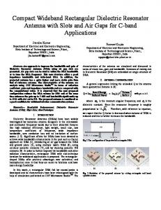
2. Formulation 2.1. Fields in Cartesian coordinates For electromagnetic waves propagating in the z direction of a rectangular waveguide, as shown in Fig. 1, Helmholtz equations are expressed in Cartesian coordinates as [35–37] 2

2

∂ ψz ∂ ψz ---------------- + ---------------- + ( k 2 – k z2 ) ψ z = 0 2 2 ∂x ∂y

(1)

where ψz is the z component of a two dimensional vector phasor ψ that depends on the cross-sectional coordinates. To derive the field components in the waveguide, ψz can be substituted with the longitudinal electric Ez and magnetic Hz fields.

Propagation in dielectric rectangular waveguides

319

b y z 0

a

x

Fig. 1. Dielectric rectangular waveguide.

The transverse field components are obtained by substituting Ez and Hz into Maxwell’s source free curl equations. Rearranging the transverse fields by expressing them in terms of the longitudinal fields, we obtain the following: dH z dE z  –j -  k z -------------- – ω ε ------------H x = --------------------2 2  dx dy  kx + ky

(2)

dH z dE z  –j -  k -------------- – ω ε ------------H y = --------------------2 2  z dy dx  kx + ky

(3)

dE z dH z  –j -  k z ------------- – ω μ -------------E x = --------------------2 2  dx dy  kx + ky

(4)

dE z dH z  –j -  k ------------- – ω μ -------------E y = --------------------2 2  z dy dx  kx + ky

(5)

where ε and μ are the permittivity and permeability of the inner core material, respectively. For a non-magnetic material, μ is identical with the permeability of free space μ 0. Generally, the permittivity ε of a lossy material is complex and is given as [34, 38]

σ ε = ε 0 – j -------(6) ω where ε 0 and σ are respectively the permittivity and conductivity of the material, and ω is the angular frequency. However, since the conductivity of the dielectric material is almost negligible, the imaginary part in (6) can be neglected and ε in the inner core

is usually taken as a real value. The permittivity at the wall, on the other hand, could be either complex (for conductor) or real (for dielectric), depending on the cladding material at the wall. 2.2. Fields in a dielectric rectangular waveguide In general, the dielectric constant of a dielectric waveguide is higher than its surrounding medium, which, in most cases, is the air. This allows the fields to be confined most-

320

KIM HO YEAP et al.

ly within the waveguide and decays in evanescence beyond the boundary of the waveguide. Since the fields are concentrated at the core of the waveguide, the resultant tangential electric field Et and the normal derivative of the tangential magnetic field ∂Ht /∂an are at their minimal (but not necessarily zero) at the boundary of the waveguide. Using the method of separation of variables to solve (1), the longitudinal fields can be expressed as: E z = E 0 sin ( k x x + φ x ) sin ( k y y + φ y )

(7)

H z = H 0 cos ( k x x + φ x ) cos ( k y y + φ y )

(8)

where E0 and H0 are the constant amplitudes of the fields. The phase parameters φ x and φ y , are referred to as the field’s penetration factors in the x and y directions, respectively [34]. The penetration factors account for the remaining fields at the boundary, which decays exponentially beyond the boundary. Since both Et and ∂Ht /∂an are either at their maximum or zero at the centre of the waveguide, i.e., ky b kx a sin ------------ + φ x = sin ------------ + φ y = ± 1 or 0  2   2 

(9)

where a and b are the width and height of the waveguide, respectively, then, the penetration factors can be found as: pπ – k a

x φ x = --------------------------

(10)

2

qπ – k y b

φ y = ---------------------------

(11)

2

y

x

In order to account for the coexistence of E pq and E pq modes, both longitudinal fields must be present. Hence, substituting the longitudinal fields (7) and (8) into (2) to (5), the transverse fields are obtained as: j ( k z k x H 0 + ω ε d k y E 0 ) sin ( k x x + φ x ) sin ( k y y + φ y ) H x = ----------------------------------------------------------------------------------------------------------------------------------2 2 kx + ky

(12)

j ( k z k y H 0 + ω ε d k y E 0 ) cos ( k x x + φ x ) sin ( k y y + φ y ) H y = -----------------------------------------------------------------------------------------------------------------------------------2 2 kx + ky

(13)

j ( k z k x E 0 + ω μ d k y H 0 ) cos ( k x x + φ x ) sin ( k y y + φ y ) E x = ------------------------------------------------------------------------------------------------------------------------------------2 2 kx + ky

(14)


j ( k z k y E 0 + ω μ d k x H 0 ) sin ( k x x + φ x ) cos ( k y y + φ y ) E y = -----------------------------------------------------------------------------------------------------------------------------------2 2 kx + ky

321

(15)

where ε d and μ d are the permittivity and permeability of the dielectric material, respectively. 2.3. Constitutive relations At the boundary of the dielectric waveguide, the ratio of the tangential electric field Et to tangential magnetic field Ht is related to the surface impedance Zs as [34–36] Et ---------------------- = Zs an × Ht

(16)

where an is a normal unit vector; Zs can be expressed in terms of the electrical properties of the two mediums [39] 1 Z s = ---------------------------------------jω ( ε rd – ε r0 )b

(17)

where ω is the angular frequency, whereas ε rd and ε r0 are the relative permittivities of the waveguide and the surrounding material, respectively. For simplicity, we are considering a single layer dielectric waveguide surrounded by air. At the height surface of the waveguide where y = b, Ez /Hx = –Ex /Hz = Zs. Substituting (7), (8), (12), (14) and (17) into (16), the following relationships are obtained: E0 –Ex j 1 ------------- = --------------------- --------- k z k x – ω μ d k y tan ( k y b + φ y ) = ---------------------------------------- (18a) 2 2  H  ω ( ε Hz j rd – ε r0 )b 0 kx + ky H0 Hx j --------- = --------------------- ---------- k k + ω ε d k y cot ( k y b + φ y ) = jω ( ε r – ε r )b d 0 2 2  E0 z x  Ez kx + ky

(18b)

Similarly, at the width surface of the waveguide where x = a, Ey /Hz = –Ez /Hy = Zs. Substituting (7), (8), (13), (15) and (17) into (16), the following relationships are obtained: Ey E0 –j 1 ---------- = --------------------- --------- k z k y + ω μ d k x tan ( k x a + φ x ) = ---------------------------------------2 2   Hz jω ( ε rd – ε r0 )b kx + ky H0

(19a)

–Hy H0 –j -------------- = --------------------- ---------- k z k y – ω ε d k x cot ( k x a + φ x ) = jω ( ε r – ε r )b d 0 2 2   Ez kx + ky E0

(19b)

322

KIM HO YEAP et al.

In order to obtain non-trivial solutions for (18) and (19), the determinants of the equations must vanish. This leads us to the following set of transcendental equations jω μ 0 k y tan ( k y b + φ y ) 1 -------------------------------------------------------- + ---------------------------------------- × 2 2 jω ( ε rd – ε r0 )b kx + ky jω ε 0 k y cot ( k y b + φ y ) × ------------------------------------------------------– jω ( ε rd – ε r0 )b 2 2 kx + ky

 k z k x 2 - =  ------------------- k x2 + k y2 

(20a)

 k z k y 2 - =  ------------------- k x2 + k y2 

(20b)

jω μ 0 k x tan ( k x a + φ x ) 1 -------------------------------------------------------- + ---------------------------------------- × 2 2 jω ( ε rd – ε r0 )b kx + ky jω ε 0 k x cot ( k x a + φ x ) × ------------------------------------------------------– jω ( ε rd – ε r0 )b 2 2 kx + ky

In (20), the transverse wave numbers kx and ky are the complex variables to be solved for. A root-searching algorithm can be used to find the roots of kx and ky. The solutions of kx and ky are then substituted into the dispersion relation which relates the transverse wave numbers with the propagation coefficient kz: kz =

2

2

2

k – kx – ky

(21)

Here, the propagation coefficient kz is a complex variable which is denoted as kz = = β z – jα z, where β z is the phase coefficient and α z – the attenuation coefficient of the waves. Hence, by extracting the real and imaginary values from kz, both the phase and attenuation coefficients could be obtained.

3. Results and discussion To validate our formulation, we compute the propagation coefficient kz of waves traveling in a WR10 silicon waveguide with size 2.4×1.3 mm2. Since Marcatili’s formulation has popularly been used in the design of dielectric rectangular waveguides [1–3], we compare our results with those obtained from Marcatili’s approach and the finite element method (FEM). The results from the FEM are simulated from Ansoft’s high frequency structure simulator (HFSS). Unlike a hollow conducting rectangular wavey guide in which TE10 is known to be the fundamental mode, Marcatili has suggested E 11 x and E 11 to be the fundamental modes in a dielectric rectangular waveguide [19, 20]. In his analysis, however, none has been discussed on the condition when pq = 10. WELLS has simulated the fields’ distribution in a dielectric rectangular waveguide [2]. It is shown in the results that some of the field patterns resemble closely that of the TE10 mode, i.e., the cross-section exhibits half-wave field variation in the x-direction;


323

Attenuation [Np/m]

2000

1500

1000

500

0 2.5

7.5

12.5

17.5

22.5

27.5

32.5

Frequency [GHz] y

y

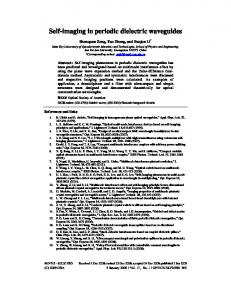
Fig. 2. Attenuation of E 10 (dashed line) and E 11 (dashed-dotted-dotted line) in a dielectric rectangular waveguide.

but almost uniform field distribution in the y-direction. WELLS’ result indicates that mode 10 could have existed in a dielectric rectangular waveguide. However, it is not certain if there is a switch in the fundamental mode from 10 to 11. Here, to further analyze both modes, we have computed and compared the attenuation coefficient for both pq = 10 and 11 modes using Marcatili’s transcendental equations. Since it is revealed in WELLS’ paper [2] that when a shield is coated at the wall of the waveguide, y y E 11 changes to TE10, we have applied the equations which describe E pq in our calcuy y lation. As can be seen in Fig. 2, E 10 has a lower cutoff frequency fc than that of E 11 . This is to say that, notwithstanding the material used for the wall, pq = 10 remains unchanged as the first mode to propagate in a rectangular waveguide. Indeed, such phenomenon is to be expected. Since it has been found that the first mode in a circular dielectric waveguide remains similar to that of its hollow conducting counterpart [40], naturally, this phenomenon should not have changed for the case of a rectangular waveguide as well. y Figures 3 and 4 depict the attenuation of E 10 in the dielectric rectangular waveguide. As can be clearly seen in Fig. 3, the attenuation predicted by both Marcatili’s transcendental method and our method agrees very well with HFSS simulation result at frequencies at the vicinity of cutoff fc. As shown in both Figs. 3 and 4, the attenuation and the cutoff frequency fc predicted by Marcatili’s closed form equation are somewhat lower than the simulation results. Since the closed form equation is a simplification of its transcendental form, the significant discrepancies found using this approximate method should be of no surprise at all and can be attributed to the assumptions made to simplify the formulation. After close inspection on the attenuation above fc, it could be observed from Fig. 4 that the attenuation computed using our method agrees very well with the simulation results and is, in fact, almost indistinguishable with each other; Marcatili’s transcendental method, on the other hand, has overestimated the attenuation exhibited in the dielectric waveguide. Hence, it is sufficient to say that although Marcatili’s transcendental equation shows high accuracy below cutoff fc, it fails to give accurate loss prediction for waves propagating above fc. One reason why our result is

324

KIM HO YEAP et al.

Attenuation [Np/m]

1180

780

380

–20 2.5

7.5

12.5

17.5

Frequency [GHz] y

Fig. 3. Attenuation of E 10 below cutoff, computed using Marcatili’s closed form equations (dashed -dotted-dotted line), Marcatili’s transcendental equations (dashed line), our method (solid line), and HFSS simulation (dashed-dotted line).

Attenuation [Np/m]

19.5

14.5

9.5

4.5

–0.5 18.2

18.3

18.4

18.5

18.6

Frequency [GHz] y

Fig. 4. Attenuation of E 10 above cutoff, computed using Marcatili’s closed form equations (dashed -dotted-dotted line), Marcatili’s transcendental equations (dashed line), our method (solid line), and HFSS simulation (dashed-dotted line).

found to be in close agreement with the simulation result is that our method has not only considered the interaction of fields at the boundary of the width and height surfaces, but also those at the four edges of the rectangular waveguide. By including the analysis of fields at the edges, allowing the penetration of fields at the wall of the waveguide, as well as accounting for the superposition of modes, our method actually gives a more realistic behaviour of the propagation of fields in the dielectric rectangular waveguide. Despite being popularly implemented in the millimeter and submillimeter circuits, we found that data and analysis which compare the performance of both dielectric and metallic waveguides are surprisingly rare in the literature. Here, we investigate the attenuation in three different kinds of rectangular waveguides, i.e., a silicon waveguide, a hollow copper waveguide and a silicon waveguide coated with a copper wall. The size


325

of both silicon waveguides remains as 2.4×1.3 mm2. Since the cutoff frequency fc of a waveguide is dependent on the constitutive properties of the dielectric medium, as follows [41, 42]: pπ 2 qπ 2 1 f c = -------------------------------- ------------ + ------------  a   b  2π μ d ε d

(22)

we have adjusted the size of the hollow conducting waveguide so as to give the same cutoff frequency fc as the other two waveguides. The size of the hollow waveguide is given as 8.28×4.49 mm2. The attenuation in the silicon waveguide is computed using (20) and (21). The attenuations in both the hollow copper waveguide and the silicon waveguide with the copper wall, on the other hand, are computed based on the equations in [34]. For convenience, we outline the transcendental equations for computing the transverse wave numbers kx and ky in [34] as follows: jω μ 0 k y tan ( k y b + φ y ) -------------------------------------------------------- + 2 2 kx + ky

μ

0 --------------------------σc ε c – j ----------

ω

jω ε 0 k y cot ( k y b + φ y ) × ------------------------------------------------------– 2 2 kx + ky jω μ 0 k x tan ( k x a + φ x ) -------------------------------------------------------- + 2 2 kx + ky

×

σc ε c – j ---------ω ---------------------------μ0

μ

0 --------------------------σc ε c – j ----------

jω ε 0 k x cot ( k x a + φ x ) × ------------------------------------------------------– 2 2 kx + ky

 k z kx 2 - =  ------------------- k x2 + k y2 

(23a)

 k z ky 2 - =  ------------------- k x2 + k y2 

(23b)

×

ω

σc ε c – j ---------ω ---------------------------μ0

where εc and σc are respectively the permittivity and conductivity of the copper wall. Like the case of the dielectric waveguide in this paper, the transverse wave numbers are first numerically solved. The solutions are then substituted into (21) to obtain the attenuation constant of the metallic waveguides. Figure 5 depicts the attenuation of the dominant mode in the waveguides at frequency f below cutoff fc, while Figs. 6 and 7 illustrate the attenuation beyond cutoff. As can be observed in Fig. 5, at f below fc, the loss in the two silicon waveguides is comparable to each other. At f above fc, however, Figs. 6 and 7 show that the silicon

326

KIM HO YEAP et al.

Attenuation [Np/m]

1180

780

380

–20 2.5

7.5

12.5

17.5

Frequency [GHz]

Fig. 5. Attenuation of the dominant mode below cutoff, in a silicon rectangular waveguide (solid line), silicon rectangular waveguide with copper wall (dashed-dotted line), and hollow copper rectangular waveguide (dashed line).

Attenuation [Np/m]

5 4 3 2 1 0 18.35

18.45

18.55

18.65

Frequency [GHz]

Fig. 6. Attenuation of the dominant mode immediately after cutoff, in a silicon rectangular waveguide (solid line), silicon rectangular waveguide with copper wall (dashed-dotted line), and hollow copper rectangular waveguide (dashed line).

Attenuation [Np/m]

1.6 1.2 0.8 0.4 0.0 20

21

22

23

Frequency [GHz]

Fig. 7. Attenuation of the dominant mode above cutoff, in a silicon rectangular waveguide (solid line), silicon rectangular waveguide with copper wall (dashed-dotted line), and hollow copper rectangular waveguide (dashed line).


327

waveguide surrounded with the copper wall exhibits considerably higher loss. Since wave propagation is generally confined within the waveguides, radiation loss is practically negligible in both types of waveguides. Hence, the two main factors which contribute to the loss in a waveguide are the dielectric and conduction losses [41]. The loss in the metallic waveguide is found to be higher mainly because, besides having dielectric loss at the silicon core, it also experiences conduction loss at the copper wall. With the absence of the outer conducting wall, the dielectric silicon waveguide, on the other hand, only experiences dielectric loss. This study confirms the notion that dielectric waveguides are generally believed to have lower loss, compared to their metallic counterparts [1–3]. It is worthwhile noting, however, that there is one exceptional case in which the loss in a metallic waveguide could be significantly lower than dielectric waveguides. As shown in Figs. 5 to 7, the loss in the hollow conducting copper waveguide is considerably lower than that in the dielectric silicon waveguide. This is because air has generally much lower dielectric loss than any other kind of dielectric materials. The low loss found in hollow waveguides is also the reason why hollow conducting waveguides are widely used in radio receiver systems built particularly to detect the extremely weak extraterrestrial signals at millimeter and submillimeter wavelengths [43–46]. However, it could also be seen here that while hollow waveguides exhibit much lower attenuation, they come at the expense of size. For waveguides which allow signals with the same cutoff frequencies to propagate, the size of the hollow waveguide is usually larger. After close inspection on (22), we can find that the size of the hollow waveguide is about ε r1/2 times larger than its dielectric counterd part. It is also worthwhile noting that the fabrication cost for hollow conducting waveguides is usually higher than dielectric waveguides as well. This is partly due to the highly conducting material which is more expensive than dielectric; and partly also, because the process involved in the fabrication of metallic waveguides is usually more laborious. Unlike dielectric waveguides which generally require only the technique of lithography, etching and dielectric deposition, fabricating metallic waveguides may require the additional step of electroforming the conducting layer onto the dielectric core. Electroforming is an electrodeposition process which involves immersing the waveguide (which is solely dielectric at this stage) into a conducting electrolyte so as to allow metallic ions to build up at the outer layer, forming a metallic coating at the waveguide. This additional step will certainly contribute to the cost in fabricating metallic waveguides.

4. Conclusion A fundamental and accurate technique to compute the propagation constant of waves in a dielectric rectangular waveguide is proposed. The formulation is based on matching the fields to the constitutive properties of the material at the boundary. At the waveguide wall the surface current density divided by the tangential electric field is matched with the surface impedance of the wall. Doing so, we obtain two sets of equations which describe the surface impedance at the width surface and another two sets at the height

328

KIM HO YEAP et al.

surface. The equations admit non-trivial solutions only when their determinants are zero. The expansion of the determinants lead to transcendental equations, whose roots are the allowed values for the transverse wave numbers in the x and y directions, i.e., kx and ky , respectively, for different modes. The wave propagation constant kz could be found by relating kx, ky , and kz using the dispersion relation. The attenuation curves obtained are in good agreement with those obtained from the finite element method (FEM). An important implication of this work is that the fundamental mode is observed to be pq = 10. It is also observed that hollow conducting waveguides exhibit much lower attenuation than dielectric waveguides. This can be explained by the low dielectric loss in free space, compared to other dielectric materials. Although more superior in preserving the energy of the waves, for a signal with the same fc to propagate, the hollow waveguide is generally much larger in size compared to its dielectric counterparts. Acknowledgements – Part of this work has been supported by the Fundamental Research Grant Scheme FRGS funded by the Ministry of Education, Malaysia (project: FRGS/2/2013/SG02/UTAR/02/1).

References [1] HAMILTON D.P., GREEN R.J., LEESON M.S., Simple estimation formulas for rectangular dielectric waveguide single-mode range and propagation constant, Microwave and Optical Technology Letters 49(3), 2007, pp. 503–505. [2] WELLS C.G., Analysis of shielded rectangular dielectric rod waveguide using mode matching, PhD Thesis, University of Southern Queensland, Australia, 2005. [3] DUDOROV S., Rectangular dielectric waveguide and its optimal transition to a metal waveguide, PhD Thesis, Helsinki University of Technology, Finland, 2002. [4] KUZNETSOV M., Expressions for the coupling coefficient of a rectangular-waveguide directional coupler, Optics Letters 8(9), 1983, pp. 499–501. [5] LEUNG K.W., SO K.K., Rectangular waveguide excitation of dielectric resonator antenna, IEEE Transactions on Antennas and Propagation 51(9), 2003, pp. 2477–2481. [6] SALEHI M., BORNEMANN J., MEHRSHAHI E., Wideband substrate-integrated waveguide six-port power divider/combiner, Microwave and Optical Technology Letters 55(), 2013, pp. 2984–2986. [7] LIU J., SAFAVI-NAEINI S., CHOW Y.L., ZHAO H., New method for ultra wide band and high gain rectangular dielectric rod antenna design, Progress in Electromagnetics Research C 36, 2013, pp. 131–143. [8] ENG GEE LIM, ZHAO WANG, JING CHEN WANG, LEACH M., RONG ZHOU, CHI-UN LEI, KA LOK MAN, Wearable textile substrate patch antennas, Engineering Letters 22(2), 2014, pp. 94–101. [9] STRATTON J.A., Electromagnetic Theory, Chapter 9, McGraw-Hill, New York, 1941. [10] COLLIN R.E., Field Theory and Guided Waves, Chapter 5, IEEE Press, New York, 1991. [11] BUCK J.A., Fundamentals of Optical Fibers, Wiley, New York, 2004. [12] YEAP K.H., THAM C.Y., YEONG K.C., WOO H.J., Wave propagation in lossy and superconducting circular waveguides, Radioengineering 19(2), 2010, pp. 320–325. [13] YASSIN G., THAM C.Y., WITHINGTON S., Propagation in lossy and superconducting cylindrical waveguides, [In] Proceedings of the 14th International Symposium on Space Terahertz Technology, Tucson, Arizona, 2003, pp. 516–519. [14] KNOX R.M., TOULIOS P.P., Integrated circuit for millimeter through optical frequency range, [In] Proceedings of the MRI Symposium on Submillimeter Waves, Polytechnic Press, 1970, pp. 497–516.


329

[15] KUMAR A., THYAGARAJAN K., GHATAK A.K., Analysis of rectangular-core dielectric waveguides: an accurate perturbation approach, Optics Letters 8(1), 1983, pp. 63–65. [16] CAI Y., MIZUMOTO T., NAITO Y., Improved perturbation feedback method for the analysis of rectangular dielectric waveguides, Journal of Lightwave Technology 9(10), 1991, pp. 1231–1237. [17] YOUNG P.R., COLLIER J., Solution of lossy dielectric waveguide using dual effective-index method, Electronics Letters 33(21), 1997, pp. 1788–1789. [18] XIA J., MCKNIGHT S.W., VITTORIA C., Propagation losses in dielectric image guides, IEEE Transactions on Microwave Theory and Techniques 36(1), 1988, pp. 155–158. [19] MARCATILI E.A.J., Dielectric rectangular waveguide and directional coupler for integrated optics, The Bell System Technical Journal 48(7), 1969, pp. 2071–2102. [20] CHARLES J., BAUDRAND H., BAJON D., A full-wave analysis of an arbitrarily shaped dielectric waveguide using Green’s scalar identity, IEEE Transactions on Microwave Theory and Techniques 39(6), 1991, pp. 1029–1034. [21] OGUSU K., Numerical analysis of the rectangular dielectric waveguide and its modifications, IEEE Transactions on Microwave Theory and Techniques 25(11), 1977, pp. 874–885. [22] HORN L., LEE C.A., Choice of boundary conditions for rectangular dielectric waveguides using approximate eigenfunctions separable in x and y, Optics Letters 15(7), 1990, pp. 349–350. [23] CHENG Y.H., LIN W.G., Investigation of rectangular dielectric waveguides: an iteratively equivalent index method, IEE Proceedings J – Optoelectronics 137(5), 1990, pp. 323–329. [24] KIM C.M., JUNG B.G., LEE C.W., Analysis of dielectric rectangular waveguide by modified effective -index method, Electronics Letters 22(6), 1986, pp. 296–298. [25] KRAMMER H., Field configurations and propagation constants of modes in hollow rectangular dielectric waveguides, IEEE Journal of Quantum Electronics 12(8), 1976, pp. 505–507. [26] GOELL J.E., A circular-harmonic computer analysis of rectangular dielectric waveguides, The Bell System Technical Journal 48(7), 1969, pp. 2133–2160. [27] RAHMAN B.M.A., DAVIES J.B., Finite-element analysis of optical and microwave waveguide problems, IEEE Transactions on Microwave Theory and Techniques 32(1), 1984, pp. 20–28. [28] VALOR L., ZAPATA J., Efficient finite element analysis of waveguides with lossy inhomogeneous anisotropic materials characterized by arbitrary permittivity and permeability tensors, IEEE Transactions on Microwave Theory and Techniques 43(10), 1995, pp. 2452–2459. [29] SCHWEIG E., BRIDGES W.B., Computer analysis of dielectric waveguides: a finite difference method, IEEE Transactions on Microwave Theory and Techniques 32(5), 1984, pp. 531–541. [30] SOLBACH K., WOLFF I., The electromagnetic fields and the phase constants of dielectric image lines, IEEE Transactions on Microwave Theory and Techniques 26(4), 1978, pp. 266–274. [31] EYGES L., GIANINO P., WINTERSTEINER P., Modes of dielectric waveguides of arbitrary cross sectional shape, Journal of the Optical Society of America 69(9), 1979, pp. 1226–1235. [32] MABAYA N., LAGASSE P.E., VANDENBULCKE P., Finite element analysis waveguides of optical, IEEE Transactions on Microwave Theory and Techniques 29(6), 1981, pp. 600–605. [33] ATHANASOULIAS G., UZUNOGLU N.K., An accurate and efficient entire-domain basis Galerkin’s method for the integral equation analysis of integrated rectangular dielectric waveguides, IEEE Transactions on Microwave Theory and Techniques 43(12), 1995, pp. 2794–2804. [34] YEAP K.H., THAM C.Y., YASSIN G., YEONG K.C., Attenuation in rectangular waveguides with finite conductivity walls, Radioengineering 20(2), 2011, pp. 472–478. [35] YEAP K.H., THAM C.Y., YEONG K.C., YEAP K.H., A simple method for calculating attenuation in waveguides, Frequenz – Journal of RF-Engineering and Telecommunications 63(11–12), 2009, pp. 236–240. [36] YEAP K.H., THAM C.Y., YEONG K.C., LIM E.H., Full wave analysis of normal and superconducting microstrip transmission lines, Frequenz – Journal of RF-Engineering and Telecommunications 64(3–4), 2010, pp. 59–66.

330

KIM HO YEAP et al.

[37] BLACKLEDGE J., BABAJANOV B., Three-dimensional simulation of the field patterns generated by an integrated antenna, IAENG International Journal of Applied Mathematics 43(3), 2013, pp. 138–153. [38] WEI B.L., XIONG C., YUE H.W., WEI X.M., XU W.L., ZHOU Q., DUAN J.H., Ultra wideband wireless propagation channel characterizations for biomedical implants, IAENG International Journal of Computer Science 42(), 2015, pp. 41–45. [39] KOLUNDZIJA B.M., OGNJANOVIC J.S., Electromagnetic Modeling of Composite Metallic and Dielectric Structures, Artech House, 2002. [40] BALANIS C.A., Advanced Engineering Electromagnetics, Wiley, New York, 1989. [41] CHENG D.K., Field and Waves Electromagnetics, Addison Wesley, 1989. [42] YEAP K.H., YEONG K.C., CHONG K.H., WOO H.J., RIZMAN Z.I., Plots of field distribution in a rectangular waveguide, International Journal of Electronics, Computer and Communications Technologies 1(2), 2011, pp. 5–13. [43] YEAP K.H., THAM C.Y., NISAR H., LOH S.H., Analysis of probes in a rectangular waveguide, Frequenz – Journal of RF-Engineering and Telecommunications 67(5–6), 2013, pp. 145–154. [44] YEAP K.H., LAW Y.H., RIZMAN Z.I., CHEONG Y.K., ONG C.E., CHONG K.H., Performance analysis of paraboloidal reflector antennas in radio telescopes, International Journal of Electronics, Computer and Communications Technologies 4(1), 2013, pp. 21–25. [45] WITHINGTON S., Terahertz astronomical telescopes and instrumentation, Philosophical Transactions of the Royal Society A: Mathematical, Physical and Engineering Sciences 362(1815), 2004, pp. 395 – 402. [46] PHILLIPS T.G., KEENE J., Submillimeter astronomy, Proceedings of the IEEE 80(11), 1992, pp. 1662 –1678.

Received August 19, 2015 in revised form November 6, 2015