surface is rigid and flat, the upper surface is free. The northern and .... 8=kAx,. CY= ZAy, k is the east-west wave number, and. I is the north-south wave number.
MONTHLY WEATHER REVIEW
606
vel. 99,No. 8 UDC 661.W.313
PROPAGATION OF SYSTEMATIC ERRORS IN A ONE LAYER PRIMITIVE-EQUATION A4 FOR SYNOPTIC SCALE MOTION WILLIAM S. IRVINE, JR,' and DAVID D. HOUGHTON Department of Meteorology, The University of Wisconsin, Madison, Wis.
ABSTRACT A one-layer, mid-latitudeJ beta-plane channel model of an incompressible homogeneous fluid is constructed to study the propagation of systematic errors on a nearly stationary synoptic scale wave. A time- and space-centered difference scheme is used t o evaluate the governing primitive equations. Data fields resulting from height field perturbations injected at various locations in the synoptic wave are compared to the unperturbed synoptic wave at 3-hr intervals for 5 model days. Results show that the low-frequency or quasi-geostrophic component of the error tends to move toward the core of maximum velocity in the basic state and that, after 5 days, these maximum height errors are in the core regardless of the location of the initial perturbation.
1. INTRODUCTION
Recent years have found atmospheric numerical models becoming more sophisticated. Multilayered models, ultrahigh-speed computers, and improved direct observational networks have made accurate global numerical models a reality. One inherent limit to the accuracy of these models, however, is the availability of initializing information. Direct observational data are lacking from large areas of the globe-such as oceans, deserts, the polar regions, and the Tropics. Recent interest has centered on augmentation of existing direct data networks using satellite information. Johnson (1967) and Smith (1967) have proposed schemes to augment available wind and temperature data using satellite photographs and radiation measurements. While this improved data coverage is desirable, preparing these additional data for numerical model use presents some novel problems. Model initialization of single-source data has been investigated by Rossby (1938), Houghton and Washington (1969), and others. This work will investigate one special problem associated with initialization of multiple-source data-that of systematic error propagation. Attention is directed primarily to the low-frequency (synoptic scale) motions, although the high-frequency gravity wave modes are also present. This study has a direct relationship to the problem of predictability. Previous studies by Lorenz (19694 and Smagorinsky (1969) have considered the effect of initial errors or deviations on a forecast in terms of statistical comparisons involving the entire integration domain. I n this study, the comparison is in terms of actual difference maps which can demonstrate the variation in predictability that exists as a function of location. The analysis provides information on the horizontal propagation of information or energy in a simple atmosphere. Knowledge 1
Now &listed with Air Force Global Weather Central, Offutt Air Force Base,Nehr.
of energy propagation in the atmosphere is fundamental to understanding the complicated interactions of atmospheric motions. I n numerical models, there is the additional related problem of error propagation from any artificial boundaries. This study uses a simple one-layer model to perform numerous experiments using variations of one basic initial condition. One-layer modeling has the advantages of economy and simplicity. Shuman (1962), Houghton and Kasahara (1968), and many others have taken advantage of these features to study atmospheric problems as varied as synoptic scale motions and mountain flow. While onelayer models are unrealistic descriptions of certain conditions, such as deep convection and baroclinic development, one may assume that general conclusions can be made applicable to certain modes of multilayer models (and perhaps the real atmosphere). This study will describe a one-layer model and a series of seven experiments involving a typical synoptic scale wave. A synoptic scale wave with negligible east-west trace velocity is run in the model for 5 days. This wave is used as a standard for comparison with six additional experiments. These additional experiments are identical to the first except for a small initial height perturbation located in or near the core of maximum fluid velocity. Conclusions are then made as to the sensitivity of the basic flow to the injection of this small perturbation at six locations. Injecting height perturbations into a basic flow is intended to simulate the incorporation of asynoptic data into a synoptic data network. Here, asynoptic data such as satellite data are expected to exhibit some systematic deviation from conventional data over the entire initial data field. Section 2 describes the model characteristics and the basic equations. In section 3, the stability criteria. (both physical and numerical) are discussed. The initialization procedures are given in section 4, and the numerical experiments are described in section 5 . Finally, experi-
August 1971
William
S. Irvine, Jr., a n d D a v i d D. H o u g h t o n
mental results and conclusions of the study are presented in section 6.
607
These equations can be rewritten in an alternate form to be used for finite differencing as
9. MODEL CHARACTERISTICS
AND BASIC EQUATIONS The model used for this study is a rnid-latitude channel model of an incompressible homogeneous fluid. The lower surface is rigid and flat, the upper surface is free. The northern and southern boundaries are rigid vertical walls and ah a ( h u ) d(hV) where the north-south velocity, V, is constrained to vanish. X + T+ F = O . (6) The flow is made periodic in the east-west direction with a wavelength of 6720 km. The model has the same dimenThe integration scheme used for this model is based on sions and equally spaced grid points in both horizontal directions. The Coriolis parameter is evaluated from a Grammeltvedt’s scheme F (1969). This scheme has the advantage of conserving total momemtum in the nonbeta plane centered at 45’N. linear terms. With his notation, the scheme can be For reducing the speed of gravity wave propagation and written as to simulate motion in the troposphere rather than the entire atmosphere, an inert fluid of infinite depth is placed above (7) the free surface. This effect, described by Houghton et al. (1966), is achieved in actuality by “reducing” gravity in this study from 9.8 t o 1.4 m/sz. The model is initialized by prescribing a stream function. The three dependent variables (height and east-west and north-south fluid velocity) are determined by using balance and quasi-geostrophic divergence relationships, If (Y and @ are general variables, the operators found in discussed further in section 4. Time integration using eq (7-9) can be defined as Grammeltvedt’s scheme F (1969), as formulated in this A=Ax, Ay, At, section, proceeds for 5 days. The model disturbance energy is calculated at each time step to check conservation -2 1 a==- [a($, +A) -a(x*--A)I, of total energy, and the three dependent variables are 2A made available at 3-hr intervals. 1 ZZz=+(x t +A) +&f -4 1 , Symbols used frequently in this work are and Coriolis parameter , reduced acceleration of gravity, depth of the fluid, The finite-difference form of the governing equations all index parameter in the x direction, contain space- or time-centered approximations to the index parameter in the y direction, first derivative terms except a t the northern and southern number of grid points in the x direction, boundaries. Here, because centered space differences in number of grid points in the y direction, the north-south direction are not possible, one-sided time, differences must be used. This noncentered space difference velocity components in the x and y directions, has a noticeable but very small effect on the available east-west and north-south Cartesian coordinates, energy of the model. This was shown by tests using various fluid density (constant), channel shapes. velocity potential, and The total energy of the model, E,can be expressed as the stream function. sum of kinetic and potential energy. Total energy, --” evaluated over the entire volume of the model can be The basic Eulerian equations are expressed as ~ + u - + au v - - - j vau +g a;c=o, ah at
ax
a~
g + uav -+v av -+ at
and
437-755 0
- 71 - 2
ax
ay
f u + g ah -=o,
ay
(2)
for the finite-difference model where
MONTHLY WEATHER REVIEW
608
and subscripts refer to grid position, for example,
U ,j=
u(iA~,jAy).
Total disturbance energy (DE) can be evaluated by subtracting the minimum possible potential energy from the total energy of the system:
vd, 99, No. 8
By writing eq (11-13) in finite differences and assuming periodic solutions of the form U+u" exp(F) with similar expressions for V$jand hTj where
and superscript n refers t*othe time step, space dependence can be eliminated. The resulting equations are
(e@+ +T)
Un+RVn+ 6@hn,
Un+l=U"-I+
or in finite-difference form,
Vn+l=Tm-l -Dun hn+l
where
=hn-1
+(GG+fh')Vn+$TIPl
+8GUn+8TV"+(bG+ @T)h"
(14) (15 )
(IS)
where
a=--
B sin e, T = - J Z B sin CY,
Disturbance energy is a more sensitive indicator of energy changes of the model than the total energy and will be used throughout this paper t o monitor the energy characterisiics of the model.
D= 2 j A f, B=At/Ax, 8=kAx,
3. STABILITY Stability, both computational and physical, is investigated for the model equations and basic flow. Conditions for computational stability may be established by taking the basic model equations in Eulerian form, nondimensionalizing and linearizing t o form
ZAy,
CY=
k is the east-west wave number, and
I is the north-south wave number. Equations (14-16) can be incorporated into a matrix form
(17)
where A is the amplification matrix '
6G
1
a
-D
OG+PT
6T
0
1
86:
6T
i?@+DT
a
1
0
0
1
0 0
0 0 0
0
1
0
0
$G+QT where the transformations made are
o. and
r
c= A
A
A
A
A
gH
where U, V, H , and G are basic characteristic magnitudes for, respectively, the horizontal velocity components, the depth, and the gravity wave propagation speed in the model. Equations (1 1-13), when expressed in a time-space centered finite-difference form, are identical to those resulting from the expansion and linearization of eq (7-9).
D
0 0
The eigenvalues, X, of this amplification matrix are khe roots of the characteristic equation [h(E-A)+1]3=PE2[1+X(L-X)]
(18)
where
L=$G+i?X and
E2=&(@+P)-Lj? There are two sets of unique roots t o this sixth degree
August 1971
William S. Irvine, Jr., and David
609
D. Houghton
1.6 I
20
-
,0
I
1.0
X IC
y
(1000
0.8
kml
FIGURE1.-Zonally
averaged ffuid velocity distribution in the channel for the initial conditions; the abscissa is the distance from the northern boundary.
.6
.4
y
(IOOO km)
FIQURE2.-Values
of absolute vorticity, q, in the channel for the zonally averaged initial fluid velocity; the abscissa is the distance from the northern boundary.
and h=
L& J F 4 . 2
A necessary condition for stability is that the magnitude of all the eigenvalues be less than or equal to one. The conditions established by eq (20) are less restrictive than those of eq (19). There are two possible cases involving the radical in eq (19) : Case I in which (LfE)>,F2that leads to I h l > l for all possible values of e and a. Case I1 in which (LfE ) ,< li-4 that results in 1x151 for all possible values of e and a. Case I1 is of interest since case I will always give unstable conditions, while case I1 will produce, at wonst, neutral stability. Expanding the terms in case 11, one can write
Equation (21) agrees with the results of Richtmyer (1963) for the Lax-Wendroff scheme (1960) in two-space variables. For the parameters of this model, the term A
(1/4)(fAz/Q2 is much less than one and can safely be
ignored. Although computational stability may be assured by a careful choice of At, barotropic instability in the basic flow (as described in sec. 4) is also a possibility. The for this east-west zonal average of the U velocity, flow is shown in figure 1. For a nondivergent one-layer model, a necessary condition for barotropic stability is d$a?J=O (Pedlosky 1964) where is the absolute vorticity defined as
n,
c
For this model,
A
50 m in magnitude) were tracked a t 3-hr intervals as they moved through the basic flow. Time tracks for these selected perturbation blocks are summarized in figures 12-17. The maximum deviation is also plotted for these blocks as a function of time. An estimate of the location, average speed, and maximum magnitude of each block is summarized in table 1 where each perturbation block is identified by a letter-number combination. The letter refers to the experiment, and the number to the order of. appearance in the given experiment. The apparent origin of the block relative to the initial disturbance is determined by extrapolation from the earliest tracked location backward in time to t=O. A dash indicates the lack of a meaningful FIGURE15.-Same as figure 12, except this is for experiment E. numerical value.
1 : 01--O)..
2
6
1
(1000 bm)
50
100
150
200
(597125.2
C E N T E R POINT HAGNlIUDE lm.te,,)
MONTHLY WEATHER REVIEW
614 TABLE1.-Major Perturbation
block
Maximum attained height deviation
(m)
B1 c1
D1 El F1 01
B2 C2
D2 E2 F2 02
perturbation disturbance blocks Time, to, when height dis placement first exceeds 50 m
0
+489
+362
0 0
+623
0
36 21
-87
46
-6.5
Ill5
B4 E4
@Is)
-
21 24
1
Apparent origin measured east ward from initial perturbation location
0
-
0
8 10 7
1320 1320 1440 1320 1440
0 0
0 0
9
8
-
+m
36 36 63 48
+141 +110
105
-
-102 152
72 99
-
2640 2880
9
8
66
-
vol. 99,No. 8
,
(W
0 0
-125 -180 -116 -145
+197 +232 +I85
Eastward velocity
(hr)
+479 +489 $597
B3 c3 D3 E3 F3 03
1.0
6
-
9
3120
8
2880
6 6
-
I
30
60
TIME
90
17.0
(hours)
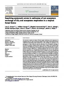
FIGURE lg.-Smoothed and normalized rms values for the height deviations in experiments B through G .
-
also shown in figure 18. The rms values were also normalized, filtered, and hand-smoothed for each experiment B through G. Figure 19 shows the resultant curves. Disturbance energy was calculated for each experiment a t each time step. Although very small fluctuations of disturbance energy could be seen (perhaps due to boundary effects), the total disturbance energy did not fluctuate by more than 0.1 percent for any experiment. 6. EXPERIMENTAL RESULTS AND CONCLUSIONS
30
TIME
60
PO
120
thourr)
FIGURE 18.-Filtered rms values for the height deviations (dashed lines) and maximum perturbation center-point magnitude (solid lines) a t 3-hr intervals for experiment C.
The height deviation fields were analyzed by calculating the root mean square (rms) values (after Lorenz 196%) at 3-hr intervals for each experiment. When one uses the same notation as before, the rms value for experiments B through G at time t i s
The resulting time series of rms values were smoothed by a low-pass filter and are presented for experiment C in figure 18. For comparison with these rms values, the absolute value of the maximum height perturbation is
The height deviation fields (discussed in sec. 5) when viewed sequentially for each experiment have many similar features. Table 1 shows the location and duration of the principal perturbation blocks. During all experiments, the initial unbalanced height perturbation rapidly approaches balance with the fluid velocity field. During this process of about 6-hr duration, the center point magnitude decreases from about 500 to 100 m. This time factor depends on the horizontal space scale of the initial perturbation which is the same in all experiments in this study. This initial perturbation remains quasi-stationary and exhibits only a slight tendency to move with the main fluid flow. After the initial adjustment period, the center point magnitude slowly decreases until, after about 60 hr, the initial block is no longer discernible except in experiment G. This is consistent with elementary adjustment theory which predicts that the height field adjusts to the velocity field for a perturbation with a horizontal length scale less than the A radius of deformation (defined Clf) which is the case here. After 2 1 4 5 hr, a second negative perturbation block appears downstream from the initial disturbance. I n experiment G, this occurs much later. While growing rapidly, this block moves eastward at an average velocity of 8 m/s or about one-quarter of the maximum fluid velocity. This perturbation also begins to weaken after a time and even disappears after 5 days in three of the
Augusf 1971
'
William
S.
Irvine, Jr., a n d D a v i d
experiments. If the motion of each of these perturbations is extrapolated backward in time to t=O.O hr, this second perturbation originates a t an apparent origin about 13001400 km east of the initial perturbation. The third perturbation in all experiments is a positive one and first appears at 36-66 hr except much later in experiment G. This perturbation grows rapidly to f200 m or more and appears to have stopped growing when the model is terminated at 120 hr. This third block also moves eastward with a velocity of about 8 m/s. The apparent origin for the third block is generally from 2600-2700 km east of the initial perturbation for all experiments. A fourth negative block appears in experiments B and E but does not appear in the others. The fourth block has the same general characteristics as the preceding blocks. There are a few significant differences in the motion of all blocks for all experiments. There appear t o be two types of response. Examining the initial appearance time, to, for the second and third blocks, one can contrast experiments B, C, and E with those of D, F, and G. There appears t o be a 12-hr delay in the appearance of D2 as compared. to B2, C2, and E2. This delay is longer for block F2 and longest for block G2. Similar conclusions hold for the third blocks. A second differentiating characteristic is the maximum value of each perturbation. Again, the maximum values of B, C, and E are larger than D, F, and G for blocks 2 and 3. Block 1 is not considered since this information was specified initially. It appears from the above results that experiments B, C, and E have many similar characteristics, as do D, F, and G. It should be re-emphasized that perturbation blocks in experiments B, C, and E were located initially in the main fluid velocity core. The perturbation blocks in experiments D and F were only partially in this core while in G the initial perturbation block was entirely outside the core. The smoothed, normalized rms values for each experiment (fig 19) give additional support t o this distinction. Again, rms values for B, C, and E are larger than D, F, and G after 45 hr. One can easily be misled by these rms values, however, as can be seen from figure 18. The rms plot for experiment C is increasing slowly in time. A better picture of this growth can be seen from the dashed curve (maximum center point magnitude). Here, it is obvious that the maximum perturbation value more than doubles during the final 110 model hours while the rms value only increases by 50 percent during this same time period. The other four perturbation experiments showed similar results. The rms curve is thus a very conservative measure of the increase in magnitude of these traveling disturbances. The second curve in figure 18-maximum perturbation value-perhaps would be a better estimate of this growth. The north-south motion of the perturbation blocks, while not analyzed in detail, shows uniform results. Traveling perturbation blocks tended to follow the northsouth motion of the maximum fluid velocity core. I n the experiments with the initial perturbation field located to 431-755 0
- 71 - 3
D. H o u g h t o n
61 5
one side of the fluid velocity core, the response indicated a gradual migration of this perturbation toward the jet core. The initial perturbation, quasi-stationary in nature, tended t o be most persistant north of the synoptic trough and south of the ridge, especially in experiments D, F, and G. I n experiment G, the initial perturbation remains as a nearly isolated anticyclonic gyre for the entire forecast period. The traveling perturbations covered at least as much area in the horizontal plane as did the initial perturbation. The broadest (and most diffuse) perturbations developed in the initial perturbation in experiments D, F, and G after 20 model hours. Thus, one can see that these perturbations or systematic errors superimposed on a stationary wave can, over a period of 5 days, lead to large traveling disturbances. The closer these disturbances are to the maximum fluid velocity core, the faster they grow. Perturbations injected into the flow, away from the main core, will also form traveling disturbances. However, in this case, they take an appreciably longer time to evolve. The most significant errors that develop away from the initial source region are always in or very near the jet stream axis. Care must be taken when initializing multiple-source data to a numerical model to reduce or at least monitor the effects of these systematic errors as they travel downstream at about 50 percent of the average fluid velocity. The initial error results in high-frequency gravity waves and low-frequency quasi-geostrophic motions. Results of this study suggest that the latitudinal propagation of the low-frequency error fields is remarkably limited in the absence of fluid advection. This would be expected for Rossby wave motions of small scale in the absence of other wave motions. The interaction between the lowfrequency error field and the large-scale motions is primarily limited to advection affects caused by the largescale motions; however, other significant interactions are present. The high-frequency gravity wave motions have minimal interaction with the synoptic scale motions and can be properly sorted out by considering the time-averaged final computed solutions. As a suggestion for further research, it would be valuable at this point to generalize these results t o study the vertical propagation of these disturbances in a multilayer model. I n such a model, one would expect a more continuous spectrum of motions in frequency space especially associated with error perturbations; and the resultant interactions with the basic synoptic scale flow could be far more intricate. Also desirable is the development of techniques for matching the direct and indirect data from multiple sources to reduce these systematic disturbances. ACKNOWLEDGMENTS The authors wish t o thank Prof. John A. Young for his comments on the research presented here. This research was supported by the Atmospheric Sciences Section, National Science Foundation Grant GA-12112.
MONTHLY WEATHER REVIEW
616 REFERENCES
Vel, 99, No. 8
Pedlosky, Joseph, “The Stability of Currents in the Atmosphere and the Ocean: Part I,” Journal of the Atmospheric Sciences, Vol. 21, Grammeltvedt, Arne, “A Survey of Finite-Difference Schemes for No. 2, Mar. 1964,pp. 201-219. the Primitive Equations for a Barotropic Fluid,” Monthly Weather Phillips, Norman A., “On the Problem of Initial Data for the Review, Vol. 97, No. 5, May 1969,pp. 384-404. Primitive Equations,” Tellus, Vol. 12, No. 2, Stockholm, Sweden, Houghton, David D., and Kasahara, Akira, “Non-Linear Shallow May 1960, pp. 121-126. Fluid Flow Over an Isolated Ridge,” Communications on Pure and Richtmyer, Robert D., “A Survey of Difference Methods for NonApplied Mathematics, Vol. 21, No. 1, Jan. 1968,pp. 1-23. Steady Fluid Dynamics,” NCAR Technical Noted 63-2, National Houghton, David D., Kasahara, Akira, and Washington, Warren Center for Atmospheric Research, Boulder, Colo., 1963, 25 pp. M., “Long-Term Integration of the Barotropic Equations by the Rossby, Carl Gustav, “On the Mutual Adjustment of Pressure and Lax-Wendroff Method,” Monthly Weather Review, Vol. 94, No. 3, Velocity Distributions in Certain Simple Current Systems, 11,” Mar. 1966, pp. 141-150. Journal of Marine Research, Vol. 1, No. 3, Sept. 20, 1938, pp. 239Houghton, David, and Washington, Warren M., “On Global 263. Initialization of the Primitive Equations: Part I,” Journal of Shuman, Frederick G., “Numerical Experiments With the Primitive Applied Meteorology, Vol. 8, No. 5, Oct. 1969, pp. 726-737. Equations,” Proceedings of the International Symposium 0% NUJohnson, Michael H., “A Photogrammetric Technique for Finding merical Weather Prediction, Tokyo, Japan November 7-13, 1960, Winds From Satellite Photos,” Studies in Atmospheric Energetics Meteorological Society of Japan, Tokyo, Mar. 1962, pp. 85-107. Based on Aerospace Probings, Annual Report, Contract No. W B G Smagorinsky, Joseph, “Problems and Promises of Deterministic 27, Department of Meteorology, The University of Wisconsin, Extended Range Forecasting,” Bulletin of the American MeteoroMadison, 1967,231 pp. (see pp. 1-18). logical Society, Vol. 50, No. 5, May 1969,pp. 286-312. Lax, Peter D., and Wendroff, Burton, “Systems of Conservation Smith, William L., “An Iterative Method for Deducing Tropospheric Laws,” Communications on Pure and Applied Mathematics, Vol. 13, Temperature and Moisture Profiles From Satellite Radiation Interscience Publications, Inc., New York, N.Y., 1960,pp. 217Measurements,” Monthly Weather Review, Vol. 95, No. 6, June 237. 1967, pp. 363-369. Lorenz, Edward N., “Atmospheric Predictability as Revealed by Stephens, J. J., “Variational Initialization With the Balance EquaNaturally Occurring Analogues,” Journal of the Atmospheric tion,” Journal of Applied Meteorology, Vol. 9, No. 5, Oct. B m , Sciences, Vol. 26, No. 4, July 1969~1, pp. 636-646. pp. 732-739. Lorenz, Edward N., “The Predictability of a Flow Which Possesses Wiin-Nielsen, A., “On Short- and Long-Term Variations in QuasiBarotropic Flow,” Monthly Feather Review, Vol. 89, No. 11, NOV. Many Scales of Motion,” Tellus, Vol. 21, No. 3, Stockholm, 1961,pp. 461-476. Sweden, Aug. B969b,pp. 289-307.
[Received July $1, 1970; revised November 16, 19701