Propagation of variances of FRFs through FRF-based coupling calculations R. Iankov, D. Moens, P. Sas KULeuven, Department of Mechanical Engineering, Celestijnenlaan 300 B, B-3001, Heverlee, Belgium e-mail:
[email protected]
L. Hermans LMS International, CAE Division, Interleuvenlaan 68, B-3001, Leuven, Belgium e-mail:
[email protected]
Abstract In many engineering cases, uncertainties will exist on the frequency response functions (FRFs) of component models. Possible sources of uncertainty in the mechanical structure are uncertain material properties, loading conditions or geometry. When bringing together the component models together and interconnecting them into an assembly, it is of high interest to be able to predict the uncertainty of the response of the assembled system. This paper outlines a technique allowing such an uncertainty characterization. The underlying idea of the approach is based on variance propagation through FRF-based coupling techniques. An analytical approximation using a mean value first order second moment approach (MV) is proposed, which significantly reduces the computational cost involved in a probabilistic uncertainty quantification through the common Monte Carlo (MC) simulation technique. A two-component carbody-subframe assembly model indicates that the overall efficiency of the analytical approach is superior to the classical Monte Carlo simulation approach, while the accuracy obtained with both approaches is very similar.
1
Introduction
The Frequency Based Substructuring (FBS) technique is a tool to predict the dynamic behavior of a coupled system on the basis of the free-interface FRFs of the uncoupled components [1,2]. It allows predicting the global frequency response function matrix between forces acting at specific operational excitation DOFs on a substructure and selected response DOFs in any substructure of the assembly. No limitations are set on the type of response signals: sound pressure, vibrations or reaction forces are treated in a similar way. FBS has been used in vibro-acoustic engineering for several years to predict the dynamic response of coupled systems using FRF data of each substructure, obtained either experimentally or numerically [3,4]. From a component designer’s point of view, the FBS substructuring technique is very attractive as it easily allows producing the force transmissibilities between the input points and the coupling points. Using these force transmissibilities, the reaction forces at the coupling DOFs can be easily derived. These forces can then be applied to the original, uncoupled FE or test component model for design optimization. As the FBS method directly works with compact FRF representations of each component, it is also of
particular interest for hybrid coupling, whereby the low modal density component is represented by FE data and the other component (typically having a high modal density) is represented by test data. Compared to the modal or CMS coupling approach, the FRF nature of the method offers the advantage having the ability to predict the vibro-acoustic response in the medium frequency range, where providing modal basis for each component becomes impractical [5]. The principle of the FBS substructuring procedure consists of dividing a model into two (or more) component models, so-called substructures. Each component model is represented by its FRF matrix [H]. This matrix describes the frequency dependent interaction between force input DOFs, the response DOFs and the coupling DOFs connecting the component to other components. The FRF matrix of each component is either directly measured or synthesized based on a FE or modal model of the component. The FRFs of the assembled structure C are derived starting from the compatibility conditions for the displacements at the interface DOFs as well as the equilibrium conditions of the interface forces. This leads to the following general coupling formula [1]:
1845
1846
P ROCEEDINGS OF ISMA2002 - VOLUME IV
(
)
−1 H − H [ H ]SS + [ B H ]SS + [K ]−SS1 { A H }Sj A ij A iS A if i , j ∈ A H − H [ H ] + [ H ] + [K ]−1 −1 { H } B ij B A B SS B iS SS SS Sj C H ij = if i , j ∈ B −1 −1 − A H iS [ A H ]SS + [ B H ]SS + [K ]SS {B H }Sj if i ∈ A, j ∈ B
(
)
(
(1)
)
In this equation, the uncoupled substructures are referred to as component A and B and the coupled system is denoted by C. Further, S is the subscript for the coupling DOFs between components A and B. A H ij , B H ij and C H ij are the FRFs respectively on A, B and C between nodes i and j. A H iS and B H iS represent rows of the FRFs between node i of component A respectively B and the interface DOFs S. { A H }Sj and { B H }Sj represent columns of the FRFs between all interface DOFs S and reference DOFs j of component A respectively component B. The joint stiffness matrix [K ]SS equals:
[K ]SS
k1 + jωd1 0 = Μ 0
0
Λ
k 2 + jωd 2
Λ
Μ
Ο
0
Λ
0 Μ k s + jωd s 0
−1
(2)
with k i the spring and d i the damping coefficients of the i-th coupling DOF of the flexible joint. The quality of predictions made with this technique is dependent on the inversion of the −1 kernel matrix [H ]SS = [A H ]SS + [B H ]SS + [K ]SS . In the case of rigid coupling, the stiffness matrix [K ]SS does not appear in the kernel, and the individual structural matrix will dominate the quality of the inversion. In the case of flexible joints, the inversion may be less problematic, due to the fact that the coupling flexibility can enhance the condition number of the matrix. In many cases, uncertainties will exist on the FRF representation of each component model. Possible sources of uncertainty in the mechanical structure are uncertain material properties, loading conditions or geometry. When measured data are used, also human error and the calibration tolerance are sources of uncertainty. All of these could influence the dynamic behavior during the analysis. The uncertainty characterization on component level
can be obtained from test data (e.g. deriving the FRF variance from the coherence function) or from numerical predictions such as probabilistic methods, fuzzy FE, Monte-Carlo simulations, …. . For assembled structures, it is of high interest to know the uncertainty on the FRFs of the coupled system given the uncertainties of each component. This paper describes a computationally efficient approach that allows propagating the component variances through the FBS calculation, resulting in the uncertainty characterization of the assembled system.
2
The variance of the response of the coupled system
2.1 Theoretical background It is assumed that all sources of uncertainty are grouped into a general vector of design variables X = (X1 , X 2 ,K X n ). The variation of these variables may or may not be time dependent. The response of the system is a function of this parameter vector. The proposed approach for the response uncertainty quantification is based on a sensitivity analysis of the system response to uncertainties in the design variables. For this aim a mean value first-order second moment method (MVFOSM or further simply referred to as MV method) is proposed [6, 7]. This method is based on a Taylor series expansion of G (X ) about the nominal or mean value of the design random variables. All components of the uncertain design variable vector are modeled using uncorrelated probabilistic random variables. Let G (X ) denote an input/output frequency response function of the system. A Taylor series expansion of G (X ) about the mean of the design variable vector µ = (µ1 , µ 2 ,K µ n ) gives:
∂G ( X ) i =1 ∂X i n
G( X ) ≈ G ( X ) X =µ + ∑ +
1 n n ∂ 2G(X ) ∑∑ 2 j =1 i =1 ∂X i ∂X j
X =µ
X =µ
(X i − µi )
( X i − µ i )(X j − µ j )
(3)
( )
+ O h2
Taking the expected value of this expression and truncating the series at the linear terms yields the expected value and variance for the response:
U NCERTAINTIES IN STRUCTURAL DYNAMICS AND ACOUSTICS
E [G(X )] ≈ G(X ) X =µ
(4)
∂X k
∂G(X ) ∂X i j=1 i=1 n
n
Var[G(X )] ≈ ∑ ∑
X=µ
n ∂G(X ) Var[G(X )] = σ G2 ≈ ∑ ∂X i i=1
2 σX X =µ 2
i
(6)
with σ 2X the variance of X i . Through this result, the variance of the response result of the analysis can be obtained using the derivatives of the response function to the design variables and the variance of the components of the design variables. This expresses the basic principle of the MV approach. Below, this idea is applied to the FBS equation (1) for both rigid and flexible coupling. i
2.2 Rigid coupling For rigidly coupled systems with node i in component A and node j in component B, the derivatives follow directly from the general substructuring equation for combined structures: H ij = A H iS [H ]SS
−1
{B H }Sj
(7)
∂X k
{B H }Sj
with
∂ [H ]SS ∂X k
(8)
For components of the parameter vector X that belong to the FRF between node i of e.g. component A and the coupling DOFs S, the derivative yields : ∂G(X )
=
∂ A H iS ∂X k
∂ A H iS ∂X k
[H ]SS −1{B H }Sj
(9)
a row vector consisting of all zeros
except for the component corresponding to the kth component in the design variable vector, which equals one. For components of the parameter vector X that belong to the internal FRF between the coupling DOFs S in component A or B (resp. [A H ]SS and [B H ]SS ), the derivative yields:
(10)
a matrix consisting of all zeros except
for the component in [H ]SS corresponding to the kth component in the design variable vector, which equals one. Finally, for components of the parameter vector X that belong to the FRF between node j and the coupling DOFs S, the derivative yields: ∂G(X ) ∂X k
with
= A H iS [H ]SS
∂ {B H }Si ∂X k
−1
∂ {B H }Sj ∂X k
(11)
a row vector consisting of all zeros
except for the component corresponding to the kth component in the design variable vector, which equals one. The global system response derivative is finally obtained using the truncated Taylor series approach derived in the previous section (see eq. 6).
2.3 Flexible coupling In case of flexible coupling, the kernel matrix given by equation (7) includes the inverse of the coupling stiffness matrix: −1
[H ]SS = [A H ]SS + [B H ]SS
with
∂ [H ]SS −1
[H ]SS = [A H ]SS + [B H ]SS + [K ]SS
with
∂X k
= A H iS
−1 ∂ [H ]SS = A H iS −[H ]SS [H ]SS −1 {B H }Sj ∂X k
∂G(X ) Cov(X i, X j ) (5) ∂X j X =µ
with Cov(X i, X j ) the covariance between X i and X j . When the random variables are independent, equation (5) further simplifies to :
C
∂G(X )
1847
(12)
For components of the parameter vector X that belong to the FRF between a component’s node and the coupling DOF's S, the expression of the derivative equals the one of the rigidly coupled system (see equation (9)), with the exception of the kernel matrix which now includes the coupling stiffness. For components of the parameter vector X that belong to the internal FRF between the coupling DOF's S in component A or B (resp. [A H ]SS and [B H ]SS ), equation (10) still applies whereby the kernel matrix is given by equation (12). For components of the parameter vector X that belong to the coupling stiffness matrix, the derivative yields:
1848
P ROCEEDINGS OF ISMA2002 - VOLUME IV
∂G ( X ) = ∂X k
(13)
−1 −1 ∂ [K ] −1 −1 A H iS − [H ]SS − [K ]SS ∂X SS [K ]SS [H ]SS { B H }Sj
with
∂ [K ]SS ∂X k
k
a matrix consisting of all zeros except
for the component corresponding to the kth component in the design variable vector, which equals one.
3
Validation on a coupled beam structure
3.1 Two coupled beams with a rigid joint A simple numerical model is introduced to verify the validity of the MV approximation of the variance of the global system response. Results of the analytical approach based on the derivatives as described above are compared to the results of a Monte Carlo (MC) simulation with the same input uncertainties. The example model consists of two identical rigidly coupled beams (see figure 1) with the properties described in table 1. Each substructure is divided into 4 beam elements. At the joint between the beams, a node of the first beam coincides with a node of the second beam. The connected DOFs are the Y, Z and RX DOFs. The global FRF between the Y DOFs at both ends of the global system is considered. Length
4m
Moment of inertia I1
80 10-6 m4
Moment of inertia I2
6.8 10-6 m4
Torsion constant
1 10-6 m4
Cross-section area
5000 10-6 m2
Young’s modulus
200 109 N/m2
Poisson constant
0.3
Density
7850 kg/m3
Table 1: Properties of beam A and B
Figure 1: FE model of the coupled beam structure First, an FE model of a single certain reference beam is solved using MSC/NASTRAN solution type SOL108 to generate the frequency response functions for both substructures. The result of this analysis is considered to be the mean value of the component FRFs upon which an artificial variance is supposed for each component. These uncertain FRFs form the input for the MV and MC based response uncertainty quantification. The calculations based on MC are obtained with 5000 numerical experiments by LMS OPTIMUS software. A Gaussian distribution is assumed for the input variables. A MATLAB program is created to design the standard deviation of a coupled system using the MV technique outlined in section 2. The results of both approaches are shown in table 2. The results from both approaches are very close in the case where the relative standard deviation on the design variable components is considered to be 0.01 which corresponds to 1% uncertainty. The comparison clearly indicates that for small standard deviations on the input uncertainties, the MV method yields a response variability which is a good approximation of the MC result. The MV method however is computational far more efficient. However, it needs to be underlined that the Monte Carlo (MC) approach provides more statistical information than the MV method. E.g. probabilistic distributions of the output variables can be predicted with the MC method for given input distributions, which is not true for the MV method.
U NCERTAINTIES IN STRUCTURAL DYNAMICS AND ACOUSTICS
σ X = 0.01 (rel.)
σ X = 0.1 (rel.)
i
freq.(Hz) 1 11 21 31 41 51 61 71 81 91 101 111 121 131 141 151 161 171 181 191
MV MC (OPTIMUS) 4.3225E-07 4.2497E-07 3.6861E-09 3.6240E-09 1.1011E-09 1.0826E-09 5.8291E-10 5.7310E-10 4.1064E-10 4.0373E-10 3.5450E-10 3.4854E-10 3.6899E-10 3.6278E-10 4.8088E-10 4.7279E-10 9.3616E-10 9.2039E-10 2.9267E-08 2.8775E-08 1.2002E-09 1.1800E-09 1.1117E-09 1.0930E-09 6.6364E-09 6.5247E-09 3.8768E-10 3.8115E-10 1.5461E-10 1.5201E-10 8.5598E-11 8.4157E-11 5.5947E-11 5.5005E-11 4.0807E-11 4.0120E-11 3.2354E-11 3.1809E-11 2.7504E-11 2.7041E-11
1849
i
freq.(Hz) 1 11 21 31 41 51 61 71 81 91 101 111 121 131 141 151 161 171 181 191
MV MC (OPTIMUS) 1.8050E-04 1.4690E-03 3.5460E-12 3.3500E-12 7.5780E-14 7.1650E-14 7.8940E-15 7.4650E-15 1.6390E-15 1.5500E-15 5.0460E-16 4.7720E-16 1.9960E-16 1.8870E-16 9.1490E-17 8.6510E-17 4.0470E-17 3.8280E-17 1.7110E-18 2.8780E-18 1.0390E-16 9.8390E-17 1.1290E-15 1.0670E-15 1.0510E-12 9.9410E-13 5.4900E-16 5.1890E-16 6.8510E-17 6.4790E-17 1.8710E-17 1.7690E-17 7.2060E-18 6.8150E-18 3.3970E-18 3.2110E-18 1.8380E-18 1.7390E-18 1.1030E-18 1.0430E-18
Table 2: Comparison of standard deviation results obtained from the MV and MC approach for a relative standard deviation of the design variables of 0.01.
Table 3: Comparison of standard deviation results obtained from the MV and MC approach for a relative standard deviation on the design variable of 0.1
3.2 Two coupled beams with a flexible joint
4
The same numerical model as in the previous section is used to verify the validity of the MV approximation of the variance of the global system response for flexible coupling. Results of the analytical approach based on the derivatives as described in section 2 are compared to the results of an MC simulation with the same input uncertainties and 1000 numerical samples. Table 3 compares the results for a relative standard deviation of 0.01 on the FRFs of the components. The comparison shows that the results from the MV approach give a good approximation of the MC simulation approximation.
In order to verify the developed MV methodology on a realistic structure, a model consisting of a car body and an engine subframe is considered. The FE model of the car body contains 22654 elements and 20425 nodes (see figure 2). The FE model of the car body contains 1241 elements and 1236 nodes (see figure 3). Two excitation points are located on the subframe and there are four coupling points between subframe and car body. In these coupling points, the translational DOFs of the considered nodes are connected. Two response points are under the driver seat of the car body. The FRFs in the three translational directions are considered. A relative variance of 0.01 and 0.1 is introduced on a total of 12 FRFs which are on the diagonal of the coupling matrix for each component (so, in total 24 variables). The variance on the response of the coupled structure is calculated by the MATLAB program using the MV approach. LMS OPTIMUS is used for the MC simulation with 2000 and 5000 numerical samples. Table 4 compares the results of
Application to a carbodysubframe assembly
1850
P ROCEEDINGS OF ISMA2002 - VOLUME IV
the MV approach with the MC invovlving 5000 simulations. The table also shows the total CPU time on a UNIX computer for the different methods.
Figure 2: FE model of the car body
σ X = 0.1 (rel.) i
freq.(Hz) 10 20 30 40 50 60 70 80 90 100 110 CPU time
MC (OPTIMUS) MV 5000 samples 2.3773E-05 2.4341E-05 5.0536E-06 5.1785E-06 2.2976E-06 2.3590E-06 8.6391E-06 8.8240E-06 6.1238E-06 6.2551E-06 1.0267E-05 1.0588E-05 1.2265E-05 1.2588E-05 3.2601E-06 3.3864E-06 2.1065E-06 2.1507E-06 1.1011E-06 1.1308E-06 1.1709E-06 1.2168E-06 1 min. 15 hours
Table 5: Comparison of standard deviation results obtained from the MV and MC approach for a relative standard deviation on the design variables of 0.1 for the carbody-subframe model. From the result table it is clear that the small difference in the obtained results does not justify the enormous increase in cost for the MC approach compared to the MV approach. Figures 4 and 5 display the relative difference in FRF result standard deviation for the MV method compared to the MC simulation with 5000 samples. In both cases, the difference in the results between the MV and MC approach is smaller than 4% for all frequencies.
σ X = 0.01 (rel.) i
freq.(Hz) 10 20 30 40 50 60 70 80 90 100 110 CPU time
MV 2.3773E-06 5.0536E-07 2.2976E-07 8.6391E-07 6.1238E-07 1.0267E-06 1.2265E-06 3.2601E-07 2.1065E-07 1.1011E-07 1.1709E-07 1 min.
MC (OPTIMUS) 5000 samples 2.3408E-06 4.9504E-07 2.2585E-07 8.6312E-07 6.0980E-07 1.0176E-06 1.2230E-06 3.2308E-07 2.0948E-07 1.1022E-07 1.1478E-07 15 hours
Table 4: Comparison of standard deviation results obtained from the MV and MC approach for a relative standard deviation on the design variables of 0.01 for the carbody-subframe model.
4.0
diff. in standard deviation (%)
Figure 3: FE model of the engine subframe
MV/MC2000 MV/MC5000
2.0 0.0
-2.0
10 20 30 40 50 60 70 80 90 100 110 freq. (Hz)
Figure 4: Relative difference in resulting standard deviation on FRF for relative input standard deviation of 0.01
diff. in standard deviation (%)
U NCERTAINTIES IN STRUCTURAL DYNAMICS AND ACOUSTICS
Acknowledgements
0.0 -0.5 -1.0 -1.5
10
20 30 MV/MC2000
40
50
60
70
80
90
100
110
MV/MC5000
-2.0 -2.5 -3.0 -3.5 -4.0 -4.5
freq. (Hz)
Figure 5: Relative difference in resulting standard deviation on FRF for relative input standard deviation of 0.1
5
1851
Conclusions
The paper presents a methodology allowing the quantification of the variance of the FRFs of an assembled system, given the FRFs characterizing each component as well as the corresponding FRF variances. This enables an analyst to study the propagation of the uncertainty of components to the response output of the assembled system. It can be viewed as a substructuring approach, whereby it is assumed that the variances on component level are known. In order to reduce the computational cost involved in a probabilistic uncertainty quantification through the common Monte Carlo simulation technique, an analytical approximation based on the mean value first order second moment approach has been developed. Using this method, the variance on the response of the total system can be calculated using the derivatives of the individual FRF components appearing in the basic FBS formula to the uncertain parameters in the model and the variance defined on these parameters. The derivatives involved in both a rigidly and flexibly coupled structure have been derived. Simple numerical examples validate the procedure and show that the analytical approximation yields satisfying results for relative input variances of maximum 10%. A complex two-component carbody-subframe model of a car indicates that the overall efficiency of the analytical approach is definitely superior to the Monte Carlo simulation approach, while the results of both approaches are clearly comparable. This indicates that the analytical MV approach can be considered to be a valuable alternative to the MC simulation technique, especially when large models with small uncertainties are analyzed.
The presented research work was carried out in the framework of the Flemish research project, “IWTVPR”, supported by the Flemish Institute for the promotion of scientific and technological research in industry (IWT). The support of the Flemish government is gratefully acknowledged.
References [1] L. Bregant, D. Otte, P. Sas, FRF Substructure
Synthesis: Evaluation and Validation of Data Reduction Method, Proceedings of the 13th IMAC, Union College, Nashville, 1995, volume 2, pp. 1592-1597. [2] K. Wyckaert, G. McAVOY, P. Mas, Fexible
Substructuring Based on Mixed Finite Element and Experimental Models : A step ahead of Transfer Path Analysis, Proc. 14th IMAC Conference, Michigan, 1996. [3] T. Sakai, M. Terada, S. Ono, N. Kamimura, L.
Gielen, P. Mas, Development Procedure for interior Noise Performance by Virtual Vehicle Refinement, combining experimental and numerical Component Models, Proc. International Noise & Vibration Conference, Traverse City, 2001. [4] K. Wyckaert, M. Brughmans, C. Zhang, R.
Dupont, Hybrid Substructuring for Vibroacoustical Optimisation : Application to suspension – Car Body Interaction, Proc. International Noise & Vibration Conference, Traverse City, 1997. [5] K. Cuppens, P. Sas, L. Hermans, Evaluation of
the FRF-based substructuring and modal synthesis technique applied to vehicle FE data, Proceedings of ISMA25, Leuven, September 2000, pp. 1143-1150. [6] A.
Haldar, S. Mahadevan, Reliability Assessment using Stochastic Finite Element Analysis, John Wiley, New York, 2000.
[7] D. G. Robinson, A survey of Probabilistic
Methods Used in Reliability Risk and Uncertainty Analysis: Analytical Techniques I, Sandia National Laboratories, New Mexico, 1998, SAND98—1189.
1852
P ROCEEDINGS OF ISMA2002 - VOLUME IV