May 9, 2015 - arXiv:1505.02246v1 [math.CO] 9 May 2015. Proper connection number and graph products. â. Yaping Mao, Fengnan Yanling 1, Zhao Wang, ...
arXiv:1505.02246v1 [math.CO] 9 May 2015
Proper connection number and graph products ∗ Yaping Mao, Fengnan Yanling †, Zhao Wang, Chengfu Ye Department of Mathematics, Qinghai Normal University, Xining, Qinghai 810008, China
Abstract A path P in an edge-colored graph G is called a proper path if no two adjacent edges of P are colored the same, and G is proper connected if every two vertices of G are connected by a proper path in G. The proper connection number of a connected graph G, denoted by pc(G), is the minimum number of colors that are needed to make G proper connected. In this paper, we study the proper connection number on the lexicographical, strong, Cartesian, and direct product and present several upper bounds for these products of graphs. Keywords: connectivity; vertex-coloring; proper path; proper connection number; direct product; lexicographic product; Cartesian product; strong product. AMS subject classification 2010: 05C15, 05C40, 05C76.
1
Introduction
All graphs considered in this paper are simple, finite and undirected. We follow the terminology and notation of Bondy and Murty [3]. For a graph G, we use V (G), E(G), n(G), m(G), δ(G), κ(G), κ′ (G), δ(G) and diam(G) to denote the vertex set, edge set, number of vertices, number of edges, connectivity, edge-connectivity, minimum degree and diameter of G, respectively. The rainbow connections of a graph which are applied to measure the safety of a network are introduced by Chartrand, Johns, McKeon and Zhang [7]. Readers can see [7, 8, 9] for details. An edge-coloring of a graph G is an assignment c of colors to the edges of G, one color to each edge of G. Consider an edge-coloring (not necessarily proper) of a graph G = (V, E). We say that a path of G is rainbow, if no two edges on the path have the same color. An edge-colored graph G is rainbow connected if every two vertices are connected by a rainbow path. The ∗
Supported by the National Science Foundation of China (No. 11161037) and the Science Found of Qinghai Province (No. 2014-ZJ-907). † Corresponding author
1
minimum number of colors required to rainbow color a graph G is called the rainbow connection number, denoted by rc(G). For more results on the rainbow connection, we refer to the survey paper [15] of Li, Shi and Sun and a new book [16] of Li and Sun. If adjacent edges of G are assigned different colors by c, then c is a proper (edge)coloring. The minimum number of colors needed in a proper coloring of G is referred to as the chromatic index of G and denoted by χ′ (G). Recently, Andrews, Laforge, Lumduanhom and Zhang [1] introduce the concept of proper-path colorings. Let G be an edge-colored graph, where adjacent edges may be colored the same. A path P in G is called a proper path if no two adjacent edges of P are colored the same. An edge-coloring c is a proper-path coloring of a connected graph G if every pair of distinct vertices u, v of G is connected by a proper u-v path in G. A graph with a properpath coloring is said to be proper connected. If k colors are used, then c is referred to as a proper-path k-coloring. The minimum number of colors needed to produce a proper-path coloring of G is called the proper connection number of G, denoted by pc(G). Let G be a nontrivial connected graph of order n and size m. Then the proper connection number of G has the following bounds. 1 ≤ pc(G) ≤ min{χ′ (G), rc(G)} ≤ m. Furthermore, pc(G) = 1 if and only if G = Kn and pc(G) = m if and only if G = K1,m is a star of order m + 1. For more details on the proper connection number, we refer to [1, 17, 21]. The standard products (Cartesian, direct, strong, and lexicographic) draw a constant attention of graph research community, see some recent papers [2, 27, 31, 34]. In this paper, we consider four standard products: the lexicographic, the strong, the Cartesian and the direct with respect to the proper connection number. Every of these four products will be treated in one of the forthcoming sections.
2
The Cartesian product
The Cartesian product of two graphs G and H, written as G�H, is the graph with vertex set V (G) × V (H), in which two vertices (g, h) and (g′ , h′ ) are adjacent if and only if g = g ′ and (h, h′ ) ∈ E(H), or h = h′ and (g, g′ ) ∈ E(G). Clearly, the Cartesian product is commutative, that is, G�H is isomorphic to H�G. Lemma 1 [13] Let gh and g ′ h′ be two vertices of G�H. Then dG�H (gh, g′ h′ ) = dG (gg ′ ) + dH (hh′ ).
2
Theorem 1 Let G and H be connected graphs with |V (G)| ≥ 2 and |V (H)| ≥ 2. Then pc(G�H) ≤ min{pc(G), pc(H)} + 1. Moreover, the bound is sharp. Proof. Without loss of generality, we assume pc(H) ≤ pc(G). Suppose {0, 1, · · · , pc(H)− 1} be a proper coloring of H. Clearly, Since G is connected, there is a path connecting g and g′ , say P = gg1 , . . . gℓ−1 g ′ where g′ = gℓ . By the same reason, there is a path connecting h and h′ , say Q = hh1 , . . . hk−1 h′ where h′ = hk . Now we give a coloring of G�H using pc(H) + 1 colors. To show that pc(G�H) ≤ pc(H) + 1, we provide a proper-coloring c of G�H with pc(H) + 1 colors as follows. if s 6= t. c(ghs , ght ) = c(hs ht ), c(gi h, gj h) = pc(H) + 1,
if i 6= j;
It suffices to check that there is a proper-path between any two vertices (g, h), (g′ , h′ ) in G�H. If g = g′ or h = h′ , then P or Q, respectively, is a trivial one vertex path. We distinguish the following two cases to prove this theorem. Case 1. h = h′ If ℓ is even, then we let h1 be an arbitrary neighbor of h. The path induced by the edges in {(gh, g1 h), (g1 h, g1 h1 ), (g1 h1 , g2 h1 ), · · · , (gℓ−1 h1 , g′ h1 ), (g′ h1 , g′ h′ )} is proper (g, h), (g ′ , h′ )-path in G�H. If ℓ is odd, then we let h1 be an arbitrary neighbor of h. The path induced by the edges in {(gh, g1 h), (g1 h, g1 h1 ), (g1 h1 , g2 h1 ), · · · , (gℓ−1 h1 , gℓ−1 h), (gℓ−1 h, g′ h′ )} is proper (g, h), (g ′ , h′ )-path in G�H. Case 2. h 6= h′ If g = g′ , then (g, h), (g ′ , h′ ) ∈ H(g). Clearly, there is a proper-path connecting (g, h) and (g ′ , h′ ). Now we consider g 6= g ′ . If ℓ is even, then we let h1 be an arbitrary neighbor of h. The path induced by the edges in {(gh, g1 h), (g1 h, g1 h1 ), (g1 h1 , g2 h1 ), · · · , (gℓ−1 h1 , gℓ h1 ), (g′ h1 , g′ h2 ) , (g′ h2 , g′ h3 ) · · · (g′ hk−1 , g′ h′ )} is proper (g, h), (g ′ , h′ )-path in G�H. 3
If ℓ is odd, then we let h1 be an arbitrary neighbor of h. The path induced by the edges in {(gh, g1 h), (g1 h, g1 h1 ), (g1 h1 , g2 h1 ), · · · , (gℓ−1 h1 , gℓ−1 h), (gℓ−1 h, g′ h) (g′ h, g′ h1 ), · · · , (g′ hk−1 , g′ h′ )} is a proper (g, h), (g ′ , h′ )-path in G�H. To show the sharpness of the above bound, we consider the following example. Example 1: Let G = P2 and H = Kn . Then pc(G�H) ≤ min{pc(G), pc(H)} + 1 = 2 by Theorem 1. From Lemma 1, we have diam(G�H) = diam(G) + diam(H) = 2 and hence pc(G�H) ≥ 2. Therefore, pc(G�H) = 2 = min{pc(G), pc(H)} + 1.
3
The strong product
The strong product G ⊠ H of graphs G and H has the vertex set V (G) × V (H). Two vertices (g, h) and (g′ , h′ ) are adjacent whenever gg′ ∈ E(G) and h = h′ , or g = g′ and hh′ ∈ E(H), or gg ′ ∈ E(G) and hh′ ∈ E(H). Lemma 2 [13] If G is a nontrivial connected graph and H is a connected spanning subgraph of G, then pc(G) ≤ pc(H). The strong product is connected whenever both factors are and the vertex connectivity of the strong product was solved recently by Spacapan in [23]. By Lemma 2, we have pc(G ⊠ H) ≤ pc(G�H). By Theorem 1, the following proposition is immediate. Proposition 1 Let G and H be connected graphs. Then pc(G ⊠ H) ≤ min{pc(G), pc(H)} + 1. Moreover, the bound is sharp. Lemma 3 [13] Let gh and g ′ h′ be two vertices of G�H. Then dG⊠H (gh, g′ h′ ) = max{dG (gg ′ ), dH (hh′ )}. To show the sharpness of the upper bound in Proposition 1, we consider the following example. Example 2: Let G = Pn be a complete graph and H = P2 . From Proposition 1, we have pc(G ⊠ H) ≤ min{pc(G), pc(H)} + 1 = 2 . By Lemma 3, diam(G ⊠ H) ≥ 2 and hence pc(G ⊠ H) ≤ 2. Therefore, pc(G ⊠ H) = 2 = min{pc(G), pc(H)} + 1.
4
4
The lexicographical product
The lexicographic product G ◦ H of graphs G and H has the vertex set V (G ◦ H) = V (G) × V (H). Two vertices (g, h), (g′ , h′ ) are adjacent if gg′ ∈ E(G), or if g = g′ and hh′ ∈ E(H). The lexicographic product is not commutative and is connected whenever G is connected. In this section, let G and H be two connected graphs with V (G) = {g1 , g2 , . . . , gn } and V (H) = {h1 , h2 , . . . , hm }, respectively. Then V (G ◦ H) = {(gi , hj ) | 1 ≤ i ≤ n, 1 ≤ j ≤ m}. For h ∈ V (H), we use G(h) to denote the subgraph of G ◦ H induced by the vertex set {(gi , h) | 1 ≤ i ≤ n}. Similarly, for g ∈ V (G), we use H(g) to denote the subgraph of G ◦ H induced by the vertex set {(g, hj ) | 1 ≤ j ≤ m}. Theorem 2 Let G and H be connected graphs. (i) For pc(G), pc(H) ≥ 2, we have pc(G ◦ H) ≤ pc(H), if pc(G) > pc(H); pc(G ◦ H) ≤ pc(G) + 1, if pc(G) < pc(H); pc(G ◦ H) ≤ pc(G), if pc(G) = pc(H). (ii) If pc(G) = 1, pc(H) ≥ 2, then pc(G ◦ H) = 2; (iii) If pc(H) = 1, pc(G) ≥ 2, then pc(G ◦ H) = 2; (iv) If pc(G) = 1, pc(H) = 1, then pc(G ◦ H) = 1. Moreover, the bound is sharp.
Proof. (i) If pc(G) > pc(H), then we give a coloring of G ◦ H using pc(H) colors. Suppose pc(H) = {1, 2, · · · , pc(H)} is a proper-coloring of H. We color the edges c(ghi , ghj ) (i 6= j) the same as H, and the edges c(gi hs , gj ht ) = 1 (i 6= j). It suffices to check that there is a proper-path between any two vertices (g, h), (g′ , h′ ) in G ◦ H. If g = g ′ , then there is a proper path in H(g) as desired. Now suppose g 6= g′ . Since pc(H) ≥ 2, there is an edge hi hj ∈ E(H) such that c(hi hj ) 6= 1. The path induced by the edges in {(gh, gh1 ), (gh1 , gh2 ) · · · (ghi−1 ghj−1 , ghi ghj ), (ghi ghj , g1 hj ), (g1 hj , g1 hi ), (g1 hi , g2 hj ), (g2 hj , g2 hi ), · · · (gℓ−1 hj , g ′ h′ )} is a proper-path connected gh and g ′ h′ . If pc(G) < pc(H), then pc(G ◦ H) ≤ pc(G) + 1 by Lemma 2 and Theorem 1. If pc(G) = pc(H), then we color G ◦ H as follows. c(gi h, gj h) = c(gi gj ), if i 6= j; c(ghs , ght ) = c(hs ht ), if s 6= t; c(gi hs , gj ht ) = c(gi gj ), if i 6= j and s 6= t. 5
It suffices to check that there is a proper-path between any two vertices (g, h), (g′ , h′ ) in G ◦ H. If h = h′ , then there is a proper-path connecting (g, h) and (g ′ , h′ ) in G(h), as desired. Suppose h 6= h′ . If g = g′ , then (g, h), (g ′ , h′ ) ∈ H(g). There is a proper-path connecting (g, h) and (g′ , h′ ). We now assume g 6= g′ . Since G is connected, it follows that there is a proper-path connecting g and g′ in G, say P = gg1 g2 , · · · gℓ−1 g′ . Then the path induced by the edges in {(gh, g1 h), (g1 h, g2 h), · · · (gℓ−1 h, g ′ h′ )} is a proper-path connecting (g, h) and (g ′ , h′ ). Therefore, the above coloring is a proper-path coloring of G ◦ H, and hence pc(G ◦ H) = pc(G) = pc(H). (ii) If pc(G) = 1, pc(H) ≥ 2, then pc(G ◦ H) ≤ 2 by Lemma 1 and Theorem 2. Since diam(G ◦ H) ≥ 2, pc(G ◦ H) ≥ 2. So pc(G ◦ H) = 2 (iii) The same as (ii). (iv) If pc(G) = 1, pc(H) = 1, then both G and H are complete. So pc(G ◦ H) = 1.
To show the sharpness of the upper bound in Theorem 2, we consider the following example. Example 3: Let G = Pn be a path of order n (n ≥ 2) and H = Pm be a path of order m (m ≥ 2). If m, n ≥ 3, then pc(G) = pc(H) = 2, so pc(G ◦ H) ≤ pc(G) = pc(H) = 2 by Theorem 2. Since diam(G ◦ H) ≥ 2, pc(G ◦ H) ≥ 2. So pc(G ◦ H) = 2. If m = 2, n ≥ 3, then pc(H) = 1, pc(G) = 2, so pc(G ◦ H) ≤ 2 by Theorem 2. Since diam(G◦H) ≥ 2, it follows that pc(G◦H) ≥ 2. So pc(G◦H) = 2; If n = 2, m ≥ 3, then pc(G) = 1, pc(H) = 2, then pc(G ◦ H) = 2 ≤ 2 by Theorem 2. Since diam(G ◦ H) ≥ 2, we have pc(G ◦ H) ≥ 2. So pc(G ◦ H) = 2; If m = n = 2, then pc(G) = 1, pc(H) = 1 and pc(G ◦ H) = 1 by Theorem 2. Corollary 1 Let G and H be connected graphs, then pc(G ◦ H) ≤ max{pc(G), pc(H)}.
5
The direct product
The direct product G × H of graphs G and H has the vertex set V (G) × V (H). Two vertices (g, h) and (g ′ , h′ ) are adjacent if the projections on both coordinates are adjacent, i.e., gg ′ ∈ E(G) and hh′ ∈ E(H). It is clearly commutative and associativity also follows quickly. For more general properties we recommend [13]. The direct product is the most natural graph product in the sense of categories. But this also seems to be the reason that it is, in general, also the most elusive product of all standard products. For example, G × H needs not to be connected even when both factors are. To gain connectedness of G × H at least one factor must additionally be nonbipartite
6
as shown by Weichsel [33]. Also, the distance formula dG×H ((g, h), (g ′ , h′ )) = min{max{deG (g, g′ ), deH (h, h′ )}, max{doG (g, g ′ ), doH (h, h′ )}} for the direct product is far more complicated as it is for other standard products. Here deG (g, g′ ) represents the length of a shortest even walk between g and g′ in G, and doG (g, g ′ ) the length of a shortest odd walk between g and g′ in G. The formula was first shown in [25] and later in [19] in an equivalent version. There is no final solution for the connectivity of the direct product, only some partial results are known (see [4, 20]). In this section we construct different upper bounds for the proper connection number of the direct product with respect to some invariants of the factors that are related to the rainbow vertex-connection number of the factors. A similar concept as for the distance formula is used and is due to the rainbow odd and even walks between vertices (and not only rainbow paths) and is thus, in a way, related with the formula. We say that G is odd-even proper connected if there exists a proper colored odd path and a proper colored even path between every pair of (not necessarily different) vertices of G. The odd-even proper connection number of a graph G, oepv(G), is the smallest number of colors needed for G to be odd-even proper connected and it equals infinity if no such a coloring exists. A bipartite graph has either only even or only odd paths between two fixed vertices, thus there is no odd-even proper coloring of such a graph. On the other hand, let G be a graph in which every vertex lies on some odd cycle. Then oepc(G) is finite since coloring every vertex with its own color produces an odd-even proper coloring of G. One can see that a odd cycle is an example where this coloring is optimal, and oervc(G) ≤ |V (G)| for a connected graph G. It is also easy to see that oepc(K3 ) = 3. For n ≥ 3, and n is odd, oepc(Cn ) = 3. For n ≥ 3, and n is even, oepc(Cn ) = 2. Let G be a graph. We split G into two spanning subgraphs O G and B G , where the set E(O G ) consists of all edges of G that lie on some odd cycle of G, and the set E(B G ) = E(G) \ E(O G ). Clearly, O G and B G are not always connected. Let O1G , O2G , · · · , OkG and B1G , B2G , · · · , BℓG be components of OG and B G , respectively, each one containing more than one vertex. Let o(G) = oepc(O1G ) + oepc(O2G ) + · · · + oepc(OkG ), and b(G) = pc(B1G ) + pc(B2G ) + · · · + pc(BℓG ) Note that o(G) is finite since it is defined on nontrivial components OiG , i ∈ {1, 2, · · · , k}.
7
Theorem 3 Let G and H be a nonbipartite connected graph. Then pc(G × H) ≤ min{pc(H)((b(G) + o(G)), pc(G)(b(H) + o(H))}. Proof. Without loss of generality, pc(H)((b(G) + o(G)) ≤ pc(G)(b(H) + o(H)). Denote G O by cB G an optimal proper-coloring of components of B . Let cG be an optimal odd-even proper-coloring of components of OG . We give a proper-coloring of G × H as follows. If e ∈ E(G × H) projects on G ′ ′′ ′ to e′ ∈ BG , we set c(e) = (cB G (e ), cH (e )), and if e projects on G to e ∈ OG , we set ′ ′′ ′′ c(e) = (cO G (e ), cH (e )). where e ∈ E(H) is the projection of e on H. By this way, we get a coloring of V (G × H) with pc(H)(o(G) + b(G)) colors and it remains to show that this is a rainbow coloring of G × H. Let (g, h) and (g ′ , h′ ) be arbitrary vertices from G × H. Clearly, there is a proper path connecting g and g ′ , say P = gg1 , . . . gℓ−1 g′ . By the same reason, there is a proper path connecting h and h′ , say Q = hh1 , . . . hk−1 h′ . Observe that P is a shortest proper g, g′ -path in G induced by BG and OG , and Q is a shortest proper h, h′ -path in H. If g = g ′ or h = h′ , then P or Q, respectively, is a trivial one vertex path. We distinguish the following two cases to prove this theorem. Case 1. ℓ and k have the same parity. If h = h′ , then we let hk−1 be an arbitrary neighbor of h. Then the path induced by the edges in {(gh, g1 hk−1 ), (g1 hk−1 , g2 h), (g2 h, g3 hk−1 ), . . . , (gℓ−1 hk−1 , g′ h′ )} is a proper(g, h), (g ′ , h′ )-path in G × H. If g = g ′ , then we let gℓ−1 be an arbitrary neighbor of g. Then the path induced by the edges in {(gh, gℓ−1 h1 ), (gℓ−1 h1 , gh2 ), (gh2 , gℓ−1 , h3 ), . . . , (gℓ−1 hk−1 , g′ h′ )} is a vertex-rainbow (g, h), (g ′ , h′ )-path in G × H. If g 6= g ′ , and h 6= h′ , then the path induced by the edges in {(gh, g1 h1 ), (g1 h1 , g2 h2 ) . . . , (gk h′ , gk+1 hk−1 ), (gk+1 hk−1 , gk+2 h′ ) . . . (gℓ−1 hk−1 , g′ h′ )} is a proper (g, h), (g ′ , h′ )-path in G × H whenever ℓ ≥ k, and the path induced by the edges in {(gh, g1 h1 ), (g1 h1 , g2 h2 ) . . . , (gℓ−1 hℓ−1 , g′ hℓ ), (g′ hℓ , gℓ−1 hℓ+1 ) . . . , (gℓ−1 hk−1 , g′ h′ )} is a proper (g, h), (g ′ , h′ )-path in G × H whenever ℓ < k. Case 2. ℓ and k have different parity. 8
If there exists a gi , gj -subpath of P in OpG , we replace this subpath by a rainbow gi , gj -path of different parity in OpG to obtain a proper path P ′ between g and g′ . If this is the case, then |E(P ′ )| and k have the same parity and we can use Case 1. We now assume that all the gi , gj -subpaths of P in BpG , that is, all vertices of P are in BpG . To find a proper (g, h), (g ′ , h′ )-path in G × H, we find out a g, g′ -walk in G. Note that P is contained in one component BqG . Let gi ∈ V (P ) be a vertex that is closest to any component OpG of G and let v1 ∈ OpG be closest to gi . Let ′ , . . . , g′ ′ R = gi gi+1 i+r (gi+r = v1 ) be a shortest gi , v1 -path. From the definition of odd-even rainbow vertex-coloring, we know that there exists an odd vertex-rainbow v1 , v1 -cycle C = v1 v2 , . . . vp v1 in OpG . Now we insert a closed walk that follows RCR from gi into a path P to obtain a g, g ′ -walk W
′ ′ ′ ′ ′ gi+r−2 . . . gi+1 gi gi+1 . . . g′ v2 v3 , . . . vp v1 gi+r−1 = gg1 . . . gi gi+1 . . . gi+r
= u0 u1 , . . . uℓ+p+2r . of length t = ℓ + 2r + p. Note that t and ℓ have different parity since p is an odd number, and thus t and k have the same parity. If k ≥ t, then the path induced by the edges in {(u0 h, u1 h1 ), (u1 h1 , u2 h2 ), · · · (ut ht , ut−1 ht+1 ), (ut−1 ht+1 , ut ht+2 ), · · · (ut−1 hk−1 , ut h′ )} is a proper-coloring connected gh and g ′ h′ . If k < t, then the path induced by the edges in {(u0 h, u1 h1 ), (u1 h1 , u2 h2 ), · · · (uk−1 hk−1 , uk h′ ), (uk h′ , uk+1 hk−1 ), · · · (ut−1 hk−1 , ut h′ )} is a proper-coloring connected gh and g ′ h′ . Corollary 2 Let G and H be connected graphs, where G is nonbipartite and H is bipartite. Then pc(G × H) ≤ pc(H)(b(G) + o(G)). A bipartite graph G = (V0 ∪ V1 , E) is said to have a property π if G admits of an automorphism ψ such that x ∈ V0 if and only if ψ(x) ∈ V1 . For more details, we refer to [23]. Lemma 4 [23] If G and H are bipartite graphs one of which has property π, then the two components of G × H are isomorphic. Proposition 2 Let G be a nonbipartite connected graph. Then pc(G × K2 ) ≤ o(G) + b(G). 9
B G Proof. Let cO G be an optimal odd-even proper-coloring of O and let cG be an optimal proper-coloring of B G (for both cases it holds that no color appears in two different B components). Observe that cO G = o(G) and cG = b(G). We provide a coloring c of G × K2 with o(G) + b(G) colors as follows. Recall that O1G , O2G , · · · , OkG and B1G , B2G , · · · , BℓG are all the components of OG and B G , respectively. By the definition, BiG is bipartite graph. From Lemma 3, BiG × K2 can be decomposed into two subgraphs isomorphic to BiG . Color both components of BiG × K2 (which are isomorphic to BiG ) optimally with pc(BiG ) colors for every i ∈ {1, 2, . . . , ℓ}. For this we use b(G) colors. Now, we assign o(G) new colors to the remaining vertices. For an edge (gh, g ′ h′ ) of G × K2 , it project on G to an edge gg ′ of ′ ′ ′ OG receive color c(gh, g′ h′ ) = cO G (gg ). For an edge (gh, g h ) of G × K2 , it project on ′ G to an edge gg ′ of B G receive color c(gh, g ′ h′ ) = cB G (gg ). For the introduced coloring o(G) + b(G) colors are used and we need to show that c is a proper-coloring of G × K2 . Set V (K2 ) = {k1 , k2 }. Let (g, h) and (g ′ , h′ ) be arbitrary vertices in G × K2 . Let P = gg1 , . . . gℓ−1 g′ be a proper g, g′ -path under the proper-coloring of G induced by cO G and cB . We distinguish two cases to show this proposition. G Case 1. Let ℓ and dK2 (h, h′ ) have the same parity. Without loss of generality we may assume that h = k1 . Consequently h′ = k1 if ℓ is an even number and h′ = k2 otherwise. Thus
(gk1 )(g1 k2 )(g2 k1 ) · · · (g′ h′ ) is a proper (g, h), (g ′ , h′ )-path in G × K2 . Case 2. Let ℓ and dK2 (h, h′ ) have different parity. Suppose first that P has a nonempty intersection with some OpG and let gi be the first and gj the last vertex of P in OpG . Then we can find a proper gi , gj -path in OpG with length of different parity as is the length of the gi , gj -subpath of P in OpG . Replacing the gi , gj -subpath of P by this proper gi , gj -path in OpG we obtain a proper g, g′ -path of the same parity as dK2 (h, h′ ) and we continue as in Case 1. Suppose now that P has an empty intersection with every OpG , p ∈ {1, 2, . . . , k}. Then P is contained in BqG for some q, and (g, h) and (g ′ , h′ ) are in different components (BqG )1 and (BqG )2 of BqG ×K2 , respectively. Since G is nonbipartite, there exists a vertex g′′ in some component of OpG . Set {hr , hs } = {k1 , k2 }. Take a proper path from (g, h) to (g′′ , hr ) in (BqG )1 , a proper odd path from (g′′ , hr ) to (g′′ , hs ) in OpG , and a rainbow path from (g′′ , hs ) to (g′ , h′ ) in (BqG )2 . This is a proper (g, h), (g′ , h′ )-path in G × K2 since we have used different colors for (BqG )1 , (BqG )2 , and OpG .
10
6
Applications
In this section, we demonstrate the usefulness of the proposed constructions by applying them to some instances of Cartesian and lexicographical product networks. The following results will be used later. Lemma 5 [13] Let (gh) and (g ′ h′ ) be two vertices of G ◦ H. Let dG (g) denote the degree of vertex g in G. Then dG (gg ′ ), if g 6= g ′ ; dG◦H (gh, g ′ h′ ) = dH (hh′ ), if g = g ′ and dG (g) = 0; min{dH (hh′ ), 2}, if g = g ′ and dG (g) 6= 0.
6.1
Two-dimensional grid graph
A two-dimensional grid graph is an m × n graph Gn,m that is the graph Cartesian product Pn �Pm of path graphs on m and n vertices. See Figure 1 (a) for the case m = 3. For more details on grid graph, we refer to [5, 22]. The network Pn ◦ Pm is the graph lexicographical product Pn ◦ Pm of path graphs on m and n vertices. For more details on Pn ◦ Pm , we refer to [30]. See Figure 1 (b) for the case m = 3. (u1 , v1 )
(un , v1 )
(u1 , v1 )
(un , v1 )
(u1 , v3 )
(un , v3 )
(u1 , v3 )
(un , v3 )
(a)
(b)
Figure 1: (a) Two-dimensional grid graph Gn,3 ; (b) The network Pn ◦ P3 .
Proposition 3 (i) For network Pn �Pm (n ≥ 2, m ≥ 2), 2 ≤ pc(Pn �Pm ) ≤ 3. (ii) For network Pn ◦ Pm , pc(Pn ◦ Pm ) = 1 when m = n = 2, pc(Pn ◦ Pm ) = 2 when m = 2, n > 2 or n = 2, m > 2 or m, n > 2. Proof. (i) By Theorem 1, we have pc(Pn �Pm ) ≤ min{pc(Pn ), pc(Pm )} + 1 = 2 + 1 = 3. Observe that diam(Pn �Pm ) ≥ 2. So 2 ≤ pc(Pn �Pm ) ≤ 3. (ii) The same as Example 3.
11
6.2
n-dimensional mesh
An n-dimensional mesh is the Cartesian product of n linear arrays. By this definition, two-dimensional grid graph is a 2-dimensional mesh. An n-dimensional hypercube is a special case of an n-dimensional mesh, in which the n linear arrays are all of size 2; see [24]. Proposition 4 (i) For n-dimensional mesh PL1 �PL2 � · · · �PLn , pc(PL1 �PL2 � · · · �PLn ) = 2. (ii) For network PL1 ◦ PL2 ◦ · · · ◦ PLn , if there exists some Lj such that Lj 6= 2 (1 ≤ j ≤ n), then pc(PL1 ◦ PL2 ◦ · · · ◦ PLn ) = 2; If L1 = L2 = · · · = Ln = 2, then pc(PL1 ◦ PL2 ◦ · · · ◦ PLn ) = 1. P Proof. (i) By Lemma 1, we have diam((PL1 �PL2 � · · · �PLn ) = ni=1 diam(PLi ) = Pn Pn i=1 Li −n ≥ 2. By Theorem 2, pc(PL1 �PL2 � · · · �PLn ) ≤ min{pc(PL1 ), i=1 (Li −1) = pc(PL2 ), · · · , pc(PLn )} + 1 = 2. So pc(PL1 �PL2 � · · · �PLn ) = 2. (ii) If there exists some Lj such that Lj 6= 2 (1 ≤ j ≤ n), then pc(PL1 ◦ PL2 ◦ · · · ◦ PLn ) ≤ max{PL1 , PL2 , · · · PLn } = 2 by Corollary1. Since diam(PL1 ◦PL2 ◦· · ·◦PLn ) ≥ 2, pc(PL1 ◦ PL2 ◦ · · · ◦ PLn ) ≤ 2. So pc(PL1 ◦ PL2 ◦ · · · ◦ PLn ) = 2. If L1 = L2 = · · · = Ln = 2, then PL1 ◦ PL2 ◦ · · · ◦ PLn is a complete graph. So pc(PL1 ◦ PL2 ◦ · · · ◦ PLn ) = 1.
6.3
n-dimensional torus
An n-dimensional torus is the Cartesian product of n rings R1 , R2 , · · · , Rn of size at least three.(A ring is a cycle in Graph Theory.) The rings Ri are not necessary to have the same size. Ku et al. [29] showed that there are n edge-disjoint spanning trees in an n-dimensional torus. The network R1 ◦ R2 ◦ · · · ◦ Rn is investigated in [30]. Here, we consider the networks constructed by R1 �R2 � · · · �Rn and R1 ◦ R2 ◦ · · · ◦ Rn . Proposition 5 (i) For network R1 �R2 � · · · �Rn , 2 ≤ pc(R1 �R2 � · · · �Rn ) ≤ min{pc(R1 ), pc(R2 ), · · · pc(Rn )} + 1 = 3 where ri is the order of Ri and 3 ≤ i ≤ n. (ii) For network R1 ◦ R2 ◦ · · · ◦ Rn , pc(R1 ◦ R2 ◦ · · · ◦ Rn ) = 2.
12
Pn Proof. (i) By Lemma 1, we have diam(R1 �R2 � · · · �Rn ) = i=1 diam(Ri ) = Pn i=1 ⌊ri /2⌋ ≥ 2 and hence pc(R1 �R2 � · · · �Rn ) ≥ 2. By Theorem 1, we have pc(R1 �R2 � · · · �Rn ) ≤ min{pc(R1 ), pc(R2 ), · · · pc(Rn )} + 1 = 3. Therefore, 2 ≤ pc(R1 �R2 � · · · �Rn ) ≤ 3. (ii) From Corollary1, we have pc(R1 ◦R2 ◦· · ·◦Rn ) ≤ max{pc(R1 ), pc(R2 ), · · · pc(Rn )} = 2. Since diam(R1 ◦R2 ◦· · ·◦Rn ) ≥ 2, pc(R1 ◦R2 ◦· · ·◦Rn ) ≥ 2. So pc(R1 ◦R2 ◦· · ·◦Rn ) = 2.
6.4
n-dimensional generalized hypercube
Let Km be a clique of m vertices, m ≥ 2. An n-dimensional generalized hypercube [11, 12] is the Cartesian product of m cliques. We have the following: Proposition 6 (i) For network Km1 �Km2 � · · · �Kmn (mi ≥ 2, n ≥ 2, 1 ≤ i ≤ n) pc(Km1 �Km2 � · · · �Kmn ) = 2 (ii) For network Km1 ◦ Km2 ◦ · · · ◦ Kmn , pc(Km1 ◦ Km2 ◦ · · · ◦ Kmn ) = 1. P Proof. (1) Observe that diam(Km1 �Km2 � · · · �Kmn ) = ni=1 diam(Kmi ) = n ≥ 2. So pc(Km1 �Km2 � · · · �Kmn ) ≥ 2. By Theorem 1, we have pc(Km1 �Km2 � · · · �Kmn ) ≤ min{pc(Km1 ), pc(Km2 ) · · · pc(Kmn )} + 1 = 2. So pc(Km1 �Km2 � · · · �Kmn ) = 2. (2) Observe that Km1 ◦ Km2 ◦ · · · ◦ Kmn is a complete graph. So pc(Km1 ◦ Km2 ◦ · · · ◦ Kmn ) = 1.
6.5
n-dimensional hyper Petersen network
An n-dimensional hyper Petersen network HPn is the Cartesian product of Qn−3 and the well-known Petersen graph [10], where n ≥ 3 and Qn−3 denotes an (n − 3)dimensional hypercube. The cases n = 3 and 4 of hyper Petersen networks are depicted in Figure 5. Note that HP3 is just the Petersen graph (see Figure 5 (a)). The network HLn is the lexicographical product of Qn−3 and the Petersen graph, where n ≥ 3 and Qn−3 denotes an (n − 3)-dimensional hypercube; see [30]. Note that HL3 is just the Petersen graph, and HL4 is a graph obtained from two copies of the Petersen graph by add one edge between one vertex in a copy of the Petersen graph and one vertex in another copy. See Figure 5 (c) for an example (We only show the edges v1 ui (1 ≤ i ≤ 10)).
13
v4
v4 v9 v10
v5
v6
v4 v9 v5
v8
v10 v6
v7
v5
v8
v10 v7
v1 v3 u5
v3
v7
u9 u10 u6
u4 u10
u8 u7 u2
(b)
v2
v1
u4
u1 (a)
v8
v6 v2
v2
v1
v9
v3
u3
u5
u9 u8 u7
u3
u6 u2
u1 (c)
Figure 2: (a) Petersen graph; (b) The network HP4 ; (c) The structure of HL4 .
Proposition 7 (1) For network HP3 and HL3 , pc(HP3 ) = pc(HL3 ) = 2; (2) For network HL4 and HP4 , 2 ≤ pc(HP4 ) ≤ 3 and pc(HL4 ) = 2. Proof. (1) Since diam(HP3 ) = diam(HL3 ) = 2, it follows that pc(HP3 ) = pc(HP3 ) ≥ 2. One can check that there is a proper-coloring with two colors. So pc(HP3 ) = pc(HL3 ) = 2. (2) From Theorem 1, pc(HP4 ) ≤ 3. Since diam(HP4 ) = 2, it follows that pc(HP4 ) ≥ 2. So pc(HP4 ) = 2. From Corollary 1, we have pc(HL4 ) ≤ 2. Since diam(HL4 ) = 2, pc(HL4 ) ≥ 2. So pc(HL4 ) = 2.
References [1] E. Andrews, E. Laforge, C. Lumduanhom, P. Zhang, On proper-path colorings in graphs, J. Combin. Math. Combin. Comput, to appear. [2] B.S. Anand, M. Changat, S. Klav˘zar, I. Peterin, Convex sets in lexicographic products of graphs, Graphs Combin. 28(2012), 77–84. [3] J.A. Bondy, U.S.R. Murty, Graph Theory, GTM 244, Springer, 2008. ˇ [4] B. Breˇsar, S. Spacapan, On the connectivity of the direct product of graphs, Australas. J. Combin. 41(2008), 45–56. [5] N.J. Calkin, H.S. Wilf, The number of independent sets in a grid graph , SIAM J. Discrete Math. 11(1)(1998), 54–60. [6] S. Chakraborty, E. Fischer, A. Matsliah, R. Yuster, Hardness and algorithms for rainbow connectivity, 26th International Symposium on Theoretical Aspects of Com14
puter Science STACS (2009), 243–254. Also, see J. Combin. Optim. 21(2011), 330– 347. [7] G. Chartrand, G.L. Johns, K.A. McKeon, P. Zhang, Rainbow connection in graphs, Math. Bohem. 133(2008), 85–98. [8] G. Chartrand, G. L. Johns, K. A. McKeon, P. Zhang, The rainbow connectivity of a graph, Networks 54(2009), 75–81. [9] G. Chartrand, F. Okamoto, P. Zhang, Rainbow trees in graphs and generalized connectivity, Networks 55(2010), 360–367. ¨ [10] S.K. Das, S.R. Ohring, A.K. Banerjee, Embeddings into hyper Petersen network: Yet another hypercube-like interconnection topology, VLSI Design, 2(4)(1995), 335– 351. [11] K. Day, A.-E. Al-Ayyoub, The cross product of interconnection networks, IEEE Trans. Parallel and Distributed Systems 8(2)(1997), 109–118. [12] P. Fragopoulou, S.G. Akl, H. Meijer, Optimal communication primitives on the generalized hypercube network, IEEE Trans. Parallel and Distributed Computing 32(2)(1996), 173–187. [13] R. Hammack, W. Imrich, Sandi Klav˘zr, Handbook of product graphs, Secend edition, CRC Press, 2011. [14] M. Krivelevich, R. Yuster, The rainbow connection of a graph is (at most) reciprocal to its minimum degree three, IWOCA 2009, LNCS 5874(2009), 432–437. [15] X. Li, Y. Shi, Y. Sun, Rainbow connections of graphs–A survey, Graphs Combin. 29(1)(2013), 1–38. [16] X. Li, Y. Sun, Rainbow Connections of Graphs, SpringerBriefs in Math., Springer, New York, 2012. [17] X. Li, M. Wei, J. Yue, Proper connection number and connected dominating sets, arXiv 1501. 05717 v1 [math. CO] 23 Jan 2015. [18] T. Gologranc, Gaˇsper Mekiˇs, I. Peterin, Rainbow connection and graph products, 30(3)(2014), 591–607. [19] A.A. Ghidewon, R. Hammack, Centers of tensor product of graphs, Ars Combin. 74(2005), 201–211.
15
[20] R. Guji, E. Vumar, A note on the connectivity of Kronecker products of graphs, Appl. Math. Lett. 22(2009), 1360–1363. [21] F. Huang, X. Li, S. Wang, Proper connection numbers of complementary graphs, arXiv 1504. 02414 v2 [math. CO] 29 Apr 2015. [22] A. Itai, M. Rodeh, The multi-tree approach to reliability in distributed networks, Information and Computation 79(1988), 43–59. [23] P.K. Jha, S. Klavˇzar, B. Zmazek, Isomorphic components of Kronecker product of bipartite graphs, Discuss. Math. Graph Theory 17(1997), 301–309. [24] S.L. Johnsson, C.T. Ho, Optimum broadcasting and personaized communication in hypercubes, IEEE Trans. Computers 38(9)(1989), 1249–1268. [25] S.R. Kim, Centers of a tensor composite graph, Congr. Numer. 81 (1991) 193–203. [26] S. Klavˇzar, G. Mekiˇs, On the rainbow connection of Cartesian products and their subgraphs, Discuss. Math. Graph Theory 32 (2012), 783–793. ˇ [27] S. Klavˇzar, S. Spacapan, On the edge-connectivity of Cartesian product graphs, Asian-Eur. J. Math. 1 (2008), 93–98. [28] M. Krivelevich, R. Yuster, The rainbow connection of a graph is (at most) reciprocal to its minimum degree, J. Graph Theory 63 (2009), 185–191. [29] S. Ku, B. Wang, T. Hung, Constructing edge-disjoint spanning trees in product networks, Parallel and Distributed Systems, IEEE Transactions on parallel and disjoited systems 14(3) (2003), 213-221. [30] Y. Mao, Path-connectivity of lexicographical product graphs, Int. J. Comput. Math., in press. [31] R.J. Nowakowski, K. Seyffarth, Small cycle double covers of products. I. Lexicographic product with paths and cycles, J. Graph Theory 57 (2008), 99–123. ˇ [32] S. Spacapan, Connectivity of strong products of graphs, Graphs Combin. 26 (2010), 457–467. [33] P.M. Weichsel, The Kronecker product of graphs, Proc. Amer. Math. Soc. 13(1962), 47–52. [34] X. Zhu, Game coloring the Cartesian product of graphs, J. Graph Theory 59(2008), 261–278.
16