PROPER INITIALIZATION OF HIDDEN MARKOV MODELS FOR ...

PROPER INITIALIZATION OF HIDDEN MARKOV MODELS FOR INDUSTRIAL APPLICATIONS Tingting Liu, Jan Lemeire and Lixin Yang Department of Engineering (ETRO), Vrije Universiteit Brussel, Pleinlaan 2, 1050 Brussels, Belgium ABSTRACT Hidden Markov models (HMMs) are widely employed in the field of industrial applications such as machine maintenance. However, how to improve the effectiveness and efficiency of HMM-based approach is still an open question. The traditional HMMs learning method (e.g. the Baum-Welch algorithm) starts from an initial model with pre-defined topology and randomly-chosen parameters, and iteratively updates the model parameters until convergence. Thus, there is the risk of falling into local optima and low convergence speed because of wrongly defined number of hidden states and randomness of initial parameters. In this paper, we proposed a Segmentation and Clustering (SnC) based initialization method for the Baum-Welch algorithm to approximately estimate the number of hidden states and the model parameters for HMMs. The SnC approach was validated on both synthetic and real industrial data. Index Terms— Hidden Markov Models, Baum-Welch, Machine maintenance. 1. INTRODUCTION The theory of Hidden Markov Models (HMMs) [1] and its extension hidden semi-Markov models (HSMMs) [2, 3] have been known to mathematicians and engineers as a statistical model with great success and widely used in a vast range of application fields such as audio-visual speech processing [4], acoustics [5], handwriting and text recognition [6], bio-sciences [7] and image processing [8]. But it is only in the past decade that it has been applied explicitly to industrial problems such as machine maintenance [9]. An efficient maintenance approach is called Condition-Based Maintenance (CBM) which recommends maintenance actions based on the information gained by condition monitoring [10]. The CBM contains two important aspects: diagnostics and prognostics. Diagnostics deals with failure detection when it occurs while prognostics deals with failure prediction before it happens. So far, the major reason why H(S)MMs Thanks to VUB-IRMO for awarding the PhD-VUB scholarship and the Prognostics for Optimal Maintenance (POM) project (grant nr. 100031; www.pom-sbo.org) for providing the application cases which is financially supported by the Institute for the Promotion of Innovation through Science and Technology in Flanders (IWT-Vlaanderen).

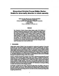
applied on CBM have not been developed well, are still the unsatisfied effectiveness and efficiency of H(S)MMs learning, mainly due to the lack of a method for optimizing the initial parameters of H(S)MMs to match observed signal patterns. Despite the drawbacks of poor initialization, classical iterative approaches such as the conventional Baum-Welch (BW) algorithm [11, 12] are still widely used to estimate H(S)MM parameters, for lack of alternatives. In order to decide an optimal state number, a lot of attempts have been made, such as using specific criteria (e.g. the Akaike information criterion (AIC) [13], the Bayesian Information Criterion (BIC) [14] etc.) and structure evolving method (e.g. The state splitting/ merging approach [15], the genetic approach [16]). However, the forementioned approaches usually bring the local optima risk and highly-computational load. In this study, we follow the idea of state-of-art heuristics learning, however different from the conventional BaumWelch algorithm starting with a randomly initialized H(S)MM model, we propose a Segmentation and Clustering (SnC) based identification approach to decide the number of states and the initial model parameters approximately. The approximate estimation is served as an effective starting point of the Baum-Welch algorithm which afterwards iteratively updates the initial parameters. We validated the proposed method on both synthetic and real industrial data. As it turns out, both the number of iterations needed and the chance of falling into a local optimum are reduced, representing the improved efficiency and effectiveness, respectively. 2. METHODOLOGY OF MODEL IDENTIFICATION As states reflect the behavior of a system, the persistence of states implies that the system exhibits the same behavior over a certain period which could be translated into the language of H(S)MMs that the recurrent state probability is high (above a certain threshold). Such time period in which the state of the system resides without change is called a regime. The proposed SnC algorithm identifies the regimes of a state using segmentation and clustering techniques. This paper focuses on industrial machinery systems which tend to stay in a stable and persistent state for a certain period before jumping to another state if no fault or failure occurs. The proposed SnC approach contains four steps, as de-

X SnC process Step 1: Identification of persistent states Signal

Step 2: Combination of states Step 3: Estimation of state numbers

Baum-Welch Learning

Step 4: Calculation of initial parameters

Fig. 1. Scheme of the SnC approach picted in Fig. 1. At first, signals are split into different regimes based on different signal behaviors. Secondly, ‘similar’ regimes of the signal are grouped together by clustering techniques according to their similarities. The achieved labeled regimes are assumed to be the hidden states. Thirdly, a clustering validation index is employed to determine the number of states. Finally, H(S)MM parameters are estimated by calculating statistical occurrences of the observed signal and the estimated hidden states, then used as initial input of the conventional Baum-Welch algorithm.

subsequence are used as initial starting centroids for k means clustering. Notably, 2) and 3) are the preliminary steps designed to avoid the problem of randomness in initializations of k-means clustering. 2.3. Step 3: Estimation of state numbers by cluster validity In order to select the optimal number of clusters, a robust index, called Davies-Bouldin index (DBI) [20], is applied in this paper. Suppose dataset X is partitioned into K disjoint nonempty clusters Ci and let {C1 , C2 , . . . , CK } denote the obtained partitions, such that Ci ∩ Cj = Ø (empty set), SK i 6= j, Ci 6= Ø and X = i=1 Ci . The Davies-Bouldin index [20] is defined as: K diam(Ci ) + diam(Cj ) 1 X max{ } DBI = K i=1 i6=j dist(Ci , Cj )

where diam(Ci ) = 2.1. Step 1: Identification of persistent states by segmentation Data sequences emitted by persistent states can be segmented into sub-sequences with constant behavior (observations follow a stationary distribution). The transition moment from one state to another can be identified by detecting a changepoint in signal behavior. In this paper, we propose a sliding window-based Bayesian segmentation for splitting discrete signals which employs the test of [17]. The test calculates the Bayesian probability that two sequences have been generated by the same or by a different multinomial model. The first sequence always starts from the last change point and ends at the current time point; the second sequence is a fixedlength sliding-window starting from the next time point. If the test indicates that the two sequences are generated from a different model with a confidence level, the current time point is marked as a change point. The procedure repeats until the end of the signal. Similar to the Bayesian segmentation, we employ a sliding window-based filter segmentation method for continuous signals, instead of using the Bayesian probability, the mean value difference of the two neighboring sequences is used as a change-points detector. 2.2. Step 2: Combination of states by clustering Regimes corresponding to the same state will recur over time. Assuming there is a finite number of states, segments with the same state are detected and clustered together. In this study, the classical k-means clustering approach [18, 19] is used to combine and label each segment, described as below: 1) feature points are computed by averaging the data in each segment; 2) the obtained feature points are divided into k subsequences with equal length; 3) the median values of each

min

xm ∈Ci ,xn ∈Cj ,i6=j

(1)

max {d(xm , xn )} and dist(Ci , Cj ) =

xm ,xn ∈Ci

{d(xm , xn )} denote the intra-cluster diam-

eter and the inter-cluster distance, respectively. Apparently, the partition with the minimum Davies-Bouldin index is considered as the optimal choice. 2.4. Step 4: Estimation of initial parameters The underlying assumption of our method is that segmentation of the observed signal allows us to identify quite accurately the regimes of the reference model. If the regimes belonging to the same state are grouped correctly, these regimes offer us good insight into the behavior of the states, i.e. the observation and transition probabilities as well as the duration distribution. The probabilities are estimated based on the observed frequencies. Parameters of an HMM (i.e., probability matrices) can be calculated by simple counting the occurrence of the observed signal and the hidden states (i.e., labels retrieved from clustering), which are computed as below [1, 11, 12]: π ¯i = frequency in state si at time t = 1 a ¯ij =

# of trans. from si to sj # of trans. from si

¯bj (k) = # of times in sj observing vk # of times in sj

(2) (3) (4)

where E is the expectation function and trans. is the abbreviation for transition. Note that Baum-Welch uses the same equations in (re)-estimating model parameters. Similarly, the parameters of an HSMM can be computed as below: π ¯i,d = frequency in state si at time t = 1, with dur. d (5)

# of trans. from si with dur. d0 to sj with dur. d # of trans. from si with dur. d0 (6) # of times o emitted in s t+1:t+d j ¯bj,d (ot+1:t+d ) = (7) # of times in sj

a ¯(i,d0 )(j,d) =

where dur. is the abbreviation for duration. The distribution of the duration d for each state can be modeled with both parametric and non-parametric approaches. Non-parametric modeling uses the kernel density estimation (KDE) based on a normal kernel function [21, 22]:

RU Llower =

N X

[µ(D(si )) − c × σ(D(si )))]

(11)

i=st

where st denotes the current state, ∀i ∈ state in the active path, c is the confidence coefficient, the CI is P (RU Llower ≤ RU L ≤ RU Lupper ). The accuracy of the RUL prediction is indicated by the root mean squared error (RMSE) criterion. This RMSE measure is useful to assess the prediction accuracy because of its sensibility to large errors.

γ

d − di 1 X KN ( ) f¯h (d) = γh i=1 h

(8)

where (d1 , d2 , . . . , dγ ) is a duration sample drawn from a distribution with density f , KN represents a normal kernel and h is bandwidth for the smoothing purpose, which is set as the optimal for normal densities. Parametric approach allows a predefined type of distributions such as Gaussian, Weibull, etc. and the corresponding distribution parameters. 3. VALIDATION We evaluate the proposed method in three aspects: learning accuracy, learning speed and prediction accuracy. The learning accuracy is indicated by the test-set likelihoods (LL) measure and the Local Optima Count (LOC) measure. The LL of the data given the model measures how well the model fits the data, i.e. log P (data|model). The LOC computes the number of models which are stuck in local optima. If the percentage of the LL difference with the reference HMM model is small (e.g. below a threshold of 5%), the model is considered as correctly learned, otherwise it is assumed to be a local optimum. The learning speed is represented by the learning time in seconds and the Iterations to Converge Count (ICC). The ICC is computes the number of iterations to converge. A shorter learning time and smaller ICC indicate a better running-time efficiency. The prediction accuracy is evaluated by the Remaining Useful Life (RUL) prediction. The RUL represents the expected useful lifetime left on an asset before a breakdown occurs, which is calculated using state duration parameters. A confidence interval (CI) is given using the standard deviation of the state duration. Three values of RUL according to CI is defined as [23]: RU Lmean =

N X

[µ(D(si ))]

(9)

i=st

RU Lupper =

N X i=st

[µ(D(si )) + c × σ(D(si )))]

(10)

3.1. Synthetic dataset We created 25 (5 × 5) random HMMs with a combination of 5 states and 5 observations both with range (2, 6). Each HMM is configured as persistent-state HMM and is used as a reference model to generate a synthetic dataset with 50 observation sequences of 500 time steps. The first 40 observation sequences are selected as training set and the remaining 10 are used as test set. In order to compare the identifiability performance, the conventional Baum-Welch algorithm and the proposed SnC method are used to learn each reference model. The number of states are selected from a state pool (2, 2 ∗ Q) for both approaches, where Q is the real state number. The Baum-Welch algorithm applies an AIC criterion for the number of state selection, while the SnC uses the DBI criterion. In the segmentation step of the SnC, the window size and the confidence level are set to 10 and 0.9, respectively. The threshold of the log-likelihood difference is set to 5% in this paper.

Table 1. Learning performance results obtained from the conventional Baum-Welch algorithm and the proposed SnC approach on synthetic data BW+AIC SnC Criteria 64 Topology Correct # states (%) 44 0.80 LL diff. (%) 2.06 Accuracy 0 LOC (%) 12 27.58 Learning time (s) 439.45 Speed 6.56 ICC (#) 10.50 As shown in Table 1, experimental results demonstrated that the SnC method outperforms the conventional BaumWelch algorithm. The SnC is more effective in learning, obtaining less LL difference and fewer number of local optima. Besides, it is more efficient, achieving a faster learning speed using less learning time and lower ICC. To visually see the improved performance of the proposed SnC method, a comparison of the encoding performance of the Viterbi path is shown in Figure. 2. Apparently, carefully initialized HMMs are closer to the reference models and fit the data better.

(a) Observed accelerometer signals Fig. 2. Example of the Viterbi paths encoded by the BW and the SnC methods on the last 150 samples of a test set

Run 1 Run 2 (b) RUL estimation using the Baum-Welch

Run 1 Run 2 (c) RUL estimation using the SnC 3.2. Real dataset The real data used in this experiment is collected from a Vertical Form Fill and Seal (VFFS) packing machine which produces bags of different food in food industry. As shown in Figure. 3, the VFFS machine supplies a plastic film roll which forms bags for packaging from a conical tube. A vertical heatsealing jaws bond the film and close the bag by mealing the seam together. After the bag is sealed, the film is cut by a knife to form a produced bag [24]. One of the major chalFig. 3. Seal quality monitoring in a packing machine [24]

lenge in this field is that the sealing quality degrades during the cutting process because of dirt accumulation and product leakage on the sealing jaws. Therefore, accelerometers are mounted on the jaws to detect the dirt accumulation. Maintenance activities are conducted by stopping the machine and cleaning the jaws [24]. In this study, we compared the proposed SnC method and the conventional Baum-Welch algorithm on the RUL prediction with HSMMs using the RMSE criterion. For the selection of number of hidden states, a state pool of (2, 6) are predefined. There are 11 runs with maintenance activities at the e’nd of each run, where from runs from 3 to 11 are used as training sets and runs 1 and run 2 are used as test sets. The results of the test-set RUL predictions with both approaches are shown in Fig. 4 and the RMSE results are shown in Table 2.

Run 1

Run 2

Fig. 4. Remaining Useful Life predictions

Table 2. Comparisons of the RUL prediction performance Method BW+AIC SnC Number of states 6 3 RMSE 284.3 111.1 Learning Time 2.2925 ∗ 103 5.7492 ∗ 102

The results obtained with the SnC approach are better performing with smaller RMSE estimation errors and less learning time compared to the conventional Baum-Welch algorithm. Moreover, the SnC selects a simpler model according to the number of states selected. The enhanced performance are gained via the good initialization estimated by the proposed SnC approach, which are obviously shown at the beginning of each run.

4. CONCLUSIONS When applying H(S)MM models to industrial applications, the random initialization for learning results in low efficiency and accuracy. This paper develops a segmentation and clustering based method, which properly initializes the number of hidden states and the model parameters for H(S)MMs. Our proposed method is validated by experiments with simulated and real data respectively, both obtaining satisfying results.

5. REFERENCES [1] Lawrence R. Rabiner, “A tutorial on hidden markov models and selected applications in speech recognition,” in Proceedings of the IEEE, 1989, pp. 257–286. [2] Shun zheng Yu, “Hidden semi-markov models,” Artificial Intelligence, 2010. [3] J. D. Ferguson, “Variable duration models for speech,” 1980. [4] A Verma, N Rajput, and LV Subramaniam, “Using viseme based acoustic models for speech driven lip synthesis,” in Acoustics, Speech, and Signal Processing, 2003. Proceedings.(ICASSP’03). 2003 IEEE International Conference on. IEEE, 2003, vol. 5, pp. V–720. [5] Beth Logan and Pedro Moreno, “Factorial hmms for acoustic modeling,” in International Conference on Acoustics, Speech, and Signal Processing, 1998, vol. 2. [6] Andreas Fischer, Kaspar Riesen, and Horst Bunke, “Graph similarity features for hmm-based handwriting recognition in historical documents,” in 2010 12th International Conference on Frontiers in Handwriting Recognition. Nov. 2010, vol. 0, pp. 253–258, IEEE. [7] Richard J. Boys, Daniel A. Henderson, and Darren J. Wilkinson, “Detecting Homogeneous Segments in DNA Sequences by Using Hidden Markov Models,” Journal of the Royal Statistical Society. Series C (Applied Statistics), vol. 49, no. 2, pp. 269–285, 2000.

[13] H. Akaike, “Information theory and an extension of the maximum likelihood principle,” in Second International Symposium on Information Theory, B. N. Petrov and F. Csaki, Eds. 1973, pp. 267–281, Akad´emiai Kiado. [14] Gideon Schwarz, “Estimating the dimension of a model,” The Annals of Statistics, vol. 6, no. 2, pp. 461– 464, 1978. [15] M. Ostendorf and H. Singer, “HMM topology design using maximum likelihood successive state splitting,” Computer Speech and Language, vol. 11, pp. 17–41, 1997. [16] Jonathan Goh, Lilian Tang, and L. Al turk, “Evolving the structure of Hidden Markov models for micro aneurysms detection,” in UK Workshop on Computational Intelligence, 2010. [17] Mathias Johansson and Tomas Olofsson, “Bayesian Model Selection for Markov, Hidden Markov, and Multinomial Models,” IEEE Signal Processing Letters, vol. 14, pp. 129–132, 2007. [18] J. MacQueen, “Some methods for classification and analysis of multivariate observations,” in Proc. Fifth Berkeley Symp. on Math. Statist. and Prob. 1967, vol. 1, pp. 281–297, Univ. of Calif. Press. [19] E. W. Forgy, “Cluster analysis of multivariate data: efficiency versus interpretability of classifications,” Biometrics, vol. 21, pp. 768–769, 1965.

[8] Jia Li, Amir Najmi, and Robert M. Gray, “Image classification by a two dimensional hidden markov model,” IEEE Transactions on Signal Processing, vol. 48, 2000.

[20] David L. Davies and Donald W. Bouldin, “A Cluster Separation Measure,” IEEE Transactions on Pattern Analysis and Machine Intelligence, vol. PAMI-1, no. 2, pp. 224–227, 1979.

[9] Jian bo Yu, “Health condition monitoring of machines based on hidden markov model and contribution analysis,” IEEE Transactions on Instrumentation and Measurement, vol. 61, pp. 2200 – 2211, 2012.

[21] Murray Rosenblatt, “Remarks on Some Nonparametric Estimates of a Density Function,” The Annals of Mathematical Statistics, vol. 27, no. 3, pp. 832–837, Sept. 1956.

[10] A. Jardine, D. Lin, and D. Banjevic, “A review on machinery diagnostics and prognostics implementing condition-based maintenance,” Mechanical Systems and Signal Processing, vol. 20, no. 7, pp. 1483–1510, Oct. 2006.

[22] Emanuel Parzen, “On Estimation of a Probability Density Function and Mode,” The Annals of Mathematical Statistics, vol. 33, no. 3, pp. 1065–1076, 1962.

[11] Leonard E. Baum and Ted Petrie, “Statistical Inference for Probabilistic Functions of Finite State Markov Chains,” The Annals of Mathematical Statistics, vol. 37, pp. 1554–1563, 1966. [12] Leonard E. Baum, Ted Petrie, George Soules, and Norman Weiss, “A Maximization Technique Occurring in the Statistical Analysis of Probabilistic Functions of Markov Chains,” The Annals of Mathematical Statistics, vol. 41, pp. 164–171, 1970.

[23] K. Medjaher, D. A. Tobon-mejia, and N. Zerhouni, “Remaining useful life estimation of critical components with application to bearings,” IEEE TRANSACTIONS ON RELIABILITY, pp. 292–302, 2012. [24] Adriaan Van Horenbeek, Abdellatif Bey-Temsamani, Steve Vandenplas, Liliane Pintelon, and Bart De Ketelaere, “Prognostics for optimal maintenance: Maintenance cost versus product quality optimization for industrial cases,” in World Congress on Engineering Asset Management (WCEAM 2011), 2011.