Tomlin et al. worked on hybrid system approach[4] for collision avoidance. Moreover ... In order to apply the PN guidance law to collision avoidance problems, a ...
2nd International Conference on Autonomous Robots and Agents December 13-15, 2004 Palmerston North, New Zealand
Proportional Navigation-Based Optimal Collision Avoidance for UAVs Su-Cheol Han, and Hyochoong Bang Division of Aerospace Engineering, Korea Advanced Institute of Science abd Technology, Daejeon, Republic of Korea {schan,hcbang}@fdcl.kaist.ac.kr
Abstract optimal collision avoidance algorithm for unmanned aerial vehicles based on proportional navigation guidance law is investigated in this paper. Although proportional navigation guidance law is widely used in missile guidance problems, it can be used in collision avoidance problem by guiding the relative velocity vector to collision avoidance vector. The optimal navigation coefficient can be obtained if obstacle moves with constant velocity vector. The convergence of proposed algorithm is also studied. The convergence can be obtained by choosing the proper navigation coefficient.
Keywords: collision avoidance, proportional navigation, optimal control, UAV 1 Introduction
use of the idea of total field to construct an avoidance algorithm[5].
Aircraft collision is a serious concern as the number of aircraft in operation increases. Ground air traffic control load has been also increasing due to heavy workload. In particular, UAV(Unmanned Aerial Vehicle)s may be additional flight objects for consideration of collision avoidance in the future. Autonomous UAVs will require sophisticated avoidance systems with conventional aircraft flying together. So far, most air traffic control is performed by ground station command. Ground air traffic controllers played a key role for safe operations of the air traffic flow.
In this study, a collision avoidance law based upon conventional PN(Proportional Navigation) guidance law is proposed. The PN guidance law is one of the most popular strategies for the missile engagement scenario[6]. In order to apply the PN guidance law to collision avoidance problems, a collision avoidance vector is defined first. Then the vector defining heading angle of the aircraft is guided to the collision avoidance vector defined. Convergence analysis of the PNCAG(Proportional Navigation-based Collision Avoid Guidance) was made to provide a condition for converging navigation constant. Moreover, optimal control theory was investigated to design an optimal navigation constant. For optimal navigation constant is employed to facilitate mathematical derivation[7].
However, with rapid increase of air traffic, the ground station-based air traffic control may not be sufficient to cover every flying object. Thus self-contained on-board air traffic control or collision avoidance systems have been considered. For autonomy of collision avoidance system requires avoidance laws among multiple aircraft in operation. The UAV or aircraft should carry active sensors which can detect other aircraft nearby. Information of other aircraft such as position, velocity, and heading angle can be used to design the avoidance command. Many collision avoidance law were proposed also for applications to robotics area. Katib proposed potential field-based approach for avoidance law design[1]. A series of follow-on research have been done using the potential field approach. Fuzzy logic algorithm was proposed by Tang et al. for a robot soccer problem[2]. Rathbun et al. applied the genetic algorithm[3] and Tomlin et al. worked on hybrid system approach[4] for collision avoidance. Moreover, Sigurd and How made
This paper consist of few section; first the principal idea of PNCAG is introduced, and sufficient condition for the collision avoidance is defined to finish the collision avoidance mode. In the next, selection of converging navigation constant is discussed. Design of optimal navigation constant using movable polar coordinate system is presented in the next section. In the next, simulation results are presented verifying the proposed algorithm.
2 PN-Based Collision Avoid Guidance 2.1 PNCAG Algorithm The key objective of collision avoidance is to maintain a predefined safe distance between the aircraft and
76
2nd International Conference on Autonomous Robots and Agents December 13-15, 2004 Palmerston North, New Zealand
obstacle. Configuration for the collision avoidance problem is presented in figure 1. An aircraft is facing a target aircraft classified as an obstacle in the two-dimensional plane.
avoidance law in equation (1) is essentially equivalent to the generic PN guidance law. In addition, it follows
θ˙ = φ˙ + γ˙ ¶ µ vrel sinψrel R˙T (tanφ + tanγ ) + =− RT RT cosφ
h ( xT , yT )
(2)
ψT RP
vT
i
Thus, the PN guidance command can be generated by using the information; vrel , ψrel , RT , φ , γ and R˙T
RT
γ
φ δ −vT vrel
2.2 Sufficient Condition for the Collision Avoidance
θ ψ rel v
ψ X = ( x, y )
Figure 1: Geometric configuration for the collision avoidance between two aircraft The obstacle cone is defined as a region formed by three points A,B,X in figure 1. The navigation mode denotes normal mode for which the aircraft fly over the designated course without obstacles. In the collision avoidance mode, the aircraft should perform collision avoidance maneuver on its route. With the geometric configuration in figure 1, summary of the PNCAG algorithm is presented in table 1 in the form of a pseudo code. Table 1: summary of PNCAG algorithm.
In this part, the sufficient condition for the collision avoidance is discussed. The collision avoidance condition must be defined to convert from collision avoidance mode to navigation mode when collision avoidance is accomplished. The sufficient condition for the collision avoidance is defined as follows; Condition 1 : The range between aircraft and obstacle is greater than safety distance (RP ). RT ≥ R P Condition 2 : The direction of the relative velocity (ψrel ) is outside of the obstacle cone. Condition 3 : The obstacle is located behind of the direction of the relative velocity vector.
ψrel
π ≥ + tan−1 2
µ
yT − y xT − x
or
¶ µ yT − y π ψrel ≤ − + tan−1 Do while (Aircraft does not reach the goal) xT − x 2 Calculate The sufficient condition for collision avoidance which vrel = v − vT if (Relative velocity vector is out of the obstacle cone) satisfies all conditions is illustrated in figure 2. Navigation mode is initiated Else Collision avoidance mode initiated 3-9 o’clock line End End Collision For collision avoidance, the so-called collision avoid−→ ance vector, XA in figure 1 is established first. Then the relative velocity vector between the aircraft and obstacle is steered toward the collision avoidance vector. Based upon the geometry of figure 1, the PN guidance command can be expressed as follows; a = Nvrel θ˙
avoidance vector
v
RP
vrel
(1)
where a is input acceleration, vrel relative velocity, θ represents the direction of collision avoidance vector, and N is the proportional navigation constant. The
vT
Obstacle cone
Figure 2: Sufficient condition for the collision avoidance.
77
2nd International Conference on Autonomous Robots and Agents December 13-15, 2004 Palmerston North, New Zealand
3 Convergence Analysis of PNCAG The PNCAG introduced above can be used effectively for the collision avoidance maneuver. Its performance has been verified already in a number of previous studies. In this section, convergence of the PNCAG law is investigated to ensure that the desired collision avoidance is accomplished by the proposed guidance law. For convergence analysis, figure 3 is introduced defining variables.
0 < θ − ψrel < π π 0 < θ − ψrel < → R˙ < 0 2 π < θ − ψrel < π → R˙ > 0 2
(6)
Therefore θ˙ is always greater than 0 in the collision situation. Now for the convergence analysis, let us introduce following definition as the error term
ξ = θ − ψrel
(7)
or
ξ˙ = θ˙ − ψ˙ rel
For the error term converge to 0, the time derivative of the error term always has negative value since the error term always has positive value in the collision situation as shown figure 3. If the feedback control input for collision avoidance is added to equation (8),then
Rα
α
R + ∆R
(8)
θ + ∆θ
R
ξ˙ = θ˙ − ψ˙ rel = (1 − N) θ˙
i
ξ θ
ψ rel
(9)
h
Figure 3: Geometry and associated variables for convergence analysis. In figure 3, the relative path of the aircraft is formed like the part shown in dotted line. So following equations are satisfied.
Rα sin (θ − α ) = R
sin (θ − α + ∆θ ) =
Rα Rα ' R R + ∆R
¶ µ ∆R 1− R
(3)
If the time interval ∆t is very small, then the point B approaches to the point A. So
∆θ = −
∆R tan (θ − α ) R
α ≈ ψrel
(4)
So following equation is satisfied R˙ θ˙ = − tan (θ − ψrel ) R
If the aircraft is faced with collision situation, then
In equation (9), since θ˙ is positive, then the following condition should be satisfied for the convergence N>1
(10)
4 Design of Optimal PNCAG In the previous section, basic concept for PNCAG and associated convergence analysis were elaborated. According to the convergence analysis, the guidance command guarantees convergence with the navigation constant greater than 1. in this section, optimization of the guidance law is discussed. The PNCAG law is optimized such that a given cost function is minimized to produce a particular guidance parameter such as optimal navigation constant. For the analysis of the optimal PNCAG a new formulation is considered by using a polar coordinate systems defined with respect to the collision avoidance vector. This facilitates the overall analysis without relying upon the inertial frame of reference. figure 4 shows the new coordinate system for formulation of relative dynamics. From the figure 4, the velocity components about the (~er , e~θ ) directions are obtained from
(5)
vr = −vrel cos (θ − ψrel ) + vT cos (θ − ψT ) vθ = vrel sin (θ − ψrel ) − vT sin (θ − ψT )
78
(11) (12)
2nd International Conference on Autonomous Robots and Agents December 13-15, 2004 Palmerston North, New Zealand
Based upon the cost function, the Hamiltonian of the system is constructed as
vT
ψT
H = K + (1 − K)N 2 (θ ) + λψ N(θ ) +λvr (vθ − vrel N(θ )sin(θ − ψrel ))
(20)
−λvθ (−vr − vrel N(θ )cos(θ − ψrel )) Application of the optimal control theory produces the following optimality condition
ψ rel
vrel
θ r er
2(1 − K)N(θ ) + λψ − λvr sin(θ − ψrel ) −λvθ vrel cos(θ − ψrel ) = 0
r eθ Figure 4: Polar coordinate system for the analysis of optimal PNCAG. Differentiation of equation (11) (12) results in
v˙r = −ψ˙ rel vrel sin (θ − ψrel ) + θ˙ vθ v˙θ = −ψ˙ rel vrel cos (θ − ψrel ) − θ˙ vr
(13)
(15)
Equation(13),(14) and(15) can be rewritten in terms of new independent variables (θ ) such that
= −N(θ )vrel sin (θ − ψrel ) + vθ = −N(θ )cos (θ − ψrel ) − vr
(16) (17)
= N(θ )
(18)
Now for optimization, the following cost function is proposed
θ0
2
K + (1 − K) N (θ ) d θ ¤
(19)
together with the constraints in euation (16),(17) and(18). The initial and final conditions are assumed to be given by
vr (θ0 ) = vr,0 , ψrel (θ0 ) = ψrel,0 ,
(22)
λv0r λv0θ
(23)
= λ vθ = λ vr
(24)
vθ (θ0 ) = vθ ,0 ψrel (θ f ) = θ f
λψ (t f ) = 0,
λvr (t f ) = 0,
λvθ (t f ) = f ree
(25)
Also, according to the optimal control theory, since the final θ f is free, H(t f ) = 0 also should be satisfied. As a consequence K +(1−K)N 2 + λvθ (−vr − v)relNcos(θ − ψrel )) = 0(26) From equation (23) and (24), it can be shown that
λvr (θ ) = Asin(θ − θ f ),
λvθ (θ ) = Acos(θ − θ f ) (27)
where A is a constant to be determined later. Substitution of equation (27) into equation (21) yields
0 = d ψ /d θ . where it is defined as ψrel rel
J=
λψ0 = −λvr vrel Ncosθ¯ + λvθ vrel Nsinθ¯
where θ¯ = θ − ψrel and the final conditions of the costate variables are given as
ψ˙ rel = N θ˙
Z θf £
The costate equations are also given by
(14)
In addition,
v0r vθ0 0 ψrel
(21)
N(θ ) = −
¢ ¡ 1 λψ − Avrel cos(θ f − ψrel ) 2(1 − K)
(28)
By taking derivative of equation (28) with respect to θ and using equation (22), the following relationship can be derived. N 0 (θ ) = −
¢ ¡ 0 1 λψ − Avrel N(θ )sin(θ f − ψrel ) = 0(29) 2(1 − K)
In other words, N(θ ) = const,
ψrel (θ ) = N θ +C
(30)
Since λvθ (t f ) = A in equation (27), it can be substituted into equation (26) so that it can ne solved for A
79
2nd International Conference on Autonomous Robots and Agents December 13-15, 2004 Palmerston North, New Zealand
A=
K + (1 − K)N 2 vT cos(θ f − ψT ) + vrel (N − 1)
(31)
Table 3: Simulation condition - Obstacle.
In equation (21) N=
1 Avrel 2(1 − K)
Initial position(km) Target position(km) Initial speed heading angle
(32)
Solving equation (31) and (32) together, we arrive at N = 1−µ ±
r
K + (1 − µ )2 1−K
Case I (-10,10) (10,10) 100 π /2
Case II (-4.7,14.7) (4.7,5.3) 100 −π /4
Case III (0,15) (0,5) 100 −π /2
(33)
where µ = vT cos(θ f − ψT )/vrel , Thus an equation for the optimal navigation constant is derived. Furthermore, from equation (30), the final angle satisfies
θf =
N θ0 − ψrel N −1
(34)
Thus the optimal navigation constant can be found by searching N which satisfy equation (33) and (34) in conjunction with equation (10). Nonlinear governing equations were used in deriving the optimal solution.
5 Simulation Results Simulation study is conducted to demonstrate the performance of the proposed collision avoidance algorithm. The aircraft is assumed to be a particle in the 2-dimensional plane. The corresponding dynamic equations of motion are given by
x(t) ˙ = v(t)cosψ (t)
(35)
y(t) ˙ = v(t)sinψ (t)
(36)
Figure 5: Simulation results for the Case I.
and
v(t) ˙ = −a(t)sin(ψrel (t) − ψ (t)) ψ˙ (t) = −a(t)cos(ψrel (t) − ψ (t))
(37) (38)
where ψ˙rel (t) = a(t)/vrel . The simulation conditions are given in table 2 and table 3 for aircraft and obstacles, respectively. Three different initial conditions are considered for simulation-Case I, Case II, Case III. Table 2: Simulation condition - Aircraft.
Initial position(km) Target position(km) Initial speed heading angle
Case I (0,0) (0,20) 100 π /2
Case II (0,0) (0,20) 150 π /2
Case III (0,0) (0,20) 200 π /2
Figure 6: Simulation results for the Case II.
6 Conclusion Collision avoidance guidance law motivated by conventional proportional navigation guidance is applied successfully to the collision avoidance of aircraft. The new guidance law was tested through convergence analysis and simulation study. From
80
2nd International Conference on Autonomous Robots and Agents December 13-15, 2004 Palmerston North, New Zealand
[4] Pappas G. Tomlin C. and Sastry S. Conflict resolution for air traffic manegement:a study in multiagent hybrid systems. Trans. IEEE Automatic Control, pages 509–521, April 1998. [5] Sigurd K. and How J. Uav trajectory design using total field collision avoidance. In proc. AIAA Guidance, Navigation, and Control Conference, August 2003. [6] Harry E. Criel Stephan A. Murtaugh. Fundamentals of proportional navigation. IEEE spectrum, December 1966. [7] Yang C. D. and Yang C. C. Optimal pure proportional navigation for maneuvering targets. IEEE Transaction on Aerospace and Electronics Systems, 33(3), July 1997.
8 Appendix the simulation results, the new method effectively achieve collision avoidance against the target aircraft with different initial conditions. PNCAG algorithm need velocity and position of the obstacle, and it can be easily obtained by radar or communication equipments. If we know above information we can easily apply this method to collision avoidance guidance. Although real-time optimal collision avoidance problem for moving obstacle is hard to solve, we can solve the above problem by PNCAG.
In this appendix the kinematic relationship for the collision avoidance angle in equation (2) is derived.
RP RT
7 Acknowledgements
y
`
Figure 7: Simulation results for the Case III.
This research was performed for the Smart UAV Development Program, one of 21st Centry Frontier R&D Program funded by the Ministry of Science and Technology of Korea.
θ γ
φ
x
References [1] khatib O. and Burdick. Motion and force control for robot manipulators. In proc. IEEE Robotics and Automation, pages 1381–1386, April 1986. [2] and Li X. Tang P., Yang Y. Dynamic obstacle avoidance based on fuzzy inference and principle for soccer robots. In IEEE, 10th International Conference on Fuzzy Systems, volume 3, pages 1062–1064, December 2001. [3] Pongpunwattana A. Rathbun D., Kragelund S. and Capozzi B. An evolution based path planning algrithm for autonomous motion of a uav through uncertain environments. In proc. IEEE Digital Avionics Systems Conference, volume 2, pages 8D2–1–8D2–12, 2002.
Figure 8: Geometric relationship of the angles. In figure 8, it follows as
x y , cosφ = RT RT RP sinγ = RT y˙ = −vrel sinψrel θ˙ = φ˙ + γ˙
sinφ =
(39)
(40) (41) (42)
Differentiate equation (40) and (41) with respect to time t and substitute equation (41) and (42) then, ¶ µ vrel sinψrel R˙T (43) (tanφ + tanγ ) + θ˙ = − RT RT cosφ
81