proposal for an indicative method for assessing and ...

European Journal of Environmental Sciences 

27

PROPOSAL FOR AN INDICATIVE METHOD FOR ASSESSING AND APPORTIONING THE SOURCE OF AIR POLLUTION V Í T Ě Z SL AV J I Ř Í K * , HA NA T OM Á ŠKOVÁ , O N D Ř E J M AC HAC Z KA , LU C I E K I S S OVÁ , BA R BA R A B Ř E Ž NÁ , A N D R E A DA L E C KÁ , and V L A D I M Í R JA N OU T Department of Epidemiology and Public Health, Faculty of Medicine, University of Ostrava, Syllabova 19, 703 00 Ostrava-Zábřeh, Czech Republic * Corresponding author: [email protected]

ABSTRACT The main objective was to provide a feasible approach for approximately apportioning the sources of air pollution based on simple calculations using measured concentrations of ambient air pollutants and meteorological data. The methods are based on dividing a monitored area into sectors using a common compass rose and obtaining hourly average concentrations of pollutants and relevant data on wind direction and speed over at least three seasons of a year. As a result, the relative contributions of all sources of air pollution in an area with a monitoring station are determined, together with the absolute contributions of single or groups of sources of pollution and the levels to which the emissions need to be reduced to meet the requirements of Directive 2008/50/ESt. The proposed methods are verified using data from measuring stations complying with that required by this Directive and are suitable for improving plans aimed at reducing air pollution as defined by the same document. This approach using data for a particular area revealed a total concentration of PM10 of 22.72 µg/m3, with the maximum permissible concentration of 12.33 µg/m3 this necessitates a reduction in concentration of the contributions from this selected group sources of 10.37 µg/m3. When these simple methods are used, further and more accurate apportionments of the source could be made using more complex mathematical modelling. However, this is only necessary in areas with many sources of pollution. Although these methods cannot compete with disperse and other types of modelling they may be useful in providing a basic overview of the situation in a particular area. Keywords: air pollution, PM10 concentration, source apportionment, Directive 2008/50/ES, pollutant monitoring, air quality improvement plans

Introduction Air pollution is an important environmental risk factor with an unquestionable adverse effect on human health (Amodio et al. 2009; Ruiz et al. 2011). The fact that the levels of risk to health from air pollutants are not negligible is mainly due to the political and economic status of a country with a sharp contrast between social pressure toward an acceptable air quality and the financial and economic pressures for sustaining production and consumption. The policy of a democratic, law-abiding state influenced by these two opposing forces usually seeks (from a historical perspective, at least temporarily) an equilibrium as expressed in its legislation (DIRECTIVE 2008/50/ EC 2008). Such an equilibrium, however, may be easily disturbed by inadequate inspection or adherence to the adopted legal norms. Yet an apparent problem in many countries (Mijić et al. 2009; Masiol et al. 2010; Unal et al. 2011), including the Czech Republic, is non-adherence to legal limits concerning ambient air pollutants. Health risks of ambient air pollutants acceptable for society are, among others, legislatively regulated by limit values for pollutants in the atmospheric boundary layer, particularly in residential areas or agglomerations (US EPA 2000). Legislation contains numerous requirements concerning acquisition and assessment of data on air

pollution. Thus, it might be said that from a legislative point of view, the issue has been resolved. Unfortunately, the opposite is true since the regulations do not answer the fundamental questions of what is the contribution of individual sources of pollution to the overall pollution in a particular area, for which sources corrective measures are needed to improve air quality and the extent to which the regulations are not adhered to in that area. Such solutions should be primarily fair, reliable and simple so that they could be implemented using data that are collected as required by the above legislation and thus are immediately available. Currently, the contribution to air pollution of individual sources is usually determined from data on sources of emission (Juda-Rezler et al. 2006; Srivastava et al. 2008; Viana et al. 2008; Thimmaiah et al. 2009; Mooibroek et al. 2011) using dispersion (diffusion) models (Perez-Roa et al. 2006). Given the fact that emissions are spread in the air by diffusion and flow of air and the relations describing these phenomena are relatively complicated (Cimorelli et al. 2004), dispersion models used to calculate air pollutant concentrations utilize many simplifications, leading to results different from the measured data. Although mathematical models are indispensable for predicting air pollution and additional calculations related to the measured data, this approach has other practical drawbacks. One example is the frequent unreliability of

Jiřík, V., Tomášková, H., Machaczka, O., Kissová, L., Břežná, B., Dalecká, A., Janout, V.: Proposal for an indicative method for assessing and apportioning the source of air pollution European Journal of Environmental Sciences, Vol. 7, No. 1, pp. 27–34 https://doi.org/10.14712/23361964.2017.3 © 2017 The Authors. This is an open-access article distributed under the terms of the Creative Commons Attribution License (http://creativecommons.org/licenses/by/4.0) which permits unrestricted use, distribution, and reproduction in any medium, provided the original author and source are credited.

28  Vítězslav Jiřík, Hana Tomášková, Ondřej Machaczka, Lucie Kissová, Barbara Břežná, Andrea Dalecká, Vladimír Janout officially reported data on emissions, another the irrelevant results of dispersion studies due to unavailable data on some sources of pollution in the monitored area. This article proposes methods that preferably use accurate data that are an increasingly reliable source of information on air pollution as compared with dispersion models and are thus, in accordance with valid legislation, a critical starting point for assessing higher emission loads, that is, those close to or beyond the limit values. The objective of the methods is to use as simple processing of the measured data as possible (Xiao et al. 2012) and additional dispersion models to estimate the contribution of individual sources of pollution in a particular area so that these data may be used as a starting point for adopting regional programs for reducing air polluting emissions, which determine mandatory corrective measures aimed at improving air quality and reducing risks to health.

Materials and Methods Measurements The input data set comprises hourly average concentrations (Ch) of ambient air pollutants. The approach is used for pollutants transported to a monitoring station in a particular area by diffusion and flow of air from all surrounding sources. Data on pollutant concentrations obtained from fixed monitoring stations are in accordance with Directive 2008/50/EC of the European Parliament

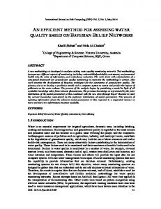
Fig. 2 An example of four monitoring stations and related wind roses.

European Journal of Environmental Sciences, Vol. 7, No. 1

N NW

NNW

NNE

NE

WNW

ENE

WSW

ESE

W

E

SW

SSW

SSE

SE

S

Fig. 1 Wind rose divided into 16 sectors.

and the Council (hereinafter the Directive) (Directive 2008/50/EC Chapter 5 2008) are, for the purposes of public health protection, considered valid and representative for the entire location. Hourly data on pollutant concentrations (Ch) and wind direction and speed must be acquired over a longer time period (Hrust et al. 2009) to eliminate seasonal and yearly fluctuations and ensure that the average concentrations over the entire period are really representative for the area. The longer time period refers to the time for which the Average Exposure Indicator is calculated in accordance with the Directive, for example, 3 years. A monitored area may be divided into sectors (k; directions as defined angles with vertices at a sampling point) according to the cardinal, intercardinal and secondary intercardinal points (Fig. 1).

𝑅𝑅! = under (3) !" ! calm ! frequencies Rk a Rs may be expressed !! wind conditions. !!! 𝑅𝑅!Relative = !!"!! (3) ! !!! !!!!! ! Rk a Rs may be expressed = !" frequencies(3) 𝑅𝑅!Relative !! !!! !! !!! (3) 𝑅𝑅assessing Proposal for an indicative method for and ! apportioning source of air pollution  29 ! = !" !!! !!! !! the(4) 𝑅𝑅! = 𝑅𝑅!!! (3) !" !!! ! !! ! = !" ! !! ! roses. Fig. 2 An example of four monitoring stations and related wind !!! ! !!!! ! 𝑅𝑅 = (4) ! !" ! Such division into sectors may be used for all moni𝑅𝑅! = !!!!"!!!! !!! (3) (3) 𝑅𝑅! = (4) tored areas, with sectors having their vertices at the sam- !" !!! !! !!! !! !!! !! !!! 𝑅𝑅! = !" (4) pling points (Fig. 2). !" ! !𝑅𝑅 with 1 (4) (5)wind air pollutant, hourly The data on hourly average concentrations (Ch) of an !  !𝑅𝑅! =average ! !!!+ (4) !!! 𝑅𝑅!!! ! = !" !" The data on hourly average concentrations (Ch) of an 𝑅𝑅!!!! !! +  !𝑅𝑅! = 1 (5) with !!! !!! ! air pollutant, hourly average and speed direction andwind speeddirection values may be used to calculate average concentrations 𝑅𝑅! = !"!" 𝑅𝑅 +   𝑅𝑅(C=k)(4) 1of the (5) with ! with ! !!! !!! ! !!! ! values may be used to calculate average concentrations !" Relative contributions P and P of the pollutant may 𝑅𝑅 +   𝑅𝑅 = 1 (5) with (5) pollutant for individual sectors over the entire time period as follows: k s ! !!! ! !" (Ck) of the pollutant for individual sectors over the entire with contributions 1 P(5) Relative k and s of the pollutant !!! 𝑅𝑅! +   𝑅𝑅!P= time period as follows: concentrations!"Ck and Cs of the pollutant and relevant may Relative contributions Relative Ppollutant and P(5) of the pollutant ks of spollutant with Pcontributions 𝑅𝑅!PCskof +  the 𝑅𝑅!C = 1 the k and and and rele concentrations !!! !! be estimated from average concentrations C and C of Relative contributions P and P of the pollutant may ! k s k s −3 !!! !! Cand ofkNand the pollutant and rele concentrations Ck and sP [μg mm−3] (1) 𝐶𝐶! = [µg ] (1) P of the pollutan Relative contributions the pollutant and relevant frequencies N , respecs k s !! ! ! Cs of the pollutant and relevant concentrations 𝑃𝑃! = !" ! !C!k !and (6) tively: ! ! ! ! !! ! Relative contributions P and Pspollutant of the pollutan k and re !!! 𝑃𝑃!concentrations = !!"! ! ! Ck and (6)Cs of the Where: !!! !! !!

!!! !!

! ! – k is the sector (each sector is an angle of 22.5°; see Ck and 𝑃𝑃!concentrations = !" ! !! ! !! (6)Cs of the pollutant and re (6) Where: ! ! ! !! ! ! !!! ! ! Fig. 1); 𝑃𝑃! = !" !! !! !! !!(6) !! !! !!! !! (7) !!!= 𝑃𝑃! Fig. = 𝑃𝑃1); – h is the hourly– value, or sector average(each valuesector per hour; (6) !" k is the is an angle of 22.5°; see ! ! ! !"!! ! !! !! ! ! !!! ! ! !!!!!!!! ! !!! (7) = (7) 𝑃𝑃 −3 ! !" ! ! !! !!! – Ckh [µg m ] is the hourly average concentration of the ! ! !! 𝑃𝑃! = !!!!"!!! !!! (6) – h air is the hourly or wind average value per hour;Concentrations !! !!C!!and !! frequencies N and N m pollutant in the at an hourlyvalue, average direc𝑃𝑃! = C!k and !" !!! s! ! (7) k s ! !! ! ! ! ! ! ! with !!! ! ! −3 tion uk > 0.5 m s−1 from sector k; 𝑃𝑃 = (7) !" –C [µg m ] is the hourly average concentration of the pollutant in the air at an hourly ! !" ! ! kh !! != +in!   !𝑃𝑃 1 (8) (8) area: with 𝑃𝑃!!! concentration C the !!!" ! monitored m!! =!!𝑃𝑃!!" (7) – Nk is the number (frequency) of hourly average wind !!!! !!! !!+!! with   𝑃𝑃 (8) −1 ! != ! 1 !!!𝑃𝑃 ! !!! 0.5 m s from sector k;Concentrations Ck!and average windconcentrations direction uk > C ! !! Cs and frequencies Nk and Ns m directions (and measured kh) over = (7) 𝑃𝑃 !"!" ! Cs 𝑃𝑃 and frequencies and Ns Concentrations Ck and!!! +   𝑃𝑃!! != with !!! !! !! ! 1 Nk(8) the entire time period from sector k; and !!! – Nk is the number (frequency) of hourlymay average wind directions (and measured !" theC !" in the monitored area: concentration be used to calculate average concentration Cm in m −3 ! ! !! ! 𝑃𝑃 +   𝑃𝑃 = 1 (8) with !!! – Ck [µg m ] is the average concentration of the pol!!! !!!!" ! !! 𝐶𝐶! = [µg m−3](8) (9) !" 𝑃𝑃 +   𝑃𝑃 = 1 with the monitored area: ! ! ! !! !!! lutant in the concentrations air over the entire period with an !!! Ckhtime ) over the entire time period from sector k; and! ! !" hourly average mean direction uk > 0.5 m s−1 from (8) with −3 !!! 𝑃𝑃! +   𝑃𝑃! = 1 !" the air – C [µg m ] is the average concentration of the pollutant in over the entire time k ! ! −3 !!! ! ! !!! !! −3 sector k. [μg m [µg ] (9) 𝐶𝐶! = m ] (9) !" !!! !!! !! Authors’ note:period The average or hourly median average value of amean set ofdirection uk >Similarly, with an 0.5 m s−1 concentration from sector k.contributions Dk and Ds may b data on concentrations of a pollutant should be calculated and Ps, respectively, kcontributions Similarly, Dofk and Dsand maythe average c The average or median of a contributions setconcentration of data on Pconcentrations a pollutant with regard to theAuthors’ statisticalnote: distribution of the data. When value be calculated, using either relative contributions Pk and Similarly, concentration contributions D k and Ds mayC determining average concentrations in with compliance Rdistribution and the determining average concentration k and Rs, respectively, should be calculated regardwith to the statistical of the data. When P , respectively, and the average concentration C or rels m legislation valid in EU countries, this approach is not used contributions Pk countries, and Ps, respectively, andisthe average ativelegislation frequencies Rk and and average average concentrations compliance valid in REU this the approach s, respectively, and the law requires that median values areincalculated as with : R , respectively, and−3the average concentration arithmetic means. Such an approach, however, is not sta- concentration Rk k=C and s = Rk Ck Pk k C [µg m means. ] (10) an m not used and the law requires that median values D are calculated as arithmetic Such tistically correct. −3] (10) D k = Pk Cm = Rk C Thus, the average C represent parThus,concentrations the average concentrations Ck represent partial concentrations ofk [μg the m pollutant at a approach, however, isk not statistically correct. −3 −3 tial concentrations of the pollutant at a sampling point [µgcircular (10) 4   D k= kC kC PP = =RasRC (11) −3m ] ] s= sC mm s k [µg m sampling point in aairmonitored carried by theDair flow from particular sector D s = Ps Cm = Rs Cs [μg m ] (11) in a monitored area carried by the flow from area a par−1 −1 ticular circular downwind sector downwind if the wind if the wind speed is ūspeed h > 0.5 m s . Under calm wind conditions, i.e. ūh ≤ 0.5 m s ,   with −1 −3 is ūh > 0.5 m s . Under calm wind conditions, i.e. Ds = P!" ] (11) s Cm = Rs C s =[µg 𝐷𝐷 𝐶𝐶!m (12) (12) point (Cwith theaverage average concentration at sampling the sampling as   follows: ! !!! 𝐷𝐷! + s) is calculated ūh ≤ 0.5 m s−1, the concentration at the point (Cs) is calculated as follows: This approach corresponds with that used in disper!" with +(yearly)   𝐷𝐷! = 𝐶𝐶 !! ! (12) sion models where long-term concentrations !!! 𝐷𝐷! This approach corresponds with that usedofin dispersion −3 !!! !!! −3 [µgmm ] (2) ] (2) 𝐶𝐶! = ! [μg a pollutant are the sum of contributions corresponding ! concentrations of a pollutant are the sum of contributio to concentrations for individual standardized meteoro−3 Where Csh [µg m ] is the hourly average concentra- logical situations This approach corresponds with that used multiplied by the average frequency of in dispersio individual standardized meteorological situations multi tion of the pollutant under calm −3 wind conditions, i.e. these situations (Bubník et al. 1998). As is the case with Where Csh [µg m ] is the hourly average concentration of the pollutant calm wind concentrations of et aRpollutant are sumcase of contributi uk ≤ 0.5 m s−1 (US EPA 2000), and Ns is the number (fre- D and D situations (Bubník al.under 1998). Asathe is the with Dk a , relative frequencies and Rs and selected k s k −1 quency) of concentrations C measured over the entire andand Ns amay isselected thebenumber of be used conditions, shi.e. uk ≤ 0.5 m s (US EPA 2000), limit value LV used to (frequency) determine perindividual standardized situations mul limit valuemeteorological LVmaximum may to determin period. The lower and upper limits of the confidence missible concentration contributions D and D , k,max s,max concentrations Csh95%) measured the entire period.situations The lower(Bubník and upper limits of the et al. As is the case with Dk interval (at a significance level of for theover average contributions Dk,max and D1998). respectively: s,max, respectively: concentrations Cconfidence referred(at to aassignificance Ck95L, Ck95H, level of 95%) for the average concentrations Ck and Cs k and Cs areinterval and a selected limit value LV may be used to determi Cs95L and Cs95H, respectively. These may be used to de- Dk,max = Rk LV [μg m−3] (13) Ck95H, Cs95L and Cs95H, respectively. TheseDk,max may be to, respectively: determine are referred to as Ck95L termine the significance of differences in, concentrations Ds,max Dcontributions m−3and ] used (13) k,max = Rk LV [µg between individual sectors or concentrations under calm Ds,max = Rs LV [μg m−3] (14) the significance of differences in concentrations between Ds,max = individual Rs LV [µg sectors m−3] or concentrations (14) wind conditions. −3D or D are greater If concentration contributions under calm wind Relative frequencies Rk and Rs conditions. may be expressed as s (13) Dk,max = Rk LV [µg m ]k than maximum permissible concentration contributions quotients: −3

Relative frequencies Rk a Rs may be expressed as quotients: [µg m ] (14) s,max = Rs LV contributions IfDconcentration D k or Ds are greater than European Journal of Environmental Sciences, Vol. 7, No. 1

𝑅𝑅! =

!! !" ! !!! !

!!!

(3)

contributions Dk,max and Ds,max, respectively, necessary If concentration contributions Dksimply or Ds are greater tha contributions in sectors k may be determined as

contributions Dk,max and Ds,max, respectively, necessar

with

!!!

!!!

𝐷𝐷!"#,!"# = 𝐷𝐷!,!"# (21)

permissible concentration contribution Ds among all the co

(20) Dskj,max = Ds / (Nkj · 16) 30  Vítězslav Jiřík, Hana Tomášková, Ondřej Machaczka, Lucie Kissová, Barbara Břežná, AndreaTherefore, Dalecká, Vladimírtotal Janoutmaximum permissible contributions of

Dk,max and Ds,max, respectively, necessary reductions in concentration contributions in sectors k may be simply determined as follows: ΔDk = Dk − Dk,max [μg m−3] (15)

= D / (N · 16)

D

(20)

skj,max !!" s kj follows: 𝐷𝐷!"#,!"# D = Ds=/ (N kj ∙ 16) (21) 𝐷𝐷!,!"# with !" !!! !!!skj,max



with

(20)

!!"

!" !!" with (21) (21) !,!"# !!! !!! Therefore, total maximum permissible of[µg sources = 𝐷𝐷 𝐷𝐷!"#,!"# += 𝐷𝐷 𝐷𝐷contributions m−3]in 𝐷𝐷!,!"#,!"! !,!"# !!! !"#,!"#

No reductions in emission contributions are needed if ΔDk ≤total 0 and ΔDs ≤ 0.permissible Concentration follows: Therefore, maximum contributions −3] (16) of sources in sectors k are calculated as follows: = D − D [μg m ΔD s sD may s,max be considered as minimum since contributions they do not involve contributions from Therefore, total maximum permissible contributions of so

0 and ΔDreductions No reductionsk in emission contributions are needed if Total ΔDk ≤necessary in concentration contributio s ≤ 0. Concentration !!" ≤ 0 and ΔD ≤ 0. Concentration No reductions in emission contributions are needed if ΔD k s sources under calm wind conditions although they affect the area. This is expressed follows: = 𝐷𝐷 𝐷𝐷!"#,!"#by [µg m−3] (22) [μg m−3 ] (22) No reductions in emission contributions are needed !!! contributions contributions Dk may be considered as minimum𝐷𝐷!,!"#,!"! since they do!,!"# not involve from calculated as:+ if ΔDk ≤ 0 and ΔD ≤ 0. Concentration contributions D s k contributions Dk may be D considered since contributions they do not involve contributions from allminimum concentration from all surrounding concentration contribution s, a sum ofas sourcesasunder calmsince windthey conditions although they affect the area. This isinexpressed by contribumay be considered minimum do not involve Total necessary reductions concentration !calculated sources under calm wind conditions althoughtions they affect thetoarea. Thisadequate is expressed byas:contributions !" information −3 all sou contributions from under calm wind conditions of𝐷𝐷 all sources in sectors k+in are sources in sources the area under calm conditions that is unable provide Total necessary reductions concentration −3 mof ] concentration contribution Dwind contributions from all 𝐷𝐷 surrounding ΔD − D [µg m ] [µg(23) !,!"#,!"! !,!"# !"#,!"# s, a sum of all concentration k,tot ==D𝐷𝐷 k,tot k,max,tot !!! although they affect the area. This is expressed by conconcentration contribution Ds, aindividual sum of allsectors concentration contributions from surrounding calculated as: about contributions sources k. This contribution may beall apportioned centration contribution ΔD , a of sum of calm all in concentration [μg information m−3] (23) sources in theDsarea under wind conditions that is unable toDprovide adequate k,tot = k,tot − Dk,max,tot contributions from all the surrounding sources in the area sources in area under calm wind conditions that is unable to provide adequate information among individual sectors or sources using approaches forThis calm wind periods in be dispersion contributions sources individual k. contribution may If anecessary selected sector k Ncontains Nkjansources, an adequate reductions inapportioned concentration contributions under calmabout wind conditions that of is unable to in provide ad- sectors sources, adequate If a Total selected sector k contains −3 kj =This Dk,totcontribution − Dk,max,tot may [µgbemapportioned ] (23) ΔDk,tot about contributions of sources in individual sectors k. models (Bubník et al. 1998). equate information about contributions sources in in- approaches dispersion model, i.e. calculation, may be usedconcentration to deteramong individual sectors orofsources using for calm periodsthe inrelevant dispersion be used towind determine contrib calculated as: dividual The sectors k. This contribution may be apportioned mine the relevant concentration contributions D (calc) kj among individual sectors or sources using approaches for calm wind periods in dispersion total concentration Ds over a calm wind period may be roughly apportioned models (Bubník et al.contribution 1998). In this case, on concentrations obtained among individual sectors or sources using approaches for valid thepoint. sampling In data this data on concen-aredispersion sources, an adequate m If aatselected sectorpoint. k contains Nkjcase, models (Bubník et al. 1998). among sectors k or individual sources according to the formula, assuming that−3but thefrom a calm wind periods inconcentration dispersion models (BubníkjD et al. trations arefollowing obtained not from measurements The total contribution wind period may be roughly apportioned dispersion model and may not therefore be valid (see th s over a calmΔD = Dk,tot − D [µg m ] contributions (23) k,max,tot be usedk,tot to determine the relevant concentration Dkj(c 1998). dispersion model and may may not therefore be valid (see the a calm wind period be roughly apportioned The total concentration contribution Dsaover emission flow of the pollutant resembles cylinder with radius X and height L: sectors kcontribution or individual j according tostated the following formula, assuming the be not Validity dispersion model may simply The totalamong concentration Ds sources reasons in case, theof Introduction). Validityresults ofthat dispersion over a calm point. In this data on concentrations are obtained fromver m or individual sources j according the following formula, assuming that the modelto results may be simply verified using the following wind periodamong may besectors roughlyk apportioned among sectors emission flow of the pollutant resembles a cylinder radius Xup and height L: Ncontributions summing concentration (calc): kj sources, anDadequate disp Ifwith afor selected kconcentration contains dispersion modelsector and may not therefore be valid (see the reasons s kj contributions summing up k or individual sources j!according to the following for- formula ∙!"∙! ! pollutant resembles !"of emission flow the a cylinder with radius X and height L: −3 [µgthe m pollutant ] (17) 𝐷𝐷!"# (𝑐𝑐𝑐𝑐𝑐𝑐𝑐𝑐) Dkj(calc): mula, assuming that ≅ the emission flow of Validity of dispersion model mayconcentration be simply verified using be used to determine theresults relevant contributi !!∙! ! ∙! !" resembles a cylinder with radius X and height L: ! ∙!"∙!

𝐷𝐷!"# (𝑐𝑐𝑐𝑐𝑐𝑐𝑐𝑐) ≅ !!" ∙!"∙! [µg m−3] ! !!∙! !" !" ∙!! 𝐷𝐷!"# (𝑐𝑐𝑐𝑐𝑐𝑐𝑐𝑐)! ≅ !!∙! ! ∙! [μg m−3[µg m−3] ] (17) !" !" !" with !!! !!! 𝐷𝐷!"# = 𝐷𝐷! (18) !



!" concentration contributions −3 summing Dkj(calc): point. up In 𝐷𝐷this(𝑐𝑐𝑐𝑐𝑐𝑐𝑐𝑐) case, data concentrations (17) ] (24) = 𝐷𝐷on [µg m−3] are obtained (24) not !,!"! [μg m !!! !" (17) dispersion model and may not therefore be valid (see the r

!

If !the relation is not fulfilled, data on concentrations !" −3 𝐷𝐷dispersion =model 𝐷𝐷!,!"! do model [µgcorrespond mresults ] (24) !" (𝑐𝑐𝑐𝑐𝑐𝑐𝑐𝑐) Validity of dispersion bethe simply verifie from!!! the not with If the relation is not fulfilled, datamay on concentrations fro !!" !" measured data and model calculation results have to be (18) with !!! !!! 𝐷𝐷 = 𝐷𝐷 (18) ! !!" !"# summing up concentration contributions D !" kj(calc): with the measured data and model calculati corrected.correspond Necessary reductions in concentration contri𝐷𝐷 = 𝐷𝐷 (18) !!! !!! !"# flow! of a source Qkj [t/year] and its distance from a sampling point Xkj In with addition to emission If the relation is not fulfilled, data on concentrations In addition to emission flow of a source Qkj [t/year] bution ΔDkj of a source in the monitored area may befrom the dispe Necessary reductions in case concentration contribution ΔD the calm wind [m], a concentration contribution is also onanalogically duration and its distance from atosampling point Xof determined to those in ofmodel ΔDk, as such a dependent s of kj [m], correspond the T measured data and results h !!" itswith In such addition emission flow a source Q and distance from a sampling point Xkjseen kj [t/year] −3 calculation 𝐷𝐷 (𝑐𝑐𝑐𝑐𝑐𝑐𝑐𝑐) =from 𝐷𝐷!,!"! [µg mpoint ] those (24) concentration contribution is also dependent on durafrom formula (15): may determined analogically to in case of ΔD !"be !!! [t/year] and its distance a sampling X In addition to emission flow of a source Q kj kj period and the average heightaverage of theheight atmospheric mixed layer Lduration [m] (US EPA 1999). Necessary reductions inTsconcentration contribution ΔDkj of a sourc [m], such a concentration isofalso dependent on of the calm The wind tion Ts of the calm wind period and the contribution −3] (25) [m], such a layer concentration is× also on T–only ofk,max,tot the calm wind the atmospheric mixed L [m] (UScontribution EPA 1999). The Dkjthis (calc) [μg m sD conversion factor CF is 114,155.25 [year µg ΔD / dependent h may ×mixed t].be Although is(US a rough estimate determined analogically to those in case of ΔDk, as seen fro kj =duration period and the average height of the atmospheric layer L [m] EPA 1999). The conversion factor CF is 114,155.25 [year × µg / h × t]. If the relation is not fulfilled, data on period and the average height of the atmospheric mixed(alayer L accurate [m] (US EPA 1999). Theconcentrations from it does not consider, instance, the[year height of /sources more estimate requires Althoughasthis is only a rough as it does not conAdditionally, a suitable model and the necconversion factorestimate CFfor is 114,155.25 × µg h × t]. Although this dispersion is only a rough estimate the dataas and model sider, forthe instance, height sources (afor more accurate essary reductions inwith concentration in the calculation conversion factorofCF is 114,155.25 [year ×conditions), µg / h ×correspond t].itAlthough this ismeasured only acontributions rough estimate use ofthe a dispersion model calm wind is(asufficient for theestimate purpose seen as it does not consider, for instance, the height of sources more accurate requires estimate requires the use of a dispersion model for calm particular area may be used to determine necessary reNecessary reductions inincreased concentration contribution ΔDkj o as it does not consider, for reliability instance,asthe height of sources (a more accurate estimate from data. the estimate may ifrequires wind conditions), forThe the purpose seen ductions of emissions for eachfor source, potentially leading the experimental useitofis asufficient dispersion model for calmof wind conditions), itbeisconsiderably sufficient the purpose as seen from experimental data. The reliability of the estimate to adherence to the adopted limit values. may be determined analogically to those in case of ΔDk, a the use sources of a dispersion model for wind conditions), it is sufficient for the(15) purpose nearly are considered andcalm the fulfillment of themay condition in formula mayifas be seen fromall experimental Theall reliability of the estimate be considerably increased may be considerably increased data. if nearly sources are from experimental The reliability of theEquipment estimate and may be considerably increased if verified. considered and the fulfillment ofdata. condition in formunearly all sources aretheconsidered and the fulfillment of theSoftware condition in formula (15) may be la (15) may be verified. To verify the methods, data from monitoring nearly all sources contributions are consideredofand the fulfillment (15) may stations be concentration sectorsofkthe arecondition calculatedinasformula follows: verified. Thus, Thus, concentration contributions of sources jsources in sec- j in were processed with the statistical software Stata (Stata verified.as follows: tors k are calculated Corp., Release 9, College Station, Texas, USA) and the Thus, concentration contributions of sources spreadsheet j in sectors kprogram are calculated as follows: Excel (Microsoft Corp., World!!" Thus, concentration contributions of sources j in sectors k are calculated as follows: −3 −3] (19) wide, USA). 𝐷𝐷!,!"! = 𝐷𝐷! + !!! 𝐷𝐷!"# [μg m [µg m ] (19) with

!!"

is the=number sources where N𝐷𝐷 𝐷𝐷! + of!!! 𝐷𝐷 j in sector [µg mk.−3] (19) kj !,!"! !!" !"# −3 Maximum permissible concentration contributions of Results = 𝐷𝐷 + 𝐷𝐷 [µg m ] 𝐷𝐷 !,!"! ! number !!! !"# where Nkj is the of sources j in sector k.(19) individual sources under calm wind conditions may be roughly estimated sectors kofbysources evenly japporwhere Ninkj sixteen is the number in sector k.The above methods were verified using experimental tioning maximum permissible concentration contribuwhere Nkj is the number of sources j in sectordata k. from measuring stations in some boroughs of the 7   tion Ds among all the considered sources j: city of Ostrava included in the national network consis-

European Journal of Environmental Sciences, Vol. 7, No. 1

  7   7      

Proposal for an indicative method for assessing and apportioning the source of air pollution 

31

Fig. 3 Average concentrations of PM10 in the air obtained from measuring station B in winter and summer.

Fig. 4 Average concentrations of NO2 in the air obtained from measuring station B in winter and summer.

tent with the Directive. The measuring station in one of the city boroughs (Radvanice and Bartovice) is referred to as B in Fig. 2. In this as well as other areas of the city, measuring stations recorded readings above limit values for pollutants, especially particulate matter. All hourly average concentrations and data on wind direction and speed were obtained over several years (all seasons over a period of six years). Data used to verify the above method are graphically summarized in Fig. 3 for PM10 and in Fig. 4 for NO2. The detailed results are listed only for PM10 in numerical form because of the possible scope of the article, as a demonstration of the above method.

Table 1 clearly shows that relative contributions of pollutants from sectors k = 10, 11 and 12 are ΣPk = 0.34 and relative contributions from all sectors under calm wind conditions are Ps = 0.30. This corresponds with concentration contributions ΣDk = 20.28 [μg/m3] and Ds = 17.85 [μg/m3]. If maximum permissible concentration contributions are Dk,max = 9.91 [μg/m3] for these three sources and Ds,max = 12.88 [μg/m3] for all sectors under calm wind conditions, the necessary reductions in concentration contributions are ΔD10,11,12 = 10.37 [μg/m3] and ΔDs = 4.97 [μg/m3], respectively. There are numerous important sources of pollution in Ostrava. To illustrate the application of the above meth-

Table 1 Parameters of the proposed method for PM10 obtained from the B measuring station. PM10 Limit value [µg m−3] = 40 Units

–

–

[µg m−3]

Sector k

Nk

Rk

Ck95L

Ck95H

Ck

Pk

Dk

Dk,max

ΔDk

1

1301

0.0311

45.31

48.85

47.08

0.0243

1.47

1.25

0.22

2

2255

0.0540

43.96

46.90

45.43

0.0407

2.45

2.16

0.29

3

2588

0.0619

44.74

47.56

46.15

0.0474

2.86

2.48

0.38

4

1566

0.0375

51.76

57.04

54.40

0.0338

2.04

1.50

0.54

5

965

0.0231

53.00

58.68

55.84

0.0214

1.29

0.92

0.37

6

1013

0.0242

39.79

43.53

41.66

0.0168

1.01

0.97

0.04

7

724

0.0173

37.60

41.58

39.59

0.0114

0.69

0.69

−0.01

8

582

0.0139

36.34

40.72

38.53

0.0089

0.54

0.56

−0.02

9

981

0.0235

37.23

41.05

39.14

0.0152

0.92

0.94

−0.02

10

2265

0.0542

50.15

53.09

51.62

0.0464

2.80

2.17

0.63

11

3437

0.0822

87.15

90.51

88.83

0.1212

7.31

3.29

4.02

12

4655

0.1114

89.77

92.91

91.34

0.1688

10.17

4.46

5.72

13

2445

0.0585

46.14

49.00

47.57

0.0462

2.78

2.34

0.44

14

1017

0.0243

45.15

49.82

47.49

0.0192

1.16

0.97

0.18

15

1247

0.0298

77.02

85.08

81.05

0.0401

2.42

1.19

1.22

16

1290

0.0309

78.90

85.52

82.21

0.0421

2.54

1.23

1.30

Forwind Windless Total

[µg m−3]

[µg m−3]

–

[µg m−3]

[µg m−3]

[µg m−3]

∑Nk

∑Rk

Cw95L

Cw95H

Cw

∑Pk

∑Dk

∑Dk,max

∑ΔDk

28331

0.6779

60.67

64.50

62.58

0.7039

42.43

27.12

15.31

Ns

Rs

Cs95L

Cs95H

Cs

Ps

Ds

Ds,max

ΔDs

13461

0.3221

54.67

56.17

55.42

0.2961

17.85

12.88

4.97

∑Nk+Ns

∑Rk+Rs

Cm95L

Cm95H

Cm

∑Pk+Ps

∑Dk+Ds

∑Dk,max+Ds,max

∑ΔDk+ΔDs

41792

1.0000

58.74

61.81

60.28

1.0000

60.28

40.00

20.28

European Journal of Environmental Sciences, Vol. 7, No. 1

32  Vítězslav Jiřík, Hana Tomášková, Ondřej Machaczka, Lucie Kissová, Barbara Břežná, Andrea Dalecká, Vladimír Janout

Fig. 5 Distribution of pollution sources around measuring station B.

od, several sources of pollution in Plant X were selected which are found in sectors k = 10, 11 and 12 (see Fig. 5). Concentration contribution Ds and the relevant necessary reduction ΔDs for all sources under calm wind conditions may be divided into concentration contributions for individual sources Dskj and necessary reductions in concentration contributions for individual sources under calm wind conditions ΔDskj using formulae (17) to (22). For sources shown in Fig. 5, characterized by variables Qkj = 1246.48 [t/year], Xkj = 2599 [m] for distances of sources from the sampling point from 1570 up to 3670 meters, Ts = 50 [h], L = 200 [m] (CHMI, 2008), are calculated: Dskj = 1.27 [μg/m3], Dskj,max = 2,42 [μg/m3] and ΔDskj = −1.14[μg/m3]. Thus, the total concentration contribution for all sources in sectors k = 10, 11 and 12 is Dk,tot = 20.28 + 1.27 = 21.55 [μg/m3], the maximum permissible concentration contribution is Dkmax,tot = 9.91 + 2.42 = 12.33 [μg/m3] and ΔDk,tot = 10.37 + (−1.14) = 21.55 − 12.33 = 9.22 [μg/m3]. This example is described in order to establish the validity of the above method.

Discussion The above methods propose several parameters simply describe the estimation of concentration contributions of individual sources or groups of sources to pollution of a particular area. Such pollution, if approximately equal to or greater than the limit values, must be, in accordance with the Directive (DIRECTIVE 2008/50; EC 2008) assessed using measured data and not dispersion (Bubník 1998; Cimorelli et al. 2004) or receptor (Hopke et al. 2010; Zeng et al. 2010) modelling. This rule is respected by the proposed methods and the parameters are calculated exclusively from measured data and modelling may only be used to obtain more accurate results. The basic parameter of the methods is relative contribution Pk of a selected pollutant brought to the monitored area from a particular direction (i.e. sector k; see formulae (1) to (6) in section Measurements, if the wind speed is >0.5 m/s (i.e. not under calm wind conditions; European Journal of Environmental Sciences, Vol. 7, No. 1

see below) (Donnelly et al. 2011; Henry et al. 2012). To determine this parameter, more detailed measured data should be used, such as hourly average concentrations and corresponding hourly average wind direction and speed values over a longer time period. Given the relatively large amount of such data (theoretically, 365 days × 24 hours = 8,760 hourly values), high statistical power of the results may be assumed; fluctuations in annual data (from all seasons) should be compensated for by using data obtained over three or more years (similar to the Average Exposure Indicator as defined by the Directive). In the present study, hourly values obtained over six years were used, with the number of values (sum of Nk) from a single measuring station exceeding 40,000 (see Table 1). Concentration contribution Dk of a pollutant is simply calculated from relative contribution Pk and average concentration in the area Cm, see formula (10). The above parameters are not valid under calm wind conditions, that is, if wind speed exceeds 0.5 m/s. Although this value was also experimentally determined in this study, the results are beyond the scope of this article. Since the value found in the present study is consistent with that published by the US EPA (AERMOD, 2004), calm wind conditions were defined as wind speed ≤ 0.5 m/s. Given the fact that under calm wind conditions, all neighbouring sources contribute to pollution at the sampling site, parameters for all sources in the area together were first calculated, that is, relative contribution Ps using formula (7), concentration contribution Ds using formula (11) and maximum permissible concentration contribution Dsmax using formula (14), and then apportioned among individual sources. For such apportionment, the following must be known: emission flow of sources of the pollutant Qkj, distance of sources from the sampling point Xkj, height of the atmospheric boundary layer L and average duration of calm wind periods Ts. Although this is only a rough approximation that may not provide accurate results for areas and sources that differ considerably in height, our experiences have shown that it is likely to be applicable in most cases. However, it must be remembered that the calculation is only used for calm wind conditions, which are rather sporadic in some areas. In the area monitored in the present study, calm wind conditions accounted for approximately 30% of the 6-year period (see Rs in Table 1), that is, they were relatively very common (the monitored area is known for frequent and long periods of smog and calm wind). Yet, based on our experiences with monitoring and dispersion modelling, the results obtained with the aforementioned methods are not far from the truth. The average height of the atmospheric mixed layer L may be calculated or measured (US EPA 1999). The proposed methods have been practically verified by calculations using accurate data. The article shows sample calculations related to several sources of pollution within a single large industrial Plant X on the outskirts of a city (a population of approximately 300,000) and a

Proposal for an indicative method for assessing and apportioning the source of air pollution 

measuring station located in a residential area considerably affected by them. The long-term average concentration of PM10 was 60.3 μg/m3, with the limit value being set at 40 μg/m3. Thus, to meet the limit value, the amount of particulate matter emissions from the sources in the plant would have to be reduced by ΔDk = 10.37 [μg/m3] under windy conditions and by ΔDskj = −1.14 [μg/m3] under calm conditions at the site of the measuring station, that is, by a total of ΔDk,tot = 9.22 [μg/m3]. To achieve the total necessary reduction in concentration contributions ΣΔDk + ΔDs = 20.28 [μg/m3], the other sources account for the remaining reduction by 11.06 [μg/m3]. Data on the necessary reduction of concentration contributions ΔDk,tot may be used by the source operator to model the amount of pollutants emitted by the source to meet the limit values for pollutants in ambient air, that is, not only the emission limits. Moreover, these data should include national and regional action plans that, in accordance with the Directive, should ensure that the population is exposed to acceptable air pollutant levels over a defined period of time. If the plans for reducing concentrations of air pollutants only contain technical measures to reduce emissions and the unsatisfactory condition is not corrected over time, the source operator remains unpunished and the population continues to be exposed to increased health risks.

Conclusion The presented approximate source apportionment is a simple mathematical application using measured data available from any measuring station compliant with Directive 2008/50/EC, that is, where limit values for ambient air pollutants are exceeded. Data on concentrations of ambient air pollutants, corresponding meteorological data and some available data on sources of air pollution and their groups are used to calculate concentration contributions of selected pollutants relevant to individual sources. Subsequently, necessary reduction of these concentrations is determined so that the total contribution of all sources does not exceed the limit values defined by the Directive. The methodology was tested using data relevant to a particular source of pollutants. Although the above methods are only a first approximation for obtaining information on source apportionment in a monitored area they may be a sufficient and fair starting point for developing air quality plans in accordance with the Directive. Unfortunately, the document does not contain even minimal guidance on how to make individual source operators reduce their emissions. If air quality plans developed in accordance with the Directive comprised requirements for reduction of concentration contributions, the presented approximate methods could be used to determine maximum permissible concentration contributions of every source more accurately so that the limit values are adhered to. The presented cal-

33

culations for a selected group of sources within a single large plant demonstrate the practical use of the methods. The total contribution of the plant adjacent to a residential area where a monitoring station is located was 20.28 µg/m3, being composed of a contribution under non-zero air flow conditions and a contribution under calm conditions. To ensure that the limit values as defined by the Directive are not exceed in the zone, when all sources of pollution are considered, the contribution would have to be reduced by 10.37 µg/m3. This requirement should be incorporated in the ambient air quality improvement plan so that reverse modelling could be used to define relevant reductions of emissions for each source and the feasibility or non-feasibility of corrective measures could be determined, potentially leading to additional decisions. After the time limit for applying corrective measures expires, fulfillment of the requirement implemented in the air quality plan may be checked using the same methods. REFERENCES Amodio M, Caselli M, de Gennaro G, Tutino M (2009) Particulate PAHs in two urban areas of Southern Italy: Impact of the sources meteorological and background conditions on air quality. Environ Res 1009: 812–820. Bubník J, Keder J, Macoun J, Maňák J (1998) System modeling stationary sources for calculating air pollution from point, area and line sources. Version 97. Czech Hydrometeorological Institute, Praha. Bubník J, Keder J, Macoun J, Maňák J (1998) System modeling stationary sources (addition for version 97). Czech Hydrometeorological Institute, Praha. Cimorelli AJ, Perry SG, Venkatram A, Weil JC, Paine RJ, Wilson RB, Lee RF, Peters WD, Brode RW, Paumier JO, Thurman J (2004) AERMOD: Description of model formulation No. EPA454/R-03-004.US EPA. Czech Hydrometeorological Institute [online]. Praha: Czech Hydrometeorological Institute, 2008, cit. 11 July 2016, available on: http://portal.chmi.cz. Devraj T, Hovorka J, Hopke PK (2009) Source apportionment of winter submicron Prague aerosols from combined particle number size distribution and gaseous composition data. Aerosol Air Qual Res 9: 209–236. DIRECTIVE 2008/50/EC of European Parliament and of the Council of 21 May 2008 on ambient air quality and cleaner air for Europe. DIRECTIVE 2008/50/EC of European Parliament and of the Council of 21 May 2008 on ambient air quality and cleaner air for Europe, Chapter 5. Donnelly A, Misstear B, Broderic B (2011) Application of nonparametric regression methods to study the relationship between NO2 concentration and local wind direction and speed at backgroundsites. Sci Total Environ 409: 1134–1144. Henry RC, Chang Y, Spiegelman CH (2002) Locatingnearby sources of air pollution by nonparametric regression of atmospheric concentrations on wind direction. Atmos Environ 36: 2237–2244. Hopke PK (2010) The application of receptor modelling on air quality data. Pollut Atmos No. Sep: 91–109. European Journal of Environmental Sciences, Vol. 7, No. 1

34  Vítězslav Jiřík, Hana Tomášková, Ondřej Machaczka, Lucie Kissová, Barbara Břežná, Andrea Dalecká, Vladimír Janout Hrust L, Klaic ZB, Križan J, Antonic O, Hercog P (2009) Neural network forecasting of air pollutants hourly concentrations using optimised temporal averages of meteorological variables and pollutant concentrations. Atmos Environ: 43: 5588–5596. Juda-Rezler K, Reizer M, Oudinet JP (2011) Determination and analysis of PM10 sources apportionment during episodes of air pollution in Central Eastern European urban areas. The case of wintertime 2006. Atmos Environ 45: 6557–6566. Masiol M, Rampazzo G, Ceccato D, Squizzato S, Pavoni B (2010) Characterisation of PM10 sources in a coastal area near Venice (Italy): An application of factor-cluster analysis. Chemosphere 80: 771–778. Mijić Z, Tasić M, Rajšić S, Novaković V (2009) The statistical characters of PM10 in Belgrade area. Atmos Res 92: 420–426. Mooibroek D, Schaap M, Weijers EP, Hoogerbrugge R (2011) Source apportionment and spatial variability of PM2.5 using measurements at five sites in the Netherlands. Atmos Environ 45: 4180–4191. Perez-Roa R, Castro J, Jorquera H, Perez-Roa JR, Vesovic V (2006) Air pollution modelling in an urban area: Correlating turbulent diffusion coeficients by means of an artificial neural network approach. Atmos Environ 40: 109–125. Ruiz S, Arruti A, Fernándes-Olmo O (2011) Contribution of point source to trace metal levels in urban areas surrounded by industrial activities in the Cantabria region (Northern Spain). Urban Environ Pollut 4: 76–86.

European Journal of Environmental Sciences, Vol. 7, No. 1

Srivastava A, Grupta S, Jain VK (2008) Winter-time size distribution and source apportionment of total suspended particulate matter and associated metals in Delhi. Atmos Res 13: 324–330. Unal YS, Toros H, Deniz A, Incecik S (2011) Influence of meteorological factors and emission source on spatial and temporal variations of PM10 concentrations in Istanbul metropolitan area. Atmos Environ 45: 5504–5513. US EPA (2000) Meteorological Monitoring Guidance for Regulatory Modelling Applications. EPA-454/R-99-005. February (2000) cit. 18 March 2013, available on: http://nepis.epa .gov. US EPA (1999) Screening level ecological risk Assesment protocol EPA 530-D-99-001-A August (1999). Viana M, Kuhlbusch T, Querol X, Alastuey A, Harrison RM, Hopke PK, Winiwarter W, Vallius M, Szidat S, Prevot ASH, Hueglin C, Bloemen H, Wahlin P, Vecchi R (2008) Source apportionment of particulate matter in Europe: A review of methods and results. Aerosol Sci 39: 827–849. Xiao C, Zhang G, Huang D, Ni B, Liu C, Qin Y, Sun H, Wang P, Tian W (2011) Preliminary study on air pollution source identification in Xinzheng, Beijing, using NAA and PIXE. J Radioanal Nucl Ch 291: 95–100. Zeng F, Shi GL, Li X, Xue Y-H (2010) Application of combined model to study the source apportionment of PM10 in Taiyuan, China. Aerosol Air Qual Res 10: 177–184.