3.4 ECONOMIC BENEFITS/HIGHWAY MAINTENANCE AND RENEWAL ..... According to ASCE (2005), poor road conditions cost U.S. motorists some $54 billion ...... as regards to employment and income effects would roughly be similar as ...
Proposed highway asset management framework with an emphasis on economic impact analysis by Asish Seeboo
A thesis submitted to the graduate faculty in partial fulfillment of the requirements for the degree of MASTER OF SCIENCE
Major: Civil Engineering Program of Study Committee: Amr Kandil, Major Professor Konstantina Gkritza, Major Professor David Plazak Omar Smadi
Iowa State University Ames, Iowa 2008 Copyright © Asish Seeboo, 2008. All rights reserved.
ii
Table of Contents LIST OF ABBREVIATIONS ......................................................................................... VII LIST OF FIGURES ........................................................................................................ IX LIST OF TABLES ........................................................................................................... X ACKNOWLEDMENTS ................................................................................................... XI ABSTRACT .................................................................................................................. XII CHAPTER 1. INTRODUCTION .......................................................................................1 1.1 BACKGROUND ..............................................................................................................1 1.2 PROBLEM STATEMENT ...................................................................................................3 1.3 RESEARCH OBJECTIVES ................................................................................................4 1.4 METHODOLOGY ............................................................................................................4 1.5 ORGANIZATION OF THESIS .............................................................................................9 CHAPTER 2. LITERATURE REVIEW ........................................................................... 11 2.1 INTRODUCTION ........................................................................................................... 11 2.2 HIGHWAY CONSTRUCTION ........................................................................................... 11 2.2.1 Status of road network in the US ................................................................................... 12 2.2.2 Deterioration of transportation assets ............................................................................ 14 2.2.3 Funding limitations ........................................................................................................ 15 2.3 Asset Management Overview .......................................................................................... 16 2.3.1 Definition of asset.......................................................................................................... 16 2.3.2 The Asset Manager’s dilemma ...................................................................................... 18
iii 2.3.3 Asset management stages, tools and limitations ........................................................... 19 2.3.3.1 Stage I - Inventory .................................................................................................. 19 2.3.3.2 Stage II – Asset Worth ............................................................................................ 21 2.3.3.3 Stage III – Deferred maintenance ........................................................................... 22 2.3.3.4 Stage IV – Asset Conditions ................................................................................... 22 2.3.3.5 Stage V – Asset remaining life ................................................................................ 23 2.3.3.6 Stage VI – Decision making .................................................................................... 24 2.3.4 Evolution of Asset Management and its tools ................................................................ 25 2.3.5 Highway Asset Management ......................................................................................... 27
2.4 SUMMARY/LITERATURE REVIEW ................................................................................... 28 CHAPTER 3. ECONOMIC BENEFITS .......................................................................... 30 3.1 INTRODUCTION ........................................................................................................... 30 3.2 EXISTING RELATIONSHIPS BETWEEN ECONOMIC BENEFITS AND HIGHWAY INVESTMENT. ..... 30 3.2.1 Highway infrastructure/economic development relationship .......................................... 30 3.2.2 Transportation infrastructure/Business location relationship .......................................... 31 3.2.3 Transportation infrastructure/ Productivity-Output relationship. ..................................... 32 3.2.4 Transportation infrastructure/Production costs relationship. .......................................... 33 3.2.5 Transportation infrastructure/Employment and Economic growth relationship. .............. 34
3.3 ECONOMIC IMPACTS LINKED TO TRANSPORTATION PROJECTS ......................................... 35 3.3.1 Measures of economic impacts ..................................................................................... 39
3.4 ECONOMIC BENEFITS/HIGHWAY MAINTENANCE AND RENEWAL PROJECTS ......................... 40 3.5 SELECTION OF HIGHWAY ECONOMIC TOOLS FOR REVIEW ............................................... 41 3.6 SUMMARY/ECONOMIC BENEFITS .................................................................................. 43
iv
CHAPTER 4. ECONOMIC ANALYSIS TOOLS – REVIEW .......................................... 44 4.1 INTRODUCTION ........................................................................................................... 44 4.2 REVIEW OF ECONOMIC ANALYSIS TOOLS ...................................................................... 44 4.2.1 Tools for Economic Efficiency Analysis ......................................................................... 45 4.2.1.1 Highway Economic Requirements Systems – State Version (HERS-ST) ................ 45 4.2.1.2 Surface Transportation Efficiency Analysis Model (STEAM) ................................. 48 4.2.1.3 California Life-Cycle Benefit/Cost Analysis Model (Cal-B/C) ................................... 52 4.2.2 Tools for Economic Development Impacts ................................................................. 53 4.2.2.1 Input-Output models ............................................................................................... 54 4.2.2.2 Regional Input-Output Modeling System (RIMS II).................................................. 55 4.2.2.3 IMPLAN Model ....................................................................................................... 55 4.2.2.4 Regional Economic Modeling, Inc (REMI) ............................................................... 57 4.2.2.5 Transportation Economic Development Impact System - TREDIS .......................... 57
4.3 LIMITATIONS OF REVIEWED SYSTEMS ............................................................................ 61 4.3.1 HERS-ST/Limitation ...................................................................................................... 61 4.3.2 STEAM 2.0/Limitation ................................................................................................... 61 4.3.3 Cal B/C/ Limitation ........................................................................................................ 62 4.3.4 Input-Output Systems/Limitation ................................................................................... 62 4.3.5 TREDIS/Limitation......................................................................................................... 62
4.4 SUMMARY MATRIX ...................................................................................................... 63 4.5 SUMMARY/ECONOMIC SYSTEMS’ REVIEW ...................................................................... 65 CHAPTER 5. PROPOSED FRAMEWORKS AND TOOLKITS ..................................... 66 5.1 INTRODUCTION ........................................................................................................... 66
v
5.2 PROPOSED FRAMEWORK ............................................................................................. 66 5.2.1 Framework/Starting system........................................................................................... 67 5.2.2 Proposed frameworks ................................................................................................... 67 5.2.2.1 Proposed frameworks/Input data ............................................................................ 70 5.2.2.2 Proposed frameworks/Outputs................................................................................ 71 5.2.2.3 Proposed frameworks/Economic analysis ............................................................... 72
5.3 PROPOSED TOOLKITS FOR MODELING PROPOSED FRAMEWORKS .................................... 74 5.3.1 Overview of complex systems ....................................................................................... 75 5.3.2 Agent-based modeling (ABM) ....................................................................................... 76 5.3.3 System Dynamics (SD) ................................................................................................. 78
5.4 PROPOSED FRAMEWORK AND TOOLKITS/SUMMARY........................................................ 82 CHAPTER 6. SYSTEM IMPLEMENTATION ................................................................. 83 6.1
INTRODUCTION .................................................................................................... 83
6.2
COMPONENTS OF SYSTEM DYNAMICS .................................................................... 83
6.2.1
Stocks and flows ........................................................................................................ 83
6.2.2
Feedback ................................................................................................................... 84
6.2.2.1
Positive and Negative Loops ............................................................................... 85
6.2.2.2
Causal Loop Diagramming .................................................................................. 85
6.3
PARTIAL CONSTRUCTION OF SD MODEL FOR ESTIMATING OPERATING COSTS ............ 87
6.3.1
System Dynamic model.............................................................................................. 90
6.3.2
Hypothetical Results generated from SD model ......................................................... 90
6.4
SUMMARY ........................................................................................................... 93
CHAPTER 7. DISCUSSIONS AND RECOMMENDATIONS ......................................... 94
vi
7.1 INTRODUCTION ........................................................................................................... 94 7.2 PROPOSED FRAMEWORK ............................................................................................. 94 7.3 IDEAL TOOLKIT FOR CONSTRUCTING THE PROPOSED MODEL ........................................... 95 7.4 FUTURE W ORK ........................................................................................................... 97 7.5 SUMMARY .................................................................................................................. 97 APPENDIX .................................................................................................................... 99 REFERENCES ............................................................................................................ 117
vii
LIST OF ABBREVIATIONS
AASHTO
American Association of State Highway and Transportation Officials
ABM
Agent Based Modeling
AES
Average Effective Speed
AM
Asset Management
ASCE
American Society of Civil Engineers
BEA
Bureau of Economic Analysis
BICE
Board on Infrastructure and the Constructed Environment
BS
British Standard
CAD
Computer Aided Design
CADFM
Computer Aided Design Facility Management
Cal-B/C
California Life-Cycle Benefit/Cost Analysis Model
CAS
Condition Assessment Surveys
CBP
County Business Patterns
CI
Condition Index
CMMS
Computerized Maintenance Management System
CRV
Current Replacement Value
DOT
Department of Transportation
EMS
Engineered Management System
FCI
Facility Condition Index
FHWA
Federal Highway Administration
GIS
Geographical Information Systems
GRP
Gross Regional Product
GSP
Gross State Product
viii HERS-ST
Highway Economic Requirement System – State Version
HPMS
Highway Performance Monitoring System
HOV
High Occupancy Vehicles
IMPLAN
Impact Analyses and Planning
I-O
Input Output
IRC
Institute for Research in Construction
ISS
International Space Station
LCC
Life Cycle Cost
MIT
Massachusetts Institute of Technology
NRC
National Research Council
REMI
Regional Economic Modeling, Inc
RIMS II
Regional Input-Output Modeling System
SAMs
Social Accounting Matrices
SD
Systems Dynamics
SEI
Space Worte Engineering, Inc
SPASM
Sketch Planning Analysis Spreadsheet Model
STEAM
Surface Transportation Efficiency Analysis Model
TD
Temporal Difference
TDM
Travel Demand Management
ix
LIST OF FIGURES
Figure
Page
1.1
Organization of thesis……………………………………………………………….........10
2.1
Highway miles ownership (adapted from FHWA, 2006)……………………….………12
2.2
Rural distribution of miles and VMT (adapted from FHWA, 2006)………….…..........13
2.3
Urban distribution of miles and VMT (adapted from FHWA, 2006)……….………… 13
3.1
Interrelationship between economic impacts (Adapted from: Gkritza 2006)…………39
4.1
Schematic representation of HERS-ST logical sequence (FHWA 2002)…………….47
4.2
STEAM 2.0 system modules and function descriptions. (CSI, 2000)...………………51
4.3
TREDIS system composition and functions (Adapted from EDR 2007)....…..………60
4.4
Summary Matrix format………..……….…………………………………………………64
5.1
Schematic representation of proposed highway asset management framework…...69
5.2
Input databases required by proposed system…………………………………………70
5.3
Economic analysis structure of proposed framework…………………………………74
6.1
System Dynamic model of operating cost for small auto……………………………… 92
6.2
Differences between Scenario 1 and HERS Seed Values……………………………. 91
6.3
Operating cost changes……………………………………………………………………93
x
LIST OF TABLES
Table
Page
3.1
Economic impact measures……………………………………………………………….40
3.2
Criteria used for selection of economic analysis tools…………...……………………. 42
3.3
Selected Economic Analysis tools………………………………………………………..42
4.1
Values and rates provided by Cal-B/C system………………………………………….53
5.1
General Expected Output…………………………………………………………………71
6.1
Stocks, flows and auxiliary variables within the main model…………………………..87
6.2
Components of the Fuel Consumption sub-model…………………………………….. 88
6.3
Components of the Oil Consumption sub-model………………………………………. 88
6.4
Components of the Tire Wear sub-model………………………………………………. 89
6.5
Components of the Maintenance and Repair sub-model………………………………89
6.6
Components of the Vehicle Depreciation Cost sub-model……………………………. 90
xi
ACKNOWLEDMENTS
I would like to express my gratitude to my two co-major advisors, Dr. Amr Kandil and Dr. Konstantina Gkritza, for their continuous support, encouragement and guidance throughout this research venture and my graduate studies at Iowa State University. My thanks are also extended to the other members of my committee, namely, Dr. Omar Smadi and Mr. David Plazak. I gratefully acknowledge my wife (Varsha), son, (Anish), and parents, Chandranee and Rajdeo, as well as my family back in Mauritius who have supported me throughout my studies. Finally I also extend my appreciation to all the friends for their support during my stay in Ames, Iowa.
xii
ABSTRACT
In highway asset management, the decision making process as regards the allocation of funding to deficient assets is a very complex one, especially when the competing assets have similar traits. Currently, HERS-ST is one of the tools that many departments of transportation across the nation have adopted for this task. The system is capable of capturing and measuring user, non-user as well as agency benefits generated from investment in highway maintenance projects and as such has aided to some extent in the decision making process. In this study the main goal was to devise a system’s framework that would extend the benefits that are currently being measured by systems like HERS-ST. The proposed framework was devised after a thorough study of the underlying concepts and sub-models of a preselected series of economic efficiency analysis and economic development impact analysis tools. The resulting framework is expected to extend the range of economic benefits measured, to job and earning generation, economic development impacts through inter-industry fund transfer as well as resulting inter-modal fund transfer. With the new framework, asset managers will have at hand a more complete tool that is expected to render decision making with respect to allocation of funding to remedial highway projects less complex. Furthermore since economic development impacts will be measured, it might be used by funding agencies as a tool in order to determine whether they need to review their funding policies with respect to allocating more expenses to deficient assets.
1
CHAPTER 1. INTRODUCTION
1.1 Background Based on the highway ownership statistics, one can put forward the argument that the U.S. is no more in the road construction era but more in the maintenance and management era. The report card for America’s infrastructures, as described and monitored by the American association of civil engineers (ASCE), elaborates on the pitiful conditions of the nation’s road system. In 2005, ASCE assessed the road network to be of grade D compared to a D+ in 2001. According to ASCE (2005), poor road conditions cost U.S. motorists some $54 billion a year in repairs and operating costs, which roughly amounts to $275 per motorist. Furthermore Americans spend 3.5 billion hours a year in traffic congestion, which drains some $63.2 billion a year from the economy accounting for loss in productivity and wasted fuel (ASCE 2005). Owners of these road infrastructures are accumulating an ever-increasing maintenance deficit, which in turn is leading to premature failures and premature renewals. Indeed, although the US federal agencies are investing on maintenance and renewal, the funds are never sufficient as the candidates requiring repair/maintenance are too many. Numerous reports have emphasized on the fact that many infrastructures are run inefficiently due to poor monitoring and control systems (FHWA 1999). A lack of knowledge about the condition of the built environment means that the scarce resources that are available for maintenance and repair are often used inefficiently or inappropriately (Level 1996). These challenges affect
everyone
through
increased
health
and
safety
risks,
reduced
economic
competitiveness, inefficient maintenance strategies, reduction in the value of a nation’s built assets, and need to increase funding in order to maintain the built environment. In some cases, this overall inefficiency triggers the need for ‘‘new’’ buildings and engineering works,
2 even when suitable facilities already exist or can be modified. Asset managers are human resources responsible for managing these substantial maintenance, repair, and renewal works. It is their prime and foremost responsibility to optimize expenditures and maximize the value of assets over the assets’ life cycles. In addition, asset managers are faced with many difficult decisions regarding how and when to repair their existing building stock costeffectively and they have few effective and efficient tools at hand to assist them in the decision-making process (GAO 1998). The field of asset management (AM) is still considered to be a young and evolving discipline. In its very beginning, the different systems that existed were very fragmented, that is they could only deal with one particular aspect of AM (inventory, condition assessment amongst others). Asset managers could only take decision on the asset that needed due attention after tedious hours spent processing information from one system to another. The current systems available on the market are more complete and integrated. Initially, asset management relied solely on engineering principles and concepts but now there has been a paradigm shift in the sense that it integrates economic theory in its decision making framework. Such inclusion has provided the asset managers with a tool capable of gauging trade-offs between alternative scenarios, which may either be an improvement or an investment case under consideration (Asset 1999). However current systems, measures only a few of these economic benefits (travel time savings, operating costs, accident reduction costs across only one mode), examples of which includes HERSST (base case) (FHWA 2002), and STEAM (CSI 2000) amongst others and also these tools have segregated the discipline of asset management. Though the investigations carried out back in the 1960s on the plausible linkage between highway transportation and economic development produced diverse results, it can now be ascertained that significant growth impacts can be expected from investment in
3 transportation infrastructures (Quinet and Vickerman, 2004). Recent studies have shown that business creation and expansions are dependent on the quality and quantity of surrounding infrastructures, including highways (McQuaid et al., 2004); that there exist a positive relationship between highway investment and economic productivity gains (AASHTO, 1999); that better transportation infrastructures play determinant roles in cutting down the distribution costs of many industries and last but not least, that investment in transportation projects can relieve the chaotic economic situation in certain regions (Weiss, 2002). It is undeniable that this now recognized link, between highway transportation investment and economic growth is continually soliciting consequent public outlays in the transportation systems at all levels whether at local, state or at federal echelons.
1.2 Problem statement Though many of the highway asset management systems currently on the market, like HERS-ST, are capable of measuring economic benefits like travel time savings, operating cost savings, safety and or accident reduction costs, agency maintenance savings as well as some kind of external cost savings like vehicle emissions, yet this seems to be not enough when it comes to getting the attention of funding agents to invest more in remedying these deficient assets. It seems that funding agencies treat remedial projects differently from new development ventures. The remedial ones are considered more of a necessity in upholding the functionality of the transportation system and this inability, by funding agents, to see the economic development induced by such ventures is a major obstacle for securing more funding. However, if the funding agencies are able to see how investing on highway remedial projects generate economic developments within the region, then they might change their funding policies and hence increase capital for asset management. But so far
4 no tool exists on the market that is capable of measuring these economic development impacts generated from the highway maintenance projects. Furthermore, systems in the like of HERS-ST have made the decision making process, for asset managers, with respect to the allocation of funds to competing assets less complex and it is hypothesized that by enlarging the range of economic benefits associated with such remedial projects the complexity associated with the process will further be reduced.
1.3 Research Objectives The main goal of this research work is to produce a highway pavement asset management framework that will be capable of justifying the investment in highway pavement remedial projects. The resulting tool is foreseen as one that will help asset management agencies in making more economically judicious decisions regarding the allocation of funding to competing highway pavement maintenance and rehabilitation projects. Furthermore it is expected to provide funding agencies with a tool for justifying their investment on remedial projects. The objectives of this study are, 1. To select and review some of the economic efficiency analysis and economic development impact analysis tools used in the evaluation of new/maintenance projects. 2. To produce a new highway asset management framework, and 3. To determine what kind of platform will be more appropriate for constructing the model described by the proposed framework.
1.4 Methodology The main intent in this research work is to come up with an efficient and reliable highway asset management framework that can be used to optimize the limited funding allocated by
5 the concerned authorities for improving defective highway assets. The system is envisaged to help alleviate asset managers’ day to day dilemmas, as described in chapter 2 under asset management. Furthermore the proposed tool will be expected to gauge the maximum foreseen relevant benefits triggered by investments in the remedial highway projects. It is important to point out that impacts will not be limited to user and agency benefits only but will also encompass other exogenous effects as described in the literature review part of the thesis. Such undertakings will undeniably provide the funding agencies with a system that will not only gauge the financial feasibility of their investments but also provide them with a means to appreciate how their finances are contributing to economic developments. As a starting point in the conceptualization of the new proposed framework, the Highway Economic Requirement System, state version (HERS-ST) will be selected as the base case system. HERS-ST currently gauges both user (travel time savings, accident cost savings and operating cost savings) and agency benefits with some emission costs savings (external benefit) from improvement projects. The proposed framework will definitely simulate the HERS-ST functions but will on top of that have in its internal structure other building blocks that will extend the number of benefits being measured. In order to determine what the new building blocks or models will be, systems that assess economic benefits associated with improvement transportation projects will be identified and studied. To carry out the study, the following seven research tasks were identified; •
Task 1: Selection of transportation asset management systems,
•
Task 2: Review of selected systems,
•
Task 3: Major foreseen limitations of the reviewed tools,
•
Task 4: Development of system’s summary matrix,
•
Task 5: Development of new proposed framework,
•
Task 6: Modeling system for framework implementation, and
6
•
Task 7: Overview of system implementation.
The following section describes the stepwise methodology that will be put in practice. Task 1: Selection of transportation asset management systems On the FHWA web site (http://www.fhwa.dot.gov/planning/toolbox/bibliography.htm#aashto, access date: 01/02/2008), there exists under the planning section a compilation of the bibliography of systems used in managing transportation assets. The range of existing toolkits includes emission models, fiscals, freight transportation, highways, watersheds, wetlands, surface transportation amongst others. Some of the main criteria used in making the review list of systems perceived to contribute to making the proposed system better are as follows; •
Owner/Promoter,
•
Popularity amongst highway pavement management agencies,
•
Availability of documentations,
•
Availability of software,
•
Frequency of updates and amendments, and
•
User-friendliness of the system.
Based on the above criteria, the selection will be made. Task 2: Review of selected systems Once the different systems have been identified and selected, the following step will consist of reviewing them. The appraisal will be a very general but concise summary that will be divided into the following parts, as describe below: •
Purpose of the system, The main use of the tool will be summarized in this part altogether with very general information on the latter will be put forward.
7
•
Composition of system Main emphasis will be on the building blocks or models used by the toolkit.
•
Benefits of the tool The advantages of utilizing the model will be described in this section.
Task 3: Limitations The perfect system does not exist and undeniably all those tools on the market have capabilities as well as limitations. In the reviewing part of the thesis, the limitations of each model will also be assessed and compiled. When devising the new system’s framework, this particular exercise will help greatly in reducing and/or avoiding the mistakes or limitations currently seen in available models. These limitations will be derived from the system’s review articles and/or from feedback reports from user. Task 4: Development of system’s summary matrix Under this particular task, a matrix summarizing the characteristics of importance will be devised. The intent here is basically to describe the whole system through the matrix, which can be divided into the following sections; •
Section 1: General This part will identify the owner, the type of system whether it is a stand alone or web based tool, the cost of the owning, operating and possibly upgrading the latter system.
•
Section 2: Composition The different model utilized in the system in-built structure to carry out its purpose will be defined.
•
Section 3: Limitations The various limitations identified in the previous part of this methodology will be briefly compiled.
8 Section 4: Documentation
•
This last section of the matrix will indicate the web sites, reports, articles and sources utilized in the production of the system’s matrix. The matrix will provide the same type of details for each and every system reviewed making it easier and more efficient to make comparisons. Task 5: Proposed framework development To construct the new highway asset management toolkit, HERS-ST will be used as the benchmark. Based on the latter, the different models that could be integrated to the new system will be identified. This particular part of the thesis will require a compilation of the tasks 1 to 4, described above. Task 6: Modeling system for framework implementation This task will principally focus on the tools that could be used to model the behavior of the proposed framework. In the identification process, the following will need due attention; •
The different models identified in the proposed framework will be interacting with each other and it is the emergent properties that need to be modeled.
•
The chosen platform will have to be capable of dealing with complex systems.
•
The economic theories will have to simulate real life behaviors as academic economic theories, which are over simplified real life economic behaviors, will fail. Basically the platform being searched will have to deal with real life economic dynamics.
The most appropriate platform for developing the model will be selected and used for partial development of the entire proposed system. Task 7: Overview of System implementation Under this specific task, an expose of how the framework will be converted into the model, using the appropriate platform, will be discussed.
9
1.5 Organization of thesis The research will start with a comprehensive literature review that will put into perspective what highway asset management is all about. Emphasis in this chapter is made on the current highway status across the nation, limited funding available to remedy all the affected highways and the different assets management systems altogether with their limitations. The following chapter focuses on the economic developments and benefits associated with highway development projects. The fourth one reviews of some of the major econometric systems, currently on the market, that evaluate economic benefits associated with investments in highway assets. The next one elaborates on the proposed framework(s) that would definitely make the highway asset management systems more reliable and efficient. Finally the last chapter will conclude with a thorough discussion on the proposed framework as well as the toolkit or platform that would be best suited for modeling the proposed system. The entire organization of the thesis and its relation to the proposed research methodology is summarized in Figure 1.1.
10
Thesis Organization
Task # 1 • •
Selection criteria for economic analysis systems. List of selected economic analysis tools.
Task # 2 •
Purpose, advantages and/or benefits of economic analysis tools reviewed.
Task # 3 •
Limitations of systems reviewed
Task # 4 •
Development of matrix.
Task # 5 •
Development of frameworks.
Chapter 3 – Economic benefits
Chapter 4– Review of Analysis tools Appendix A – Summary Matrix
Chapter 4– Review of Analysis tools
Chapter 4– Review of Analysis tools
Chapter 5– Proposed Frameworks
Task # 6 • •
Selection of appropriate toolkit to develop model. Overview of system integration.
Chapter 6– System Implementation
Figure 1.1. Organization of thesis
11
CHAPTER 2. LITERATURE REVIEW
2.1 Introduction In this chapter an overview of both the current highway system in the US and the asset management framework will be presented. Within the first section more emphasis will be made on the construction boom that produced such an impressive road network. Furthermore the current status as regards the accumulated deterioration that occurred in time will be elaborated. Availability of funding for the remedial of these defective assets will also be described. In the second part of the chapter, the asset management framework will be detailed, pondering more on the different stages of the management mechanism, the tools and their limitations. Finally, the evolution of asset management as a tool will also be depicted.
2.2 Highway construction Highways in the United States have developed dramatically following the highway construction boom which occurred from the 1950s to 1970s, and the highway rebuilding in the 1980s, establishing the foundation of today’s national highway network, a broad system of interconnected roadways. Considered to be vital assets of the public infrastructure, roads play critical roles in maintaining the dynamism of the U.S. economy. Streets and highways now pervade our everyday life providing the proper channels for moving people as well as goods, pathways for pedestrians and conduits for utilities amongst others. By linking city and countryside altogether, through their criss-cross network, roadways improve accessibility to schools, hospitals, shopping centers, work places, and recreational areas (Levinson 2004).
12
2.2.1 .1 Status of road network in the US The entire road network in the U.S. consists of approximately 4.0 million miles, out of which 75.1 percent of the mileage are located in rural areas while le the remaining 24.9 percent are situated in the metropolitan regions (FHWA 2006). Highways are principally owned by Federal, al, state and local government as illustrated in Figure 2 2.1. In 2004 only, the vehicles miles traveled (VMT) was estimated to be 3.0 trillion VMT (FHWA 2006).. The growth rate during 1995 to 2004 averaged 0.2 percent per annum for total highway mileage and 2.5 percent for total VMT (FHWA 2006) 2006). The repatriation of the VMT with regard to functional systems is as illustrated in Figures 2.2 and 2.3 respectively. Pavement ride quality, quality another parameter used for monitoring quality of roads, is generally better on higher functional class roads and rural regions than in urban areas. During the time period of 1995 to 2004, a decline in the percentage ntage of VMT on roads with acceptable ride quality was noted (from 86.6 percent to 84.9 percent), and an increase in percentage VMT on roads with good ride quality was witnessed during that same time phase from 39.8 percent to 44.2 percent. Consequently many ny facilities in the U.S highway systems, especially around older cities, are still in disrepair. For example, as of December 2001, about 13.1 percent of highway bridges in the U.S. were considered structur structurally ally deficient, and another 13.6 percent were deemed functionally obsolete (FHWA FHWA 2006 2006). Highway Miles Ownership State 20%
Federal 3% Local Local 77%
State Federal
Figure 2.1.. Highway miles ownership (Source: Source: FHWA 2006) 2006
13
Rural distribution of miles & VMT 60 Percentage (%)
50 40 30 20 10 0 Interstat e
Other Pricipal Arterials
Minor Arterials
Major Collector
Minor Collector
Local
VMT (%)
9
8.1
5.7
6.7
2
4.4
Miles (%)
0.8
2.4
3.4
10.5
6.7
51.3
Figure 2.2. Rural distribution of miles and VMT (Source: FHWA 2006)
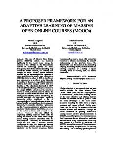
Percentage(%)
Urban distribution of miles & VMT 30 25 20 15 10 5 0 Interstate
Other Freeway & expressway
Other Principal Arterials
Minor Arterial
Collector
Local
VMT(%)
15.4
7
15.2
12.3
5.5
8.6
Miles (%)
0.4
0.3
1.5
2.5
2.6
17.7
Figure 2.3. Urban distribution of miles and VMT (Source: FHWA 2006) FHWA has identified five broad categories of road conditions, “poor”, “mediocre”, ”fair”, “good” and “very good”. "Poor" roads are considered to be in need of immediate improvement works. "Mediocre" roads refer to those that will sustain some kind of improvement in the near future in order to preserve usability. "Fair" roads pertain to the category of roads that will likely need some kind of improvement. "Good" roads are in decent condition and will not require any improvements whatsoever in the near future. "Very good"
14 roads have new or almost-new pavement and again will require no upgrading or repair works (FHWA 1999). Substandard road conditions can be extremely dangerous. Outdated and substandard road and bridge designs, pavement conditions, and safety features are accountable for 30% of all fatal highway accidents, according to FHWA. On average, more than 43,000 fatalities occur on the nation's roadways every year. Motor vehicle crashes cost U.S. citizens $230 billion per year, or $819 for each resident for medical costs and as a result triggers the following financial losses; lost in productivity; travel delays; and workplace, insurance as well as legal costs (FHWA 2006). Americans' personal and commercial highway travel continues to increase at a faster rate than highway capacity, and consequently highways can no more adequately support the current or projected travel demands. Between 1970 and 2002, passenger travel has doubled and road usage is expected to increase by nearly two-thirds in the coming 20 years. Growth can be attributed to changes in the labor force, income, makeup of metropolitan areas and other factors. More than 67% of peak-hour traffic occurs in congested conditions. The cost to the economy--in wasted time and fuel--in the 85 largest urban areas is $63.2 billion each year. In addition, poor highway conditions hinder the effective transportation of goods that help support the American economy (ASCE 2005).
2.2.2 Deterioration of transportation assets Transportation infrastructures cannot be completely protected from deterioration due to usage, climatic effects, or geological conditions. Furthermore, because of inadequate funding or inappropriate support technologies, certain components of this infrastructure have been neglected and have received only remedial treatments (Level 1996; National Research Council (NRC) 1996). According to the Board on Infrastructure and the Constructed Environment (BICE) (1999),”The United States spends an enormous amount of money
15 annually to replace or repair deteriorated equipment, machines and other components of the infrastructure. In the next several decades, a significant percentage of the country’s transportation, communications, environmental, and power system infrastructure, as well as public buildings and facilities, will have to be renewed or replaced.” This statement clearly depicts that the U.S. is no more in the so-called building era implying that it is more in the maintenance and management era, whereby proper maintenance is foreseen to foster the facilities’ proper functioning beyond the expected lifespan.
2.2.3 Funding limitations Currently, the U.S. is incapable of maintaining, even the present substandard, road conditions. Such inabilities are direct threats to both highway safety and the economy. As the nation's highway users await ratification of long-term legislation, America continues to lack the required funding for repairing roads and bridges which are categorized within “mediocre” state conditions (FHWA 2006). Not engaging in such endeavors greatly impede on the quality of life. Traffic congestion is costing the economy some $67.5 billion annually, which accounts for lost in productivity as well as wasted fuel (ASCE 2005). Unfortunately, passenger and commercial travel on highways has continued to augment spectacularly. The American Association of State Highway and Transportation Officials (AASHTO 1999) has estimated the capital expenditure by all levels of government to increase by 42% to arrive at the projected $92 billion cost-to-maintain level, and by 94% to attain the $125.6 billion costto-improve level. In disparity, the Federal Highway Administration has predicted that the outlay by all levels of government will have to be increased by 17.5% to reach its projected $75.9 billion cost-to-maintain level, and 65.3% to achieve its $106.9 billion cost-to-improve level. In 2000, the total capital investment by all levels of government was $64.6 billion, short of $106.9 billion desirable to enliven the system (AASHTO 1999).
16 In 1998, the endorsement of the Transportation Equity Act for the 21st Century (TEA-21), provided $218 billion for the nation's highway and transit programs. Even with this kind of investment, 33% of America's urban and rural roads still remained at substandard levels. Driving on defective roads cost U.S. motorists $54 billion per year in extra vehicle repairs and operating costs of $275 per motorist (AASHTO 1999). In 2003, an attempt made by the House Transportation & Infrastructure Committee, based on the investment requirements addressed by the FHWA’s 2002 report to congress, to introduce a legislation that would result in an investment of $375 billion in state highway and transit improvement programs over the six-year period (2004-09) failed lamentably. The problem of the nation's crumbling infrastructure is one of gargantuan proportions and if not addressed in the very near future it will likely pose a threat not only to public safety and welfare but also to the nation's growth and competitiveness.
2.3 Asset Management Overview Highways, as described in the previous section, will in time start to degrade and will require some kind of maintenance or repair in order to sustain its usability over its lifespan. The discipline that deals with such maintenance and repair works is termed asset management and the current section gives an overview of this specific field of study.
2.3.1 Definition of asset Any constructed facility can be considered an asset or an investment that needs to be maintained to ensure its most advantageous value over its life cycle. In the current research work the assets of interest are the highway pavements. Maintenance, as per British Standard 3811, is defined as ‘‘the combination of all technical and administrative actions
17 intended to retain an item in, or restore it to, a state in which it can perform its required function’’ (BS3811 1984). Various agencies have come to understand the critical importance of asset management (AM) and the followings are some of the “working” definitions adopted for AM.
“…a methodology needed by those who are responsible for efficiently allocating generally insufficient funds amongst valid and competing needs.” (Danylo et al. 1998)
“…a comprehensive and structured approach to the long-term management of assets as tools for the efficient and effective delivery of community benefits.” (Austroads 1997)
“Asset Management…goes beyond the traditional management practice of examining singular systems within the road networks, i.e., pavements, bridges, etc., and looks at the universal system of a network of roads and all of its components to allow comprehensive management of limited resources. Through proper asset management, governments can improve program and infrastructure quality, increase information accessibility and use, enhance and sharpen decision-making, make more effective investments and decrease overall costs, including the social and economic impacts of road crashes.” (OECDWG 1999)
“In the transportation world, asset management is defined as a systematic process of operating, maintaining, and upgrading transportation assets cost-effectively. It combines engineering and mathematical analyses with sound business practice and economic theory. The total asset management concept expands the scope of conventional infrastructure management systems by addressing the human element and other support assets as well as the physical plant (e.g., highway, transit systems, airports, etc.). Asset management
18 systems are goal driven and, like the traditional planning process, include components for data collection, strategy evaluation, program development, and feedback. The asset management model explicitly addresses integration of decisions made across all program areas. Its purpose is simple—to maximize benefits of a transportation program to its customers and users, based on well-defined goals and with available resources.” (Blueprint for Developing and Implementing an Asset Management System, Asset Management Task Force, New York State Department of Transportation, April 22, 1998).
All the above definitions ultimately boil down to defining asset management as a business process and/or a decision-making framework that provides a solid base on which agencies may rely in order to monitor and optimize the preservation, upgrading and timely replacement of assets through cost-effective management, programming and resource allocation decisions.
2.3.2 The Asset Manager’s dilemma Decisions about capacity expansion, maintenance/rehabilitation, and regular maintenance have been based merely on experience or perceived urgency of asset’s failure. Highway services are not being provided at an appropriate level and as a direct consequence these infrastructures are alleged to be aging faster than envisaged. Owners are accumulating an ever-increasing maintenance deficit, which in turn is leading to premature failures and premature renewals. Indeed, although the US federal agencies are investing on maintenance and renewal, the funds are never sufficient as the candidates requiring repair/maintenance are too much. Numerous reports have emphasized on the fact that many infrastructures are run inefficiently due to poor monitoring and control systems, water and road networks are deteriorating faster than anticipated, and the overall condition of US
19 bridges and pavements still remains gloomy (ASCE 2005; FHWA 2006). A lack of knowledge about the condition of the built environment means that the scarce resources that are available for maintenance and repair are often used inefficiently or inappropriately (Level 1996). These challenges affect everyone through increased health and safety risks, reduced economic competitiveness, inefficient maintenance strategies, reduction in the value of a nation’s built assets, and need to increase funding in order to maintain the built environment (ASCE 2005). In some cases, this overall inefficiency triggers the need for ‘‘new’’ buildings and engineering works, even when suitable facilities already exist or can be modified. Asset managers are human resources responsible for managing these substantial maintenance, repair, and renewal works (Vanier 2000). It is their prime and foremost responsibility to optimize expenditures and maximize the value of assets over the assets’ life cycles. In addition, asset managers are faced with many difficult decisions regarding how and when to repair their existing building stock cost-effectively and they have few effective and efficient tools at hand to assist them in the decision-making process (GAO 1998).
2.3.3 Asset management stages, tools and limitations The whole asset management framework can be divided into six broad stages and is in no way limited to highway asset management but may be applied to other fields such as building asset management amongst others. The different stages are described in the subsequent subsections; the tools utilized for each stage are enumerated with their salient limitations put forward.
2.3.3.1 Stage I - Inventory The first stage in any asset management tools, systems or models is the inventory modules, which are utilized to keep accurate track of the agency’s asset management portfolio.
20 Numerous systems exist, amongst which geographical information systems (GIS), computer-aided design (CAD) systems, and relational database management systems are some of the most employed. In GIS, data are directly related to their physical location on a map of the city or region. Current trend in the present stage seems to be more focused on the integration of satellite imagery data with GIS systems but however the main encumbrance appears to be the implementation phase (Vanier 2000). A very critical factor that has always been a major shortcoming for the use of the most up-to-date technologies is cost and as a consequence many agencies such as municipal and regional governments are financially in the incapacity of keeping up with such technological shifts (Oppman 1998). CAD systems are yet another credible source of asset management information for the engineering, technical, and management staff (Sommerhoff 1999). Dimensional information, such as areas and lengths, can be extracted from as built CAD drawings, which provide upto-date information about the extent of the assortment. However, mismatched issues with data formats (Vanier 1998 a. and b.) from CAD and CAD facilities management (CADFM) systems have often been questioned, especially if they are to be used for asset management. Another instrument that can be used to document the assets owned is the computerized maintenance management system (CMMS). There is a large selection of ‘‘fully commercialized’’ CMMSs available on the market, many of which are relational database applications that can be tailored to meet the data handling needs of asset managers (Vanier 2000). CMMS domains, at this time, are considered mature and stable, comprehensive, and useful tools proficient in administering work orders, trouble calls, equipment cribs, stores inventories, and preventive maintenance schedules. It should also be noted that many of these tools include numerous features such as time recording, inventory control, and invoicing. The CMMSs’ capability to store inventory data is formidable; however, their capacity with respect to life-cycle cost (LCC), service-life prediction, and risk analysis is
21 considerably less sophisticated. Such models are presently not able to assist the asset manager in analyzing data or scenarios for long-term system readiness, capability, or performance but nevertheless, CMMS are still considered to be an essential tool for the asset manager (Vanier 2001).
2.3.3.2 Stage II – Asset Worth Next to the inventory is the appraisal of the worth or net value of the assets. Six ways have been described in literature about the way to tackle this issue. Historical cost, also known as the original ‘‘book value’’ of the asset, is the first one. Second is the appreciated historical cost of an asset described as the historical cost calculated in present day dollars, taking into account annual inflation and/or deflation. Third, is the current replacement value, which depicts the cost of replacing the asset today. ‘‘Performance in use’’ value is the prescribed value of the actual asset (Lemer 1998), deprival cost is ‘‘the cost avoided as a result of having control of an asset’’ (ANAO 1996). Finally, market value, the value of the asset if it were sold on the open market today, is yet another way to go by determining the cost. This specific stage of asset management is deemed to be neither simple nor straightforward. Practice of large organizations is to store the historical cost of assets and to bring this cost forward to present day dollars using well-known building economic principles (ASTM E 917 1994) or to calculate the replacement cost based on the area, volume, or length of a system or component. Such endeavors do not present them with the ‘‘worth’’ of that asset but only the cost. Numerous ‘‘off-the-shelf’’ commercial tools such as the Building Life-Cycle Cost program (NIST 1995) have been developed to implement the above-mentioned ASTM standards. However, it is reported that practitioners do not make efficient use of these wellestablished LCC tools (McElroy 1999). Except for these types of LCC tools, there is little to
22 aid the asset manager in establishing the actual value of an asset and none of the available systems are comprehensive enough to save all six above-mentioned types of asset values.
2.3.3.3 Stage III – Deferred maintenance In this particular stage the emphasis is mainly on gauging the cost of pushing maintenance to some other point in time. Deferred maintenance can be taken as the accumulation of annual maintenance deficits, compounded from one year to the other (Vanier 2000). The compounding effect is analogous to the interest on a debt, implying that if maintenance is not concluded in the first year, then the costs of maintenance, repair, or replacement are higher in subsequent years. The “Law of Fives” is a very good approximation of this compounding effect of deferred maintenance. According to the law, not performing maintenance will result in repair works equivalent to five times the maintenance cost. In turn, not performing the repair works will later require renewal costs that can escalate up to five times the repair cost (De Sitter 1984).
Delaying maintenance amasses the amount of
deferred maintenance. From the asset manager’s standpoint, the rule of thumb with respect to the allocation of maintenance and repair funding is to cater for those assets in greater needs first.
2.3.3.4 Stage IV – Asset Conditions Conditions of assets are evaluated in this stage of the asset management framework. Numerous metrics exists amongst which facility condition index (FCI), condition index (CI) and condition assessment surveys (CAS) are amongst those mostly referenced in literature. The FCI is basically a ratio that compares deferred maintenance cost to current replacement value (CRV), which is the value required to rebuild the whole asset (Managing 1991; Kaiser 1996). Assets, with FCI greater than 0.15, are considered problematic. Technical condition
23 indexes (CI) as those implemented by the U.S. Army Corps of Engineers are yet another means of evaluating the conditions of assets (Bailey et al. 1989; Shahin 1992). The U.S. Army Construction Engineering Research Laboratory has pioneered the use of engineered management systems (EMS) in many construction sectors, including paving, roofing, and rail maintenance (‘‘EMS’’ 1998). The EMS assigns a condition index (CI) to an asset based on a number of factors including the number of defects, physical condition, and quality of materials as well as workmanship. These EMSs can, based on the data at hand, forecast the future CI, given the current state and a likely degradation curve. A number of systems exist for municipal infrastructure including PAVER (Shahin 1992), ROOFER (Bailey et al. 1989), BUILDER (‘‘BUILDER’’ 1998), and RAILER (‘‘RAILER’’ 1998). Condition assessment surveys (CAS) is another important decision-support tool used to evaluate existing condition of an asset. This tool in particular produces a yardstick for comparing different assets, as well as for the same asset at different times (BRB 1994; IRC 1994). Some of the potential applications of this system include: •
Assemblage of basic planning elements such as deficiency-based repair, replacement costs, projection of remaining life and the planning of future use.
•
Saving deficiencies of assets, the extent of the defect, as well as the repair work urgency.
•
Estimation of the cost of repair at the time of inspection.
Such tools enable asset managers to be in a better position to develop better optimal plans as regards maintenance and repair works (Coullahan and Siegfried 1996).
2.3.3.5 Stage V – Asset remaining life Next the remaining service life of the assets needs to be calculated. This is a step towards the determination of the life cycle cost for the maintenance, repair, and/or renewal
24 strategies. Tools and techniques utilized for such purposes include EMS as well as mathematical models such as Markov chain (Lounis et al. 1998). Since these means and methods of forecasting remaining assets’ service lifespan rely totally on studies of similar construction forms under test conditions, they regrettably require extensive data. However it must be noted that service-life prediction techniques are considered reliable within the bridge (Frangopol et al. 1997), pavement (Shahin 1992), and roofing asset management fields (Bailey et al. 1989; Lounis et al. 1998).
2.3.3.6 Stage VI – Decision making This last stage of the asset management framework is all about taking the most appropriate decision regarding which asset or assets will be the first to be allocated the necessary funds for maintenance, repair or renewal works. Such a task is not an easy one as there might be factors that are non-engineering into play, for example the decision makers’ preferences and risk attitude in asset management rendering the task very complex (Vanier 2000). Many researchers have been working on new decision making methodology that takes into account such complexity. Zhao et al. (2004) were able to produce a multistage stochastic decision-making model that accounted for the evolution of three uncertainties, namely, traffic demand, land price, and highway deterioration, as well as their interdependence. Gharaibeh et al. (2006) produced a decision making methodology that utilizes the complex multiattribute utility theory to assess the decision maker’s attitude toward the risk of infrastructure failure or inadequate performance. It is a known fact that the decision making process is embedded with multiple uncertainties due to political, social, and environmental interferences. In many of the asset management systems, decisions regarding maintenance and repair are made based on the assumption that the asset adheres to a perfect deterioration model, but
25 what if the deterioration model was not portraying real life deterioration mechanism. To address the problem, Durango-Cohen (2004) introduced the temporal-difference (TD) learning methods, a class of reinforcement learning methods, as an approach to maintenance and repair decision making for infrastructure facilities. TD learning methods do not require a model of deterioration and, therefore, can be used to address the above concern. Undeniably decision making is a major concern in all asset management tools and is continually soliciting a lot of attention from researchers, who are trying their level best to produce methods that can tackle this delicate yet complex issue.
2.3.4 Evolution of Asset Management and its tools In the earlier days, the mindset of owner of assets had a major role to play in its maintenance. These asset owners were more interested in building new assets rather than in maintaining those in need. Prior to the 1950s there existed only maintenance and no management. During that epoch, transportation projects, for instance, were maintained or developed based on intuition, personal experience, resource availability, and political considerations (Shahin 1992). Success of such ventures was often measured against the amount of control exerted on the backlog and not on the optimization of the system’s performance (FHWA 1999). Apart from the management strategy, other plausible reasons for such limited attention to maintenance could be attributed to the fact that during that period the transportation assets were not that consequent as it is today implying less competition for securing maintenance funding and also the technological tools at hand were scarce and very limited in application compelling the engineer to take matter in hands as regards to deciding on which asset to remedy first (Shahin 1992). After the 1980s, with the technological revolution of computers, automated data collection, testing equipment, design procedures, analytical tools and highway construction boom,
26 considerable progress was witnessed in the planning and programming arena of system preservation, upgrading, and operation. This laterally gave birth to a new discipline, asset management, which not only aided managers of assets in taking maintenance decision but also helped in the management of the system’s performance. During its initial development stages, AM was considered to be a very fragmented discipline, mainly attributed to a proliferation of software tools (Vanier 2001). At that point in time the numerous stand-alone systems had the abilities of solving myriad of problems relating to areas such as asset inventory, condition assessment, and strategic planning amongst others individually. Authorities involved with asset management had to own and operate several systems in order to make the right decision regarding which management and/or maintenance strategies are appropriate, making at the same time the whole process very tedious and time consuming. One of the main reasons attributed to such lengthy process was that the data manipulation from one system to another. Another crucial issue deplored was the fact that usage of different formats and databases gave rise to pools of unstructured data with poor interoperability (Kyle et al. 2000; Peters and Meissner 1995). Developers in this field have learned from their past misadventures and it seems that they have changed orientation in the sense that now more focus is laid on producing tools that are firstly capable of accepting input from a wide variety of asset management systems (interoperability characteristics are being inculcated into new systems) and secondly they are putting in their efforts to produce more integrated platforms. So far whatever has been described as regards to asset management can be applied to any discipline but since the current research interest is more oriented towards highways as transportation assets, the following section is dedicated to latter.
27
2.3.5 Highway Asset Management Highway agencies, such as the department of transportation, are continually investing large sums of money to maintain the physical and operational quality of their infrastructure assets above minimum levels. A highway infrastructure network consists of many components that are normally owned and managed by the same agency (e.g., pavements, bridges, culverts, signs, intersections, and guardrails). Managing these different components in a coordinated manner triggers benefits to both users and owners. Highway infrastructure management is the process of maintaining, rehabilitating, and reconstructing/replacing highway assets in a cost-effective way. For such endeavors, the highway agencies need tools that would enable synchronized management, repair and maintenance of their assets within the funding limits. In many highway agencies the use of separate management systems, as described in previous sections, are often incompatible in terms of location referencing systems, analytical procedures, and data input/output format. Thus, data sharing and communication among these systems become impractical and expensive. Present highway asset management systems are more centered on the analytical tool being utilized in the decision making process. Previous, older systems used only engineering principles and concepts but now the process also incorporates economic as well as behavioral models within its internal structure. This has given rise to more intelligent systems that allows competing investment options to be prioritized according to relative economic efficiency levels and at the same time providing a means of communicating the importance of transportation investments to the public and decision makers. Highway Economic Requirement System (HERS-state version), a highway asset management tool, has lately been much in the news. The HERS software was developed by FHWA in the mid-1990s. The software simulates the effects of future highway improvements
28 by comparing the relative benefit and cost associated with alternative improvement options on the basis of information about existing highways (FHWA, 2002). It begins by assessing the current condition of highway segments and then projects the future condition and performance in terms of congestion of the highway segments based on expected changes in traffic, pavement condition, and average speed. For each segment identified as deficient according to FHWA deficiency criteria, the model assesses the relative benefit and cost associated with improvement options to determine whether improving the segment is economically justified. The cost calculated includes improvement expenditure, and the benefit is computed as reductions in vehicle operating cost, travel time, and accidents over the service life of the improvement (FHWA 2002). This system is soliciting a lot of attention from FHWA, whose intention seems to make all the states in the US use the same highway asset management system. The system is continually being tested and updated based on feedbacks gathered from current users. It is important to note that inclusion of economic benefit gauging parameters into the system is making the system more credible and so far only a few of these economic parameters have been considered. This current study will be investigating other possible economic parameters of relative importance to highway investment projects and will be producing framework(s) that will show how the concepts would be integrated into the system.
2.4 Summary/Literature review In this chapter the deplorable conditions of the current U.S. transportation system was deplored and at the same time inferring that the building era is more than over. The current epoch is primarily dedicated to maintenance and management of the prevailing road system. The current status showed that the number of defective assets is accumulating from year to year due to unavailability of adequate financial support. The second section focused
29 more on what asset management is all about. The overall framework and the different stages involved in the decision making process were discussed emphasizing on the different tools and their limitations. Current development in the highway asset management systems appeared to be the inclusion of economic parameters into their internal structure in a quest to justify every penny being invested on the concerned highway improvement project. The next chapter will focus and review the different economic benefits associated with development projects.
30
CHAPTER 3. ECONOMIC BENEFITS
3.1 Introduction In this chapter the economic benefits associated with highway transportation projects are identified and described. The first section explains the numerous relationships existing between transportation investment and economic development, business location, productivity/output gains, production cost, and employment and economic growths. Furthermore the different categories of economic impacts as well as the measures used to gauge them are discussed. This section is concluded with the way this research work will be tackling economic benefits associated with highway maintenance and renewal projects. The second section describes the criteria for selecting the economic analysis tools as well as the final list of chosen systems that will be reviewed.
3.2 Existing relationships between economic benefits and highway investment. This specific section describes the existing relationships between economic development and highway transportation investment, pinpointing the economic impacts engendered, the measures used to gauge the transportation triggered economic benefits and lastly cautions about the benefits to be expected with transportation improvement ventures.
3.2.1 Highway infrastructure/economic development relationship The very complex and peculiar relationship between highway transportation and economic development has always intrigued researchers. Studies investigating the latter can be traced back to the 1960s, at which point in time the main focus was determined to be solely on economic and demographic changes incurred from the construction of a section of interstate
31 highways (Gkritza 2006). As from the 1980s, investigators were more fascinated in trying to discover any plausible evidence that would prove any existing link between highway transportation and economic development, and not simply economic changes. The outcomes of these investigations were mixed and more often incongruent. Nijkamp (1986), by using cluster and scaling methods and a quasi-production function, developed a multidimensional typological analysis of regional development in the Netherlands in the 1970s concluding that transportation infrastructure is a crucial determinant of regional output for both urban and rural areas. Aschauer (1989) showed through his research that public infrastructure has a positive impact on both investment and employment growth. Forkenbrock et al. (1990) examined different modes of transportation in the context of rural development and argued that highways are necessary but not sufficient for economic growth and development. However in the 1990s, practically all the studies carried out though using a myriad of methods, proclaimed the very existence of significant growth impacts (Quinet and Vickerman 2004) putting forward that changes in major highway system trigger changes in both local and regional economies (Baird and Lipsman 1990). More recent investigations have concluded that investment in transportation projects raises the long-term rate of economic growth (Jacoby 1999). It is undeniable that the recognized link between transportation and economic development is continually soliciting consequent public outlays in transportation systems at all levels (local, state and federal echelons).
3.2.2 Transportation infrastructure/Business location relationship Creation of new businesses or expansions of existing ones are dependent upon the quantity and quality of the surrounding infrastructures. Many studies have looked at how the location of highways affects a firm’s decision making process. Bartik (1985) made use of a conditional logit regression model to prove that the number of road miles is a significant
32 factor that impacts on the location of new manufacturing plants. According to McQuaid et al. (2004) transportation plays a deterministic role in establishing business locations by pondering on financial related issues such as the goods’ transportation costs, relative time and cost savings, certainty and reliability of travel time as well as on the staff and customer travel time and costs. Highway investment is considered most beneficial to businesses which have all the business related ingredients such as cost-effective labor, natural resources amongst others but no proper transportation access (Forkenbrock and Foster 1996). Based on numerous recent and past research works, it can be asserted that a new transportation facility in a business region does not necessarily generate economic success but however is a vital foundation to improving the current existing conditions (Hodge et al. 2003).
3.2.3 Transportation infrastructure/ Productivity-Output relationship. Based on the theory of production, economists were able to mount up a production equation which used labor, public infrastructure and human capital as inputs. The outputs were measured using the gross state product (GSP), private GSP and/or manufacturing output. The noted outcome was that an increase in the highway stocks triggered an increase in the output (Munnell and Cook 1990b; Eisner 1991; Coughlin et al. 1991; Conrad and Seitz 1994; Moonmaw et al. 1995; Crihfield and Panggabean 1995; Boarnet 1996; Garcia-Mila, McGuire, and Porter 1996; Harmatuck 1996; Boarnet 1998; RESI 1998; Fernald 1999). Whatever be the level at which the output is being gauged, it seems that the result is still positive. For example, 1% increase in highway stock annually will increase the output by 0.35% at national level (Fernald 1999). Another study carried out at state level, Maryland, showed that a 1% increase in the annual highway stock resulted in an increase in the output by 0.06% (RESI 1998). Furthermore at county level the trend is still unaltered, improvements
33 in county’s highway stock significantly improve economic benefits (Boarnet 1996). Transportation improvements generate a series of productivity gains that can hamper on how businesses functions (AASHTO 1999). Businesses will continually undergo changes in response to improvements in infrastructures in a quest to improve current labor productivity. In general, efficiency improvements result in a decrease in the agency’s costs and an increase in the company’s profit levels (Gkritza 2006).
3.2.4 Transportation infrastructure/Production costs relationship. The relationship between public investments and production cost was found to be negative and statistically significant (Berndt and Hansson 1992; Lynde and Richmond 1993; Seitz 1993; Nadiri and Mamuneas 1994; Conrad and Seitz 1994; Morrison and Schwartz 1996; Holleyman 1996; Harmatuck 1996; RESI 1998). The derived narrow range of -0.05 to +0.21 percent reduction in production resulting from a 1 percent increase in the stock of transportation infrastructure seems to bring some credibility to the used models. These cost models were used at different levels, national (Berndt and Hansson 1992; Lynde and Richmond 1993; Seitz 1993; Nadiri and Mamuneas 1994; Conrad and Seitz 1994; Holleyman 1996), states level (Morrison and Schwartz 1996a, 1996b) and even at a single state level (RESI 1998). Disaggregation to a microscopic level by splitting the economy into different types of industries showed that the impact of such investments vary with the type of industry but will range between -0.11 to -0.21 inferring that the benefits derived is industry dependent (Nadiri and Mamuneas 1994). Thus, transportation infrastructure plays a crucial role in reducing the production costs of industries. Furthermore as these infrastructures are improved, a net decrease in the distribution costs is witnessed with an improvement in the firms’ accessibility to the labor market. A study performed by the office of the federal highway administration back in 1993 on the relationship between highway transportation
34 and the productivity of industries indicated that the expected rate of return to the manufacturing sector, as a whole, within the first year is 6.6 percent (Gkritza 2006). Highway investment is also a significant factor in long-term changes production technologies and processes. An increase in highway capital has been found to result in a drop in the demand for labor and materials (demand cross-elasticities of –0.02 and –0.01, respectively) by enabling production reductions in locations where these inputs are less efficient. However, these increases in productive efficiency can also stimulate the demand for private capital as a substitute for labor. Increases in private capital investment can subsequently lead to business expansions and economic growth (Jacoby 1999).
3.2.5 Transportation infrastructure/Employment and Economic growth relationship. Practically all the studies carried out on this particular measure are categorical on the outcome; a positive and significant relationship exists between capital investments and economic benefits (Aschauer 1989c; Jones 1990; Mofidi and Stone 1990; Duffy-Deno and Eberts 1991; Coughlin et al. 1991; Luce 1994; Singletary et al. 1995; Bruinsma et al. 1997; Haughwout 1999). One of the interesting aspects of these studies was that they focused on different spatial units such as states, metropolitan areas, local governments or small zones. One such study even used micro data on individual housing values, central city and suburb to gauge the benefits (Haughwout 1999). When within a particular region the unemployment, per capita income, and poverty levels relative to the state or adjacent regional levels are so low indicating that the region’s economy is chaotic or depressed, then in order to remedy the economic situation very often transportation investment are sought. Such endeavor is regarded as a means of bringing some competitiveness to the region implying at the same time that highways are positively related to employment and income
35 growth. However the relationship’s strength is weaker for rural compared to urban areas, as well as for non-metropolitan areas compared to metropolitan areas (Brown, 1999). During the 1970s, employment and population densities were positively affected by the presence of limited access highways and the study by Carlino et al. (1987) showed that it was the interstate highway program that is the main reason behind the redistribution of population and employment in the US, although it was not the main intent of the program. Deno (1988) agreed that public capital plays an important role in manufacturing firms’ output supply and input demand decisions. Empirical analysis suggests that highway investment has a significant effect on regional output, especially in declining regions (Gkritza 2006).
3.3 Economic impacts linked to transportation projects Though the relationship between transportation investment and economic growth is a very complex, yet this causal relationship may be broken down into three main categories, namely: (1) differences in highway effects occurring over time, (2) differences in highway effects by industry, and (3) differences in highway effects by region. Researchers when undertaking investigations on temporal impacts on highway typically divide the study period into construction (short-term) and post-construction stages (medium- and long-term) (Gkritza, 2006). During the construction period, a region is recognized to experience an exogenous boost in construction expenditures, which is nonstop over a few years basically until the project is completed. During the post-construction phase, the construction stimulus is removed making economic effects more difficult to assess. Most studies have cramped their evaluation periods to two decades after construction or less. One view is that the effects are immediate; another view is that they are realized after a lag of several years. Lags between four and seven years have been estimated empirically (Rephann and
36 Isserman 1994). In the long-run, what actually happens depends on the relative scarcity of land, labor and capital (Flyvbjerg et al. 2003). Apart from the economic impacts of highway investment related with the different phases of a project, the relative maturity of the transportation system also needs due attention. Implanting a new highway infrastructure into a less developed transportation system area will have a larger impact than a highway project introduced into an area with a mature system (CUBRC et al., 2001; Nadiri and Mamuneas 1998). Highway infrastructure investments made during the 1950s through the 1970s had a larger economic impact than those made in the 1980s with the decrease attributed to the highway network becoming more comprehensive and dense in its coverage. Research works carried on returns on highway investment have noted decreases over time (Mamuneas and Nadiri 1998). Furthermore, the distribution of highway effects also varies by industry. Most industry research focuses on three sectors: manufacturing, retail trade, and services (Rephann and Isserman 1994). Most information is available on how location decisions work for the manufacturing sector, whereas little is known about the other industries. Finally, the potential for secondary effects, and thus the need to conduct specific analyses to determine the possibility of impacts also depends upon the type of project being proposed. Capacity improvements, additional interchanges and construction on new location generally have a greater potential for indirect effects than projects to upgrade existing facilities (FHWA 1992). As such, it is recognized that the economic impact of any particular project is still best evaluated on a case-by-case basis (McQuaid et al. 2004). However, questions remain as to how differing types of highway investment affect economic development. In conclusion the four broad categories of economic impacts consequential to investment in transportation projects are, direct, indirect, induced, and dynamic economic impacts (Forkenbrock and Weisbrod 2001) and are briefly described next.
37 Direct Economic Impacts Short-run or direct benefits are the employment, earnings, and spending stimuli that spread from the construction industry to suppliers, workers, and retailers. Multipliers from inputoutput tables are used to estimate the industry-by-industry effects of a transportation project (Gkritza 2006). For illustration, if an owner invests one billion in a highway project, the yield as regards to employment and income effects would roughly be similar as one billion dollars spent in another construction project as the short-term economic benefits are not unique to public transportation (Bhatta and Drennan 2003). Indirect Economic Impacts Such benefits refer to the increased purchases by the direct beneficiaries of the investment, which for such investment may offer direct benefits to a manufacturing company within the region, but however indirect benefits is expected to be amassed by suppliers of the manufacturing company and the manufacturers’ employees through increased wages (Gkritza 2006). Boarnet (1996), in his working paper entitled “The Direct and Indirect Economic Effects of Transportation Infrastructure,” clearly pinpoints on the occurrences of both direct and indirect impacts. Direct effects basically referred to the economic impacts that occurred within the jurisdiction of the highway project while the indirect effects are foreseen to occur outside the highway implementation project’s jurisdiction. Most investigators used one or more of the following six measures to gauge the long term economic benefits; (1) output;
(2) productivity; (3) cost of production; (4) income, property
values, employment and real wages; (5) rate of return; and (6) non commercial time. Though different studies produce different numerical answers, yet the outcomes showed positive and statistically significant relationship between the investments and the gains (Bhatta and Drennan 2003).
38 Induced Economic Impacts The resulting increase in the wages of the people within the region will incite them to spend more leading to induced benefits by the businesses that provide food, clothing, and other consumer services (Gkritza 2006). Dynamic Economic Impacts These impacts are the long-term changes in population and business location patterns as well as the resulting land use changes, which will in turn affect income and wealth in the area (Gkritza 2006). The interrelationships between the four broad categories of economic impacts are depicted in Figure 3.1. If all the impacts illustrated in the above figure were to be summed then this would represent the total effect on economic growth. Dividing the total effect by the direct effect yields a ratio referred to as “economic multiplier” and likewise both the indirect and induced effects can be grouped together and the resulting effects referred to as “multiplier effects.” The above described economic multiplier is composed of output, employment and income multipliers, whose magnitude is dependent on the type of transportation investment and the size of the area economy. Typical output multipliers for most transportation ventures are in the range of 2.5 to 3.5 (national level), 2.0 to 2.5 (state level) and 1.5 to 2.0 (local level) (Weisbrod and Weisbrod 1997). If a $250 million highway improvement takes place along a corridor, it can be expected that the net impact on the total level of economic activity in the study area may be increased by $375–$500 million.
39
Dynamic Impacts Property values, Land use/development, Environment, Revenue and cost
Change in transportation system
Change in user costs Total Direct, Indirect & Induced Impacts
Change in Business
Regional Output, Gross Regional Product, Wages and Jobs
Costs & Markets
Direct Impacts
Indirect Impacts Change in Supply Purchases
Change in Business Activity of directly affected business
Induced Impacts
Change in Business activity of Suppliers
Change in ave. & total worker wages
Change in Business activity of Consumers
Change in Earnings retention
Figure 3.1. Interrelationship between economic impacts (Adapted from: Gkritza 2006)
3.3.1 Measures of economic impacts For measuring economic impacts linked to a transportation investment venture there exist a multitude of overlapping measures, which can be organized into the following four categories (Weisbrod and Weisbrod 1997) as illustrated in Table 3.1.
40 Table 3.1. Economic impact measures Category
Category-measure
Description
Category 1
User Impact
In order to determine the value of user impacts the components of the latter, such as money cost of travel, travel time, safety, and comfort/reliability are used and combining all result in total user impacts.
Category 2
Economic Impact
In this particular category, the following measures have been identified as,
•
Regional output;
•
Gross regional product (GRP) or value added;
•
Jobs;
•
Wages and other income;
•
Number of businesses;
•
Business volume and sales;
•
Population;
•
Private
investment
in
buildings,
plant,
and
equipment; and •
Real estate values (Weisbrod, 2000; EDRG and CSI, 2001).
Category 3
Category 4
Government
Fiscal
This
category
includes
public
revenue
and
public
Impacts
expenditures.
Other Societal Impacts
Include air quality, other environment conditions, and social conditions.
3.4 Economic benefits/highway maintenance and renewal projects It is important to point out that highway projects that are commonly dealt with by asset managing agencies are more of the maintenance and/or renewal types. However the above description about economic benefits is associated with basically new development projects
41 and in the literature there exist no such studies or investigations dealing with the impact of investment on highway maintenance or renewal projects. For this particular research venture, the types of economics benefits associated with highway maintenance, renewal as well as with completely new project ventures are considered to be similar. However, the magnitude of the different economic benefits associated with repair/maintenance projects is foreseen to be less than for new developments.
3.5 Selection of Highway Economic tools for review Now that the economic benefits associated with highway maintenance and renewal projects have been described, the next obvious step is to select some of these readily available systems for review in order to have a more in-depth understanding of the underlying economic concepts as well as their limitations. On the FHWA web site (http://www.fhwa.dot.gov/planning/toolbox/bibliography.htm#aashto, access date: 01/02/2008), there exists under the planning section a compilation of the bibliography of systems used in managing transportation assets. Some of the main criteria used in selecting the economic analysis tools for review are as illustrated in Table 3.2.
42 Table 3.2. Criteria used for selection of economic analysis tools. No.
Criteria description
1
Who is the owner/promoter of the system?
2
Type of software? a. Is it a freeware? (Preferred) b. User-friendliness of the system. c. PC requirements to install and run software.
3
Availability of documentations. a. Any technical manual? b. Any system user manual?
4
Who the users are? Preference is given to systems used by the department of transportation, which are the highway asset management agencies.
5
Is the system undergoing continuous enhancement and rigorous testing by concerned authorities?
Based on the above criteria, the selection was made, Table 3.3. Table 3.3. Selected Economic Analysis tools. No.
System
1
Highway Economic Requirement Systems – State Version (HERS-ST)
2
Surface Transportation Efficiency Analysis Model (STEAM)
3
California Life-Cycle Benefit/Cost Analysis Model (Cal-B/C)
4
Regional Input-Output Modeling System (RIMS II)
5
Impact Analyses and Planning (IMPLAN)
6
Regional Economic Modeling, Inc (REMI)
7
Transportation Economic Development Impact System (TREDIS)
43
3.6 Summary/Economic benefits In this chapter the different relationships existing between investment in transportation infrastructure and engendered economic benefits were identified and described. Studies gathered from the literature indicated that highway investment can be linked to economic development within and away from the project vicinity. Business location was also affected by the number as well as the quality of existing roads. Furthermore productivity gains, production costs and employment as well as economic growth were all influenced by transportation infrastructures. The identified relations produced four types of economic impacts, namely, direct, indirect, induced and dynamic. This research work will be more focused on direct and indirect economic benefits and will treat remedial highway investment as new development projects as regards to economic benefits generated. The last section considers the criteria used in the selection of the economic analysis tools and finally provides the complete list of the selected systems.
44
CHAPTER 4. ECONOMIC ANALYSIS TOOLS – REVIEW
4.1 Introduction This whole chapter reviews some of the different economic analysis systems, currently available on the market and specifically used in the management of transportation infrastructures. It is divided into three main parts. In the first part, clear distinction is made amongst the economic efficiency analysis tools and the economic development impact systems. Each of the identified system under each group is reviewed and the salient characteristics as regard to its purpose, composition and advantages are summarized. The second part is a compilation of the limitations associated with the different tools while the last part is all about the review matrix, a one sheet summary of the whole system reviewed.
4.2 Review of Economic Analysis tools This section is dedicated to the appraisal of the selected economic analysis tools. From the preselected list, two separate categories of tools have been identified. The first category has been termed economic efficiency tools and includes systems such as HERS-ST, STEAM 2.0 and Cal B/C, while the second group referred to as economic development tools includes the remaining tools identified in the previous chapter. The review presented in this chapter will be divided into the following three parts. The first one will describe the purpose of the system, part two will focus on its composition that is what are the main building blocks within the model’s internal structure and finally the last one will elaborate more on the benefits and advantages of using the system. The systems will be reviewed in the same order as it appears in Table 3.2.
45
4.2.1 Tools for Economic Efficiency Analysis The evaluation of transportation projects has traditionally been carried out in the context of economic efficiency in terms of savings in travel time, vehicle operating cost, and safety (Gkritza 2006). HERS-ST, STEAM 2.0 and Cal B/C are the economic efficiency tools reviewed and described next.
4.2.1.1 Highway Economic Requirements Systems – State Version (HERS-ST) The Highway Economic Requirements System (HERS) is a computer model designed for the Federal Highway Administration (FHWA) by Jack Faucett Associates (FHWA 2002). The software is capable of estimating benefits to highway users (travel time, operating costs, and safety), two types of benefits to highway agencies (maintenance costs and the “residual value” of an improvement at the end of the analysis/funding period), and one “external” benefit (reduction in vehicle emissions) from potential highway improvements projects. In short, it estimates the amount of finances required for injecting on highway improvement projects based on benefit-cost grounds. Deficiencies in the highway sections are computergenerated and identified through the utilization of engineering concepts while the selection of improvements for implementation is simulated based on applied microeconomic principles. FHWA utilizes output from the HERS model in preparation of the Department of Transportation’s (DOT) biennial “Status of the Nation’s Surface Transportation System • Condition and Performance • Report to Congress (C&P Report)”. The way the system functions is straightforward: (1) forecast section condition; (2) identify deficiencies and possible improvements; (3) appraise and choose improvements; and (4) implement improvements (or, for unimproved sections, implement the unimproved condition forecast for the end of the period). The complete HERS-ST process is schematically
46 illustrated in Figure 4.1. The Highway Performance Monitoring System (HPMS), an annually updated stratified random sample database of more than 100,000 sections of non-local roads statewide, is the principal data source of HERS-ST (FHWA 2002). For the system to kick-off, as will be the case with the other systems that will be under review, there must be at least two scenarios, a base case (do-nothing or less aggressive alternative) and an improvement one. The model utilizes the base-year of the highway system to predict changes to the system and consequently analyzes impending improvements for each of several “funding periods”, which can be specified by the user. As a rule of thumb, the funding periods are defined in multiples of 5 years and for each of them the output statistics are amassed and the process recurred (FHWA 2002). For each subsequent funding period, sample section and logical sequences, HERS-ST makes use of its inbuilt internal models (speed calculation, pavement wear, traffic forecasts, capacity calculations, and user, agency, and external costs models) to predict the same set of parameters; (1) Future trafic volume ;(2) Pavement conditions ; (3) Current and future speeds, and (4) Section capacity after improvement Based on the above predictions, again for each funding period, the software calculates three main cost classes: (1) Highway user costs (Operating costs, travel time costs and safety costs); (2) Agency costs (initial capital improvement costs and maintenance costs), and (3) External costs (societal costs associated with vehicle emissions),
47
For each section For each funding period Forecast Conditions
Identification of inexpensive mandatory Improvement
Reached mandatory funding constraint?
Yes
No For each section Select most attractive improvements to limit of reserved funds
Non-mandatory Funds Available?
Yes
Evaluation of more aggressive improvements
Pre-select most attractive improvement scenario
No
Select most attractive improvement to limit of total funds
Implement selected improvements
Figure 4.1. Schematic representation of HERS-ST logical sequence (FHWA 2002)
48 The final part of the process is the determination of the benefit-cost ratios of the different scenarios under consideration. Benefits are taken to be the cost reduction occurring as a result of an improvement, measured as the difference in costs between the base case and the improved one. On the other hand, disbenefits refer to the increase in costs as a consequence of a particular improvement. HERS-ST will typically implement the cases with benefit-cost ratios greater than 1 (FHWA 2002). Amongst the myriad capabilities of the system there exists the ability to predict the condition and performance of the State’s highway system over the next 20 years with scenarios depicting reduction or increase in the funding levels. Also the level of future investment required by a State’s highway system to ensure an average effective travel speeds on the system can also be answered by this tool. Furthermore, it gauges the level of financial support needed to make all economically beneficial improvements on the system. Last but not least, it can also be utilized to answer “What are reasonable performance targets given funding, policy, and customer satisfaction objectives?” In conclusion it can be said that the ultimate goal of HERS-ST is to optimize the rapport between public highway investment and user costs (FHWA 2002).
4.2.1.2 Surface Transportation Efficiency Analysis Model (STEAM) The enactment of the Intermodal Surface Transportation Efficiency Act has compelled planners to contemplate more on the evaluation of multimodal alternatives and demand management strategies. In 1995, FHWA developed the Sketch Planning Analysis Spreadsheet Model (SPASM), a corridor sketch planning tool to assist planners in comparing cross-modal and demand management strategies (DeCorla-Souza et al.1996). In 1997, FHWA introduced the Surface Transportation Efficiency Analysis Module (STEAM) for detailed, system-wide analysis of alternative transportation investments.
STEAM
49 became the first FHWA impact analysis product to use input directly from the four-step travel demand modeling process. The system uses benefit-cost analysis to contrast between the economic worth of alternatives, through the assessment of trade-offs between the mobility and safety benefits of transportation infrastructure projects, and the cost of building, maintaining and operating these projects. The current version, STEAM 2.0, is an updated version of STEAM containing many enhancements, such as, (1) specification of project capital costs in excess of $999 million; (2) specification of any discount rate; (3) network checking function; (4) bus market sector output; (5) re-use of travel time files previously generated; and (6) network skim function that greatly reduces processing time (DeCorlaSouza et al.1996). One of the significant features of the new version is its ability to report mobility and safety benefits by user-defined districts. The district reporting and accessibility features are new tools for gauging the social impacts of transportation investments. The district-level reporting allows users to contrast the impacts of transportation investments to resident trip-makers across aggregations of zones while the accessibility feature generates approximations of employment openings within the user-defined travel-time threshold of a district across a base and improvement scenario. Estimates and costs gauged by the model includes, (1) benefits and costs to transportation users, (2) annualized cost to public agencies, (3) effect on total transportation cost, (4) change in accessibility to jobs for district residents, (5) change in emissions for particulates, hydrocarbons, carbon monoxide, and nitrogen oxides, (6) change in energy use, (7) change in noise and other external costs, (8) change in fatal, injury, and property damage only accidents and (9) revenue transfers due to toll or fare changes (FHWA 2005; CSI 2000). The model uses the conventional four-step planning models to generate more accurate highway travel speeds under congested conditions. Unlike HERS-ST, STEAM 2.0 performs
50 risk analysis to describe the level of uncertainty in the results produced. The model furthermore is capable of developing monetized impact estimates for a wide range of transportation investments and policies, including major capital projects, pricing and travel demand management (TDM) to the extent feasible. Flexible in terms of transportation modes, trip purposes, and time periods analyzed it also has default analysis parameters for seven modes (auto, truck, carpool, local bus, express bus, light rail, and heavy rail) allowing the user to deal with special circumstances or new modes by modifying these parameters. System requires both a base Case and an Improvement Case trip tables for different trip purposes to kick off.
Regarding time periods, STEAM 2.0 can be applied to average
weekday traffic or to peak and off-peak traffic with different definitions of the peak periods. The modules and its functional description are illustrated in Figure 4.2, while the cost and benefit estimation models within its internal structure are as outlined below: 1. User benefits model, 2. Congestion analysis model, 3. Accident costs analysis model, 4. Emissions analysis model, 5. Fuel consumption analysis model, 6. External costs analysis model, 7. Capital costs model, 8. Revenue transfers model, 9. Accessibility analysis model, and 10. Risk analysis model.
51
User Interface Module 1. 2. 3. 4.
Specify Parameters Specify travel forecasting model files Specify optional district definitions Specify demographic data for optional accessibility analysis mode 5. Runs model 6. View results
STEAM SYSTEM MODULES
Network Analysis Module 1. Calculate highway link speeds 2. Calculate highway and zone to zone travel times and distances
Trip Table Analysis Module 1. Calculate user benefits using consumer surplus 2. Calculate highway emissions, energy use, noise costs amongst others
Evaluation Summary Module 1. Calculate annualized cost to transport agencies 2. Summarizes regional user benefits and external costs 3. Summarize district-level mobility and safety benefits 4. Summarize accessibility impacts by districts 5. Perform risk analysis
Figure 4.2. STEAM 2.0 system modules and function descriptions (CSI 2000)
52
4.2.1.3 California Life-Cycle Benefit/Cost Analysis Model (Cal-B/C) The California Life-Cycle Benefit/Cost Analysis Model (Cal-B/C) is used for the economic evaluation of potential highway and transit improvement projects within the state of California only. Issues handled with respect to highway projects include lane additions, high occupancy vehicles (HOV) lanes, and intersections amongst others. Transit modes readily considered by the system are inclusive of passenger rail, light rail, and bus. Cal-B/C is a very simple system (MS excel format spreadsheet) designed to measure the following four main categories of benefits resulting from the above-mentioned improvement projects, (1) travel time savings; (2) vehicle operating cost savings; (3) safety benefits (Accident Reductiom Cost Savings); and (4) emission reductions (Caltrans 2007). The system analyses the 20-year economic lifespan of the improvement project beginning after the startup phase, which varies between one to seven years. For kick-off the system requires annual transit person-trips and the representative annual average daily traffic for the highway facility under investigation for both the base case and the proposed improvement alternative. Inputs are factored to peak and off-peak volumes and (for highways) truck volumes. HOV lane volumes, if included, are entered separately. As needed, free-flow speeds, before-after transit trip times, transit vehicle-miles and beforeafter accident data are entered, along with fixed costs and annual costs, on a year-by-year basis (Caltrans 2007). The outputs, which are gauged over the lifespan of the project (assumed to be 20 years), are summarized on per-project basis using the following outlined measures: •
Life-cycle costs (in $ million)
•
Life-cycle benefits (in $ million)
•
Net present value (in $ million)
53 •
Benefit-cost ratio (benefits/costs)
•
Rate of return on investment (in % return/year)
•
Project pay back period (in years).
All the values and rates, specific to the state of California are already incorporated in CalB/C as defaults are shown in Table 4.1. Table 4.1. Values and rates provided by Cal-B/C system Parameter
Value/Rate
Real discount rate
6%
Value of time for Automobile
$8.16/hour
Truck
$27.72/hour
Transit passengers
$8.16/hour
This system is very efficient for usage in the state of California, principally because very little input data are required if the user making use of the built-in default values specific to that particular state. Otherwise these default values can easily be replaced (Caltrans 2007).
4.2.2 Tools for Economic Development Impacts Information on economic development effects of proposed highway investments is valuable for understanding the total impact of project proposals and ensuring an efficient allocation of resources (Gkritza 2006). The systems reviewed under this specific section have the same purpose that of evaluating economic development impacts.
54
4.2.2.1 Input-Output models Input-output (I-O) models are economic tools utilized in the evaluation of economic impacts of investments on the affected regions. I-O table, or Input-Output table, measures the goods that a particular industry buys from all of the other industries ("inputs"), which are also known as intermediate inputs. I-O values also include the goods purchased by the intermediate suppliers of the industry. The table can be read as inputs from (industry in row) purchased and converted to output by (industry in column). The values are proportions, so that for every $1 of output by the industry represented by column x, a certain number of cents worth of goods was purchased from each industry y, as given by the value in row y of column x. I-O table calculates the additional output or jobs that would be created by increasing output for a particular industry; thus, it captures the indirect and induced effects of shocking a specific industry or group of industries. These tools are considered to be very effective planning tools for public and private-sector projects at any level (national, state or local). Simply put, they simulate the inter-industry relationships within regions, which determine how regional economies are likely to respond to project changes (CSI and BLA 1998). Apart from the direct effects, these systems have the ability to capture the secondary indirect and induced effects (the effects of household spending). A wide range of such models are on the market, ranging from the relatively inexpensive and fairly simple U.S. Department of Commerce, Regional Input-Output Modeling System (RIMS II) to the reasonably priced and more complex Minnesota IMPLAN input-output model or choose the most sophisticated and expensive integrated input-output-econometric model developed by Regional Economic Modeling, Inc. known as REMI.
55
4.2.2.2 Regional Input-Output Modeling System (RIMS II) RIMS II is based on an accounting framework called the Input-Output (I-O) table, which shows the industrial distribution of inputs purchased and outputs sold for each industry. The model uses Bureau of Economic Analysis’s (BEA) national data sources (a compilation of nearly 500 U.S. industries) and BEA’s regional economic accounts to construct the required I-O table for any region as well as for any group of industries. Two possible I-O multiplier tables are possible: Series 1 (for 490 detailed industries), and series 2 (for 38 industry aggregations). Each series is composed of four tables: (1) final-demand output multipliers, (2) final-demand earnings multipliers, (3) final-demand employment multipliers, and (4) summary final-demand multipliers for output, earnings, and employment and direct-effect multipliers for earnings and employment (BEA 1992). RIMS II adopts a three-step process. The first step makes the producer portion region specific, the second one is a repetition of step on with emphasis on households. Finally the last step uses the Leontief inversion approach to measure output, earnings, and employment multipliers. RIMS II multipliers can be applied to projects only if the spending data are at hand, which should include industry category, year of expenditure (to determine the time period of the economic consequences and to adjust to 1997 dollars) and the spending location as multipliers are location specific. Results from the system are then expressed as earnings (wages and salaries), output (economic activity) and jobs (Lynch 2000).
4.2.2.3 IMPLAN Model IMPLAN is a non- survey based input-output system similar to REMI (discussed next). The acronym is for Impact Analyses and Planning. IMPLAN was originally developed by the U.S. Forest Service in cooperation with the Federal Emergency Management Agency and the
56 U.S. Department of the Interior's Bureau of Land Management to assist in land and resource management planning. Since 1993, the IMPLAN system has been developed under exclusive rights by the Minnesota IMPLAN Group, Inc. (Stillwater, Minnesota) which licenses and distributes the software to users. In 1995 MIG, Inc. started writing the new version of the IMPLAN software from scratch, which extended the previous Forest Service version by creating an entirely new modeling system that included Social Accounting Matrices (SAMs) – an extension of input-output that resulted in the generation of SAM multipliers. The IMPLAN model was designed for three purposes, namely, data retrieval, data reduction and model development, and impact analysis. Detailed data of the entire U.S. by county, and the ability of incorporating user-supplied data at each stage of model building, renders the system highly flexibility both in terms of geographic coverage and model formulation. Two major parts of the database are the national-level technology matrix and the estimates of sectorial activity for final demand, final payments, industry output, and employment by county, state and at national levels. The model produces multipliers for employment, output, value added, personal income, and total income (Lynch, 2000). County Business Patterns and BEA data are the main sources of employment and earnings data and estimates are made at state level. Some of the capabilities of the IMPLAN system include; (1) establishing the effects of a company moving into an area or the contributions of an existing company; (2) measuring industrial targeting opportunities; (3) observing resources regulated by the government; (4) analyzing benefits of commercial development and usage of such information to attract new companies; (5) measure the effects of the tourism industry; (6) examine a region's strengths and market opportunities; and (7) analyzing a wide variety of other economic/marketing issues (MIG 2006)
57
4.2.2.4 Regional Economic Modeling, Inc (REMI) REMI is considered to be an eclectic model linking both an input-output model to an econometric model. Turning the econometric module off suppresses the model to an inputoutput model. REMI is a dynamic model that captures impacts over time. The concept of regional equilibrium is central to the model's long-term portrait of regional economic growth. As such the model is made of five blocks: output, labor and capital demands, population and labor supply, wages, prices, and profits, and market shares (REMI 2007). The system requires extensive data from three sources of employment and wage and salary data: the Bureau of Economic Analysis (BEA) employment, wage, and personal income series (averages which are reported at the two-digit level for states and at the one-digit level for counties), ES-202 establishment employment and wage and salary data ( this is the foundation for BEA data, and are collected monthly in conjunction with the unemployment insurance program at the two-digit level for counties and states), and County Business Patterns (CBP) data published by the Bureau of the Census (data collected in conjunction with the Social Security program in March of each year). The REMI model is preferred over input-output modeling for long-range planning owing to its dynamic nature and its ability to account for productivity changes that may develop as a result of transportation decisions over a 20- to 30- year planning horizon (CUBRC et al. 2001; Forkenbrock and Weisbrod 2001).
4.2.2.5 Transportation Economic Development Impact System - TREDIS TREDIS is a web-based interactive system of tools owned by the Economic Development Research Group Incorporation. Specifically designed for transportation planners, TREDIS is capable of evaluating economic impacts of transport projects within all modes of freight and passenger travel such as cars, trucks, buses, passenger trains, freight trains, aviation and
58 marine means of transportations. Developed by economists, the system gauges the changes induced in productivity factors including the availability, breadth and activity level of ports/terminals, labor markets, building/site facilities, infrastructure and international trade by investments in transport infrastructures. The internal structure of system is based on recent advances in economics, “new economic geography”, and has inbuilt threshold effects related with changes in service areas, market access and travel times that permits direct and indirect impacts to be estimated. Direct effects such as travel-related cost changes and market access charges associated with a project are determined first, then follows the indirect effects engendered from inter-industry supplier-buyer linkages, as well as effects generated by the recirculation of wages into the local economy. Additional economic impacts are computed by using any one of the TREDIS linked models, namely, (a) CRIOIMPLAN model; (b) REDYN model; or (c) REMI Policy Insight model. As such the TREDIS system is made up of four independent modules as illustrated in Figure 4.3 (EDR 2007). Some of the main strengths and use of TREDIS include, (1) estimation of the economic impact of constructing a transportation terminal or facility; (2) estimation of different strategies for managing a transportation corridor; (3) performance of a comprehensive freight performance evaluation; (4) comparison of the benefits and costs of alternative transportation investment strategies or policies; (5) estimation of the impact of congestion on households and industries (by sector), based on their usage of different modes; and (6) systematical evaluation of the economic benefit of improving multimodal access to consumer, producer, and labor markets (EDR 2007). "Regional economic impacts" are distinguished from "benefit/cost accounting" by separating various elements of travel efficiency, cost savings, productivity and environmental impacts to portray benefits from the differing perspectives of federal, state and local agencies. TREDIS also separates impacts on income and business sales from the economic value of social
59 and environmental benefits that do not directly affect the flow of dollars in the economy (EDR 2007). The process is initiated by defining the study area, time periods of interest, and details of all the Scenarios the user wishes to analyze. It is imperative that amongst the scenarios be included a baseline (no-build) and at least one alternative (build) options. Impacts are reported for a single Case, which compares two Scenarios side-by-side. For example, one may compare a “build” scenario against the baseline to determine its overall impact, or you may compare one “build” scenario against another to determine the differential economic impact between the two (EDR 2007) .
60
Safety/Spending/Other User-specified data
Social & Environmental Impacts
Travel Demand Characteristics
Travel Cost Response Module 1. Converts VMT/VHT into direct cost savings passed on to households and businesses. 2. Module distributes the total business savings amongst other industrial sectors based on the mix of businesses within the region.
Transportation Network Model Output
Regional Accessibility Patterns
Market Access Response module 1. Determines direct impacts from changes in regional accessibility using the EDR Group’s Local Economic Assessment Package (LEAP) tool. 2. Geared towards the evaluation of changes in access to inter-modal terminals, international trade borders, ports, specialized labor markets, suppliers, and customer markets, on additional productivity and business growth over time. 3.
Economic Adjustment Module Direct effects are utilized to generate indirect effects through regional business-to-business linkages, and induced effects fostered by the recirculation of wages into the local economy using any of the three tools: CRIO-IMPLAN, REDYN, or REMI Policy Insight.
Benefit/Cost Accounting Module Information from other modules is organized in terms of economic impact and economic benefit measures. Figure 4.3. TREDIS system composition and functions (Adapted from EDR 2007)
61
4.3 Limitations of reviewed systems The perfect system does not exist and undeniably all those tools on the market have capabilities as well as limitations. This section describes the limitations for each and every system reviewed based on available literature, user feedback posted on the host websites (where available) and from technical documentations.
4.3.1 HERS-ST/Limitation HERS-ST considers highway sections independently and it cannot completely reflect changes occurring amongst all highways and modes in the transportation network at the same time. For illustration, the system is in the incapacity of showing how traffic will be redistributed from existing sections to the improved one. Another restriction is that the system cannot quantify the uncertainty associated with its methods, assumptions and data. Since the model produces no upper and lower bound estimates, the precision remains unknown. Benefits such as travel time savings are perceived to occur at the end of each improvement’s full lifespan, but in the current model this is calculated over each funding period using a shortcut devised by FHWA. From the standpoint of data utilized by the system, there are some concerns about the emissions data not being representative of actual conditions. Some of the data such as cost data are based on 1988 values (GAO 2001).
4.3.2 STEAM 2.0/Limitation STEAM 2.0 seems to have evolved into an efficient and reliable tool. The only concern or limitation with the system might be the emissions data not reflecting the actual conditions. No other issues or limitations were found in literature.
62
4.3.3 Cal B/C/ Limitation This system has been devised to function only in the state of California and all subsequent data are California based.
4.3.4 Input-Output Systems/Limitation Input-output analysis’ main focus is on the demand side of a regional economy and does not help to understand the supply side of a local economy. This type of model uses interindustry relationships from national forecast, which is not necessarily applicable to lower levels, thus making the development of localized input-output charts difficult (Lombard 1991). One other major limitation of such systems is that they are static, that is they do not account for long-term economic, industrial, and demographic changes or even changes in business costs over time and consequently produce results only valid for fixed points in time. Another hiccup is that most of the I-O models in use have been developed several years ago and do not reflect up-to-date inter-industry relationships implying that multipliers from old models, when applied to current projects, do not provide accurate results (CSI et al. 1998). Finally, the adoptions of economic multiplier tools are strictly expenditure driven and will only produce the effects of spending, regardless of what the dollars are spent on (CUBRC et al. 2001).
4.3.5 TREDIS/Limitation Not having access to any of the following simulation models, namely; CRIO-IMPLAN, REDYN, or REMI Policy Insight will be a problem for the generation of indirect effects through regional business-to-business linkages, and induced effects fostered by the recirculation of wages into the local economy.
63
4.4 Summary Matrix A matrix summarizing the characteristics of importance with each and every system reviewed has been devised. The intent here is basically to produce a tool that will allow quick and easy comparisons of the different systems. The matrix will comprise of five main sections as described next. 1. General characteristics, In this section the general features of the tool such as owner, developer, year in which the system was developed, whether the system is a stand alone, free software and the cost to purchase, will be outlined. 2. System models Composition of the internal model within the system will be identified in this part of the matrix. 3. Impact/Benefits measured The benefits and/or impacts assessed by the toolkit will be identified. 4. Documentation Available technical as well as user guides on the system will be referenced in this section. 5. Limitations This is the last part of this matrix and will be used to put forward any limitations referenced in literature. The format of the summary matrix is as illustrated below in Figure 4.4.
64 Characteristics I. General
Remarks/comments
Owner Developer Year developed System Cost II. System blocks/sub models Speed calculation model
Yes
No
Pavement deterioration model Traffic forecast Fleet composition model Widening Feasibility model Capacity calculation model Congestion model Accessibility model Revenue Transfer model Risk Analysis model User sub model Operating cost model Travel time cost model Safety cost model Agency cost model Emission cost model Product Mix matrix Consumption matrix Trade pattern matrix Toll costs Freight logistic cost Adjustment for travel time unreliability III. Impact/Benefits measured IV. Documentations V. Limitations Figure 4.4. Summary Matrix format
65 The above matrix has been used to summarize the salient characteristics of each of the reviewed systems and has been compiled as appendix A.
4.5 Summary/Economic systems’ review This chapter provided general but yet concise summaries of the purpose, composition, advantages and limitations of the two major categories of economic analysis tools reviewed, namely, economic efficiency systems and economic development impact systems. In order to facilitate easy and quick comparisons amongst the different tools, a summary matrix describing the salient features of each and every surveyed system was devised.
66
CHAPTER 5. PROPOSED FRAMEWORKS AND TOOLKITS
5.1 Introduction This chapter on proposed frameworks and toolkits starts by describing the main intent behind the formulation of such a framework, and then elaborates on the frameworks’ general features. The specificity of the main difference between the different proposals is elaborated. The second part of the chapter deals with the modeling platforms or tools that could be used to construct the proposed framework.
5.2 Proposed framework The main intent in this research work is to come up with an efficient and reliable highway asset management framework that can be used to optimize the limited funding allocated by the concerned authorities for improving defective highway assets. The system is envisaged to help alleviate asset managers’ day to day dilemmas, described previously in the literature review part under asset management. Furthermore the proposed tool will be expected to gauge the maximum foreseen relevant benefits triggered by investment in remedial highway projects. It is important to point out that impacts will not be limited to user and agency benefits only but will also encompass other exogenous effects as previously described in the literature review section of the thesis. Such undertakings will undeniably provide the funding agencies with a system that will not only gauge the financial feasibility of their investments but also provide them with a means to appreciate how their expenditures are contributing to economic development. So far the economic benefits associated with highway investment projects have been elaborated, the selected economic efficiency analysis and economic development impact tools have been reviewed and the next step is to setup the proposed frameworks.
67
5.2.1 Framework/Starting system As a starting point in the conceptualization of the new proposed framework, the Highway Economic Requirement System, state version (HERS-ST) was selected as the base case system. Some of the reasons for this selection include the followings; (1) HERS-ST is currently entertaining a great deal of publicity as well as promotion from FHWA, who seems to have as its ultimate goal to make all the states in the US use the latter; (2) the system is also undergoing continuous research and refinements in a quest to make it an elite in its category; (3) the other main advantage of the model is that its documentations and software are free, with a technical support provided by FHWA for registered users. HERS-ST currently gauges both user (travel time savings, accident cost savings and operating cost savings) and agency benefits with some emission costs savings (non-user benefits) from improvement projects. The proposed framework will definitely adopt sub-models used by HERS-ST specifically those that concern highway remedial projects but will on top of that it will have in its internal structure other building blocks that will extend the range of economic benefits being measured. Here the intent to make the proposed framework consider economic development parameters in order to gauge the impact of these remedial investment projects on the surrounding region’s economy.
5.2.2 Proposed frameworks The proposed framework presented in Figure 5.1 will only be tackling highway asset management. Only highways requiring some kind of remedial works will be considered. The first step will consist of identifying any new asset that has been added under the management portfolio of the concerned agency. It is important to note that the system will be updated on a yearly basis, more specifically before starting the asset management
68 process. Once the highway database is updated, the next step will look at gauging the current conditions of each and every highway. This step will be decisive in determining which asset will have to be placed under the maintenance and no-maintenance list or database. The deficiency or deficiencies for each highway will then be identified, and the cost associated with the repair or maintenance work will also be calculated. Next the system will perform an economic analysis, which will look at the benefits that could be expected from actually investing in the maintenance highway project. This specific part will involve doing both an economic efficiency analysis as well as an economic development impact analysis so that for each highway, the remedial cost, and the associated economic benefits are predicted. Based on these data and the funding limit of the agency, the system will then select the most economically beneficial investment project for implementation. The selected project will then be removed from the maintenance list and the highway asset database will be updated. This process is repeated depending on the frequency at which the highway asset management agency performs such exercise.
69
Start
Move highway asset into the Maintenance database
Identify New Agency Highway assets
Identify remedial work required for each highway
Update current Highway asset database
Estimate $ value of remedial work
Assess conditions of each and every Highway asset in database
Does assessed highway require maintenance?
No Move highway asset in the No-maintenance database
End
Perform Economic benefit Analysis
Yes
Perform Economic efficiency analysis
Perform Economic development impact analysis
Summary of results
Agency funding limit
Selection of remedial project to be executed based on benefits triggered
Figure 5.1. Schematic representation of proposed highway asset management framework
70
5.2.2.1 Proposed frameworks/Input data Whatever the proposed frameworks are, the data required will be practically the same. So to generalize, the proposed input module will require the databases depicted in Figure 5.2. Input Databases HPMS database
BEA National I-O
BEA Regional economic account
Updated Construction Cost
Figure 5.2. Input databases required by proposed system The HPMS is a national level highway information system that includes data on the extent, condition, performance, use, and operating characteristics of the nation's highways. Its main purpose is to support a data driven decision process within FHWA, the DOT, and the Congress. The data are extensively used in the analysis of highway system condition, performance, and investment needs that make up the biennial Condition and Performance Reports to Congress. HPMS is a nationally unique source of highway system information that is made available to those in the transportation community for highway and transportation planning and other purposes through the annual Highway Statistics and other data dissemination media (FHWA 2002). For effective planning of public- and private-sector projects and programs at both State and local levels, systematic analysis of the economic impacts on affected regions, which must account for the inter-industry relationships within regions, is required. These inter-industry relationships determine how regional economies respond to project and program changes. Hence, regional input-output (I-O) multipliers, which account these relationships within regions, are used for conducting regional economic impact analysis. The I-O tables are derived from two data sources,(i) BEA's national I-O table, which shows the input and output structure of nearly 500 U.S. industries, and (ii) BEA's regional economic accounts, which are
71 used to adjust the national I-O table to show a region's industrial structure and trading patterns (BEA 1994; BEA 1995). Finally the construction cost database used by HERS dates back to 1998 (FHWA 2002) and will have to be updated to reflect more to-date costs of remedial works.
5.2.2.2 Proposed frameworks/Outputs The outputs from the different proposed frameworks will be dependent upon the type of economic parameters included into its analysis structure. In general the expected outputs are as shown in Table 5.1. Table 5.1. General Expected Output Item
Description of output
1
Project Identification
2
Highway condition
3
Deficiency type
4
Remedial Cost in $
5
Economic parameters
Economic efficiency Savings Travel time savings Operating cost savings Safety/Accident reduction Agency maintenance External costs Economic Development impacts Number of jobs generated Earning generated Fund transfer amongst industries Fund transfer amongst modes of transportation
6
Funding limit
7
Project(s) selected for remedial
8
Investment on project(s)
72
5.2.2.3 Proposed frameworks/Economic analysis The major variations in the different proposed frameworks will occur principally within the economic analysis part depending on the parameters included. This specific part deals with two types of economic analysis, economic efficiency analysis and economic development impact analysis. Below is an outline of the different framework’s economic analysis structure. As presented in Figure 5.3 (a blow-up of the economic analysis phase from Figure 5.1), the different frameworks will under the economic efficiency analysis gauge cost savings from, travel time, operating cost, safety/accident reduction, agency maintenance and external factors (noise, and emissions). As regards the determination of travel time savings, operating cost savings, safety/accident reduction costs, and highway agency maintenance cost savings, equations, assumptions and models to be used will be adapted from those of HERS-ST. For the external cost savings, specifically the vehicle emissions savings Cal-B/C seems to be the most appropriate model to be adopted but on a cautionary note one must not forget that Cal-B/C is specific for the state of California. Furthermore in this specific area, the equations, assumptions and sub-models used by STEAM 2.0 can also adapted to the proposed system in order to enhance the calculation of other non-user cost savings such as hydrocarbon, particulate materials, changes in noise and energy amongst others. The economic efficiency analysis, as described above, is foreseen as a standard part of the different proposed frameworks. The main difference between the frameworks proposed will be seen in the economic development impact analysis section. Here the emphasis will be on how funds invested in the remedial highway projects are being distributed amongst inter-related industries. Furthermore the number of jobs and earnings generated will also be monitored. All these
73 parameters will be used to determine the economic health of the region within which the project is executed.
Proposal # 1 Under proposal number one, the economic development impact analysis section will gauge the number of jobs, and earnings that will be generated as well as the fund transfer that will take place amongst different inter-related industries at numerous levels, state, regional and county levels. Amongst the different systems reviewed, namely, RIMS II, IMPLAN and REMI, all of them can be used to monitor and gauge such economic benefits. However, the choice of the system will principally depend on the level of detail of analysis desired by the agency as well as on the financial situation of the latter as some of the systems are very expensive.
Proposal # 2 This last framework is again a step ahead of the previous proposed system. Under the economic development impact analysis section, TREDIS (again an independent system) will be used to gauge how investment on remedial of highway projects is transferred across the different modes of transportation.
74
Perform Economic benefit Analysis
Economic efficiency analysis Agency cost savings
User cost savings Travel time Savings Vehicle operating cost Safety/Accident reduction
Economic Development impact analysis State/ Regional/County Job generation Earning generation Fund transfer amongst different industries
Fund transfer across modes of transportation
Non-user cost savings
Noise Emissions
Figure 5.3. Economic analysis structure of proposed framework
5.3 Proposed Toolkits for modeling proposed frameworks This section will be focusing on the last part of the thesis, which will be describing the different platforms that could be used in order to build the proposed framework for the new highway asset management system.
75
5.3.1 Overview of complex systems According to Macal and North (2005), the world in which we live is becoming increasingly complex. First of all, the systems that we need to analyze and model are becoming more complex in terms of their interdependencies implying that the traditional modeling tools have become more than obsolete. The deregulation of the electric power industry is a good example to illustrate the above point. Interdependencies among infrastructures such as electric power, natural gas, transportation, petroleum, water, and telecommunications, amongst others are nowadays becoming the focus of public attention as these systems are fast approaching their design limits and as a result suffer regular breakdowns. Second, many systems have always been too complex to produce an adequate and reliable model. Modeling economic markets has conventionally relied on the philosophy of perfect markets, homogeneous agents, and long-run equilibrium because these assumptions made the problems analytically and computationally tractable. Third, data are now being organized into databases at finer levels of granularity. Micro-data can now be supported through microsimulations. And Fourth, but most importantly, computational power is advancing rapidly making computation of large-scale micro-simulation models conceivable, something unimaginable a couple of years ago. These observations lead to the conclusion that our traditional modeling tools are not adequate, and we need to search for new approaches that are more applicable to today’s complex world (Macal and North 2005). In this study, the frameworks being proposed are expected to exhibit some distinct characteristics. Much interaction is expected between building blocks within the internal structure of the proposed system and these interactions are in turn foreseen to produce some emergent properties which the model needs to capture and gauge. So basically the proposed model, once built, will have to be capable of portraying real life decision making
76 mechanism. More specifically, the system in-built analysis module will be expected to portray real life economic dynamics and not over simplified academic economic behaviors. Based on the above discussion and a thorough review of literature on toolkits capable of simulating complex systems, Agent Based Modeling and System Dynamics were selected. The following two sub-sections summarize both systems putting forward their potentials as well as their limitations.
5.3.2 Agent-based modeling (ABM) In agent-based modeling (ABM), the system is modeled as a collection of autonomous decision-making entities called agents with each of the so-called agent having the potential of individually assessing its situation and making decisions on a set of pre-defined rules. One of the salient features of this system is the repetitive competitive interactions between agents, which relies greatly on the power of computers to explore dynamics out of the reach of pure mathematical methods (Epstein & Axtell 1996; Axelrod 1997). Even a simple agentbased model (consisting of a system of agents and the relationships between them) can exhibit complex behavioral patterns (Reynolds 1987) but at the same time provide valuable information about the dynamics of the real-world system that it imitates. In ABM, agents may be capable of evolving, allowing unanticipated behaviors to emerge as the agents learn and adapt to their new environment. According to Bonabeau (2002), ABM is more of a mindset than a technology, which consists of describing the system from the standpoint of its elemental units. A number of researchers consider the alternative to ABM to be traditional differential equation modeling, which is wrong, as a set of differential equations, each describing the dynamics of one of the system's constituent units, is an agent-based model. The benefits of ABM with respect to other modeling tools can be outlined in the following three statements: (1) ABM captures emergent phenomena, which results from the
77 interactions of individual entities; (2) ABM provides a natural description of a system; and (3) ABM is flexible. It is clear, however, that the ability of ABM to deal with emergent phenomena is what drives the other benefits (Macal and North 2005). ABM has connections to many other fields including complexity science, systems science, Systems Dynamics, computer science, management science, social sciences in general, and traditional modeling and simulation. ABM draws on these fields for its theoretical foundations, its conceptual world view and philosophy, and for applicable modeling techniques. ABMS has its direct historical roots in complex adaptive systems (CAS) and the underlying notion that “systems are built from the ground-up,” in contrast to the top-down view taken by Systems Dynamics (MIT 2002). The applicability of ABM approach to model complex systems in myriads of fields of study is shown next through the different research works. Applications range from modeling agent behavior in the stock market and supply chains, to predicting the spread of epidemics and the threat of bio-warfare, from modeling consumer behavior to understanding the fall of ancient civilizations (Macal and North, 2005). Sansores and Pavon (2006) have applied agent based modeling approach to study and simulate the emergent larger and global social structures and behavioral patterns within the social context. Marilleau (2005) produced an urban mobility agent based model that simulated human displacements occurring within a city by studying their behaviors. In order to understand more the impact of decision-making methods and resource sharing methods on population survival amongst ancient cultures, Reynolds et al. (2006) have devised a multi-agent based simulation model. Delayed incentives in the form of cash mail-in rebates have become very popular. While some research has been conducted on consumer perception and behavior toward rebates, little research has been undertaken with respect to a seller's optimal rebate strategy, Khouja and Hadzikadic (2008) have used an agent based modeling approach for jointly determining the
78 optimal price and rebate value. “NASA has budgeted approximately half-a-billion dollars over the next several years to help two commercial industry teams demonstrate orbital transportation services, with the eventual goal of acquiring such services on a consistent basis for International Space Station (ISS) support after Space Shuttle retirement in 2010. The ultimate question for such space commercialization is the obvious: can firms achieve an acceptable financial return that will sustain their involvement in this market? Space Worte Engineering, Inc. (SEI) has instituted a development activity to determine a firm's financial return given factors such as failure and competition. Using the available data on potential ISS end-state (the configuration of the ISS at Space Shuttle retirement) and public data on potential suppliers, SEI has developed an agent-based model of the ISS support market.” Agent-based models were used as they are perceived to allow better modeling of interactions of companies, their customers, and their competitors. For financial simulations of several firms or customers this may be a valuable complement to traditional spreadsheetbased models. In developing this model, SEI has leveraged knowledge gained through its previously developed agent-based model of the sub-orbital space tourism market (DePasquale et al. 2006).
5.3.3 System Dynamics (SD) System dynamics is a field of study that Jay Forrester founded at the Massachusetts Institute of Technology (MIT) in the 1950s. The field has a long history, and has drawn from other fields as diverse as mechanical engineering, biology, and the social sciences (MIT 2002). Since its publication, the span of applications has grown extensively and now encompasses work in the followings: (1) Corporate planning and policy design; (2) Public management and policy; (3) Biological and medical modeling; (4) Energy and the
79 environment; (5) Theory development in the natural and social sciences; (6) Dynamic decision making, and (6) Complex nonlinear dynamics. System dynamics focuses on the flow of feedbacks, which represent information that is transmitted and returned throughout the parts of a system, as well as the system behaviors that arise from those flows. System dynamics focuses on reinforcing processes, defined as feedback flows that generate exponential growth or collapse, and balancing processes whereby feedback-flows help in maintaining the system’s stability. The reinforcing and balancing processes are around and within us (Sterman 2001). The world population explosion, the U.S. stock market crash of the 1930s, and the sudden onset of disease when foreign microbes proliferate in our bodies are all examples of reinforcing cycles. Our bodies' ability to maintain a basic temperature of 98.6 degrees Fahrenheit, the stability that occurs in predator/prey systems, and the difficulty we often face when we try to change the way our organization does things are all examples of balancing cycles. Another exciting thing about system dynamics is that it focuses on computer simulation modeling, which adopts special software programs to simulate a system's behavior when subject to certain changes. Simulation models are often embedded in what are known as "management flight simulators" or "micro-worlds," computer programs with accessible user interfaces that allow to "test flight" ideas—without crashing any real business. Current system dynamics toolkits include (MIT 2002): •
STELLA from High Performance Systems was the first system dynamics software which allowed graphical model input on the level of structural diagrams (stock-flowdiagrams). STELLA was first developed for APPLE Mac, later also WindowsVersions were released.
•
Dynasys - is a cheap German shareware-product with functionality similar to early STELLA versions.
80
•
POWERSIM for Windows is a modeling tool primarily designed for the development of management flight simulators. (Newer) POWERSIM-Models have the same dataformat as STELLA.
•
VENSIM Personal Learning Edition is for educational purposes free. It is a limited, yet very powerful version of a top-ranking system dynamics simulation environment.
The field of system dynamics has given rise to and serves as the bedrock for the field of systems thinking. System dynamics, as such emphases on simulation modeling, and is generally regarded an academic tool, though many management consultants use computer models in their work with clients. Systems thinking, on the other hand, take the principles of systemic behavior that system dynamics simulates and applies them in practical ways to common problems in organizational life. In fact, simulation modeling, management flight simulators, and micro-worlds are merely some of the tools used by systems thinkers to understand the world around them and address problems. Altogether these two fields are now used to simulate complex organization behaviors (Kirkwood 1998; MIT 2002). The methodology adopted by system dynamics is straightforward; (1) Identification of the problem; (2) development of a dynamic hypothesis explaining the cause of the problem; (3) construction of a computer simulation model of the system at the root of the problem; (4) testing the model to be certain that it reproduces the behavior seen in the real world; (5) devising and testing in the model alternative policies that would alleviate the problem; and (6) Implementation of the solution (Ogunlana et al. 2003) Rarely is one able to proceed through these steps without reviewing and refining an earlier step. The following description put in evidence the capabilities of system dynamics as a tool for modeling complex systems in various fields. Stupples (2002) argued that the ever evolving complex world in which we live demand for complex engineering solutions and that system
81 dynamics approach is the only means of understanding and ultimately controlling such complex behaviors. The Republic of Panama is looking into the possible extension of the Panama Canal, which is considered to be the biggest venture to be undertaken by the country in its 100 years of existence. In an attempt to explain the decision making process in such a complex environment, where there are presumably a lot of interactions going on between the political people, the stakeholders as well as the environmentalists, a system dynamics approach has been developed (Alvarez et al. 2006). For the past 30 years, litigation problems associated to disruptions and delays have been analyzed using SD methodology (Howick 2003). Dulac et al. (2003) presented a new approach to modeling and analyzing organizational culture, particularly safety culture using system dynamics. By studying the NASA manned space program, a powerful new SD approach to risk management was developed and used to understand the Columbia accident as well as to perform a risk analysis of the new Independent Technical Authority (ITA) structure for NASA, introduced to improve safety-related decision-making. Rodrigues et al. (1996) put forward in his research that traditional project management approaches tend to assume that the interrelationships between project components are simple, which are definitely not the case and that system dynamics is the tool that can be better understand these complex relationships and hence contribute to efficient project management. In the mining industries, SD has been used to model the multifaceted interaction between environmental and economic factors (O’regan and Moles 2006). SD has been used to understand the natural and social systems involved in natural disasters, in order to optimize safety (Gillespie 2004). Water sharing management is the major problem for water resources and irrigation management decision makers. However, irrigation systems are very complex and interconnected, posing significant difficulties in managing irrigation economically and environmentally. To deal with the feedback loops inherent in these systems, a system
82 dynamics approach was used (Elmahdi et al. 2007). Hadhani et al. (2003) present a system dynamics approach to simultaneous land use/transportation system performance modeling, which is based on the causality functions and feedback loop structure between a large number of physical, socioeconomic, and policy variables. The model system consists of 7 sub-models: population, migration of population, household, job growth-employment-land availability, housing development, travel demand, and traffic congestion level.
5.4 Proposed framework and toolkits/Summary In this chapter, the general framework for the proposed highway asset management system was outlined. The main focus as previously described was on the economic efficiency analysis and the economic development impacts. The first one was generalized throughout the different proposals, that is, the same parameters were utilized to gauge user, non-user and agency economic benefits. The main demarcation amongst proposals was seen within the economic development impact analysis part as elaborated in the two proposals. The final part of this chapter depicted the complexity associated with real systems and elaborated on two tools, namely agent based modeling and system dynamics that could be used to model the proposed framework.
83
Chapter 6. SYSTEM IMPLEMENTATION
6.1
Introduction
The previous chapter concluded that system dynamics will be the toolkit that will be used in constructing the new highway pavement management system. This chapter will focus on system implementation, emphasizing on the building blocks, the software, and stepwise procedure for model building. The last part of this chapter will describe partial development of a system dynamic model for estimating operating costs for small auto.
6.2
Components of system dynamics
System dynamics provides the basic building blocks necessary to construct models that teach how and why complex real-world systems behave the way they do over time. This section introduces the concept of system stocks, system flows, and system feedback, which are critical to understanding the dynamic behavior of any system dynamic model (MIT 2002).
6.2.1 Stocks and flows In system dynamics modeling, dynamic behavior arises due to the Principle of Accumulation, which states that all dynamic behavior in the world occurs when flows accumulate in stocks (Kirkwood 1998). Stocks and flows are the fundamental building blocks of system dynamics models. Jay Forrester in the beginning referred to them as "levels" (for stocks) and "rates" (for flows). A stock (or "level variable") in this broader sense is some entity that is accumulated over time by inflows and/or depleted by outflows. Stocks can only be changed via flows. Mathematically a stock can be seen as an accumulation or integration of flows over time - with outflows subtracting from the stock. Stocks typically have
84 a certain value at each moment of time. A flow (or "rate") changes a stock over time. Clearly inflows add to the stock while outflows do the contrary. Flows typically are measured over a certain interval of time such as the number of births over a day (Sterman 2000). The most common example used to illustrate the difference between stock and flow is the bathtub, with the stock representing the bathtub and the flow as a faucet and pipe assembly that fills or drains the stock. The stock-flow structure is the simplest dynamical system in the world. According to the principle of accumulation, dynamic behavior arises when something flows through the pipe and faucet assembly and collects in the stock. In system dynamics modeling, both informational and non-informational entities can move through flows and accumulate in stocks (MIT 2002). In order to identify stocks and flows, the following guidelines can be used, namely: •
Stocks usually represent nouns and flows usually represent verbs.
•
Stocks do not disappear if time is theoretically stopped; Flows do disappear if time is hypothetically stopped.
•
Stocks send out information about the state of the system to the rest of the system (MIT 2002; Sterman 2000).
6.2.2 Feedback Although stocks and flows are both necessary and sufficient for generating dynamic behavior, they are not the only building blocks of dynamical systems. More precisely, the stocks and flows in real world systems are part of feedback loops, which are often joined together by nonlinear couplings that often cause counterintuitive behavior (MIT 2002). From a system dynamics point of view, a system can be classified as either "open" or "closed." Open systems have outputs that respond to, but have no influence upon, their inputs. Closed systems, on the other hand, have outputs that both respond to, and
85 influence, their inputs. Closed systems are thus aware of their own performance and influenced by their past behavior, while open systems are not. Of the two types of systems that exist in the world, the most prevalent and important, by far, are closed systems, which include, in sequence, a stock, information about the stock, and a decision rule that controls the change in the flow (Sterman 2000; Forrester 1961).
6.2.2.1
Positive and Negative Loops
Closed systems are controlled by two types of feedback loops: positive loops and negative loops. Positive loops portray self-reinforcing processes wherein an action creates a result that generates more of the action, and hence more of the result. Anything that can be described as a vicious or virtuous circle can be classified as a positive feedback process. Generally speaking, positive feedback processes destabilize systems and cause them to "run away" from their current position. Thus, they are responsible for the growth or decline of systems, although they can occasionally work to stabilize them (Kirkwood 1998; Sterman 2000). Negative feedback loops, on the other hand, describe goal-seeking processes that generate actions aimed at moving a system toward, or keeping a system at, a desired state. Generally speaking, negative feedback processes stabilize systems, although they can occasionally destabilize them by causing them to oscillate (MIT 2002; Sterman 2000).
6.2.2.2
Causal Loop Diagramming
In the field of system dynamics modeling, positive and negative feedback processes are often described via a simple technique known as causal loop diagramming. Causal loop diagrams are maps of cause and effect relationships between individual system variables that, when linked, form closed loops (Kirkwood 1998).
86 The overall polarity of a feedback loop, whether the loop itself is positive or negative in a causal loop diagram, is indicated by a symbol in its center. A large plus sign indicates a positive loop; a large minus sign indicates a negative loop (MIT 2002). Vensim PLE Vensim,
the
Ventana
Simulation
environment,
is
an
integrated
framework
for
conceptualizing, building, simulating, analyzing, optimizing and deploying models of dynamic systems. Developed by the UK based Ventana Systems, Vensim makes use the simplicity of visual models with easy access to a host of powerful model simulation and analysis tools, that produces quality results in short lapses of time. So far the system has been used successfully for constructing models of business, scientific, environmental, and social models. The Vensim version that will be used in the model building process will be the Vensim PLE, which is an evaluation and education package free of charge for personal and educational purposes (Ventana Sys. 2007). Model building methodology with Vensim PLE The following stepwise procedure is valid for any new model being constructed using Vensim PLE. The first step requires the definition of the time horizon (the start and finish time of the simulation), the appropriate time step (how often the system will have to reassess its current status), and the units of time (days, weeks, months, years etc.) (Repenning 1998). Step two consists of defining the stocks, flows and feedback structure (Repenning 1998). Step three is all about specifying the equations for the model, which will link the flows, rates and constants together. This particular step is regarded as a critical step in the model building process and is a key part of the process of developing a rigorous understanding of the problem at hand. Careful attention, however, should be paid on the units, and the name
87 of variables utilized otherwise the analysis tool inbuilt in the system will prompt an error message (Repenning 1998). The last step is about running the simulation and analyzing the emerging behaviors (Repenning 1998).
6.3
Partial construction of SD model for estimating operating costs
HERS recognizes five components of the operating costs, namely; (1) fuel consumption; (2) oil consumption; (3) tire wear; (4) maintenance and repair; and (5) depreciable value (FHWA 2002). In this particular section, the system dynamic model for the constant-speed operating costs associated to small automobiles will be constructed based on the equation provided in the technical report of HERS-ST under section 5.1.2.2 (FHWA 2002). It is worth noting that the overall model is an integration of five sub-models, with many of the variables acting both as auxiliary variables and stocks. The different components used in the building of the SD main model are as listed in Table 6.1. Table 6.1. Stocks, flows and auxiliary variables within the main model System Main
Stock Operating Cost Unit: $/1000 miles
Flow Net Operating Cost Unit: $/1000 miles
Variables Fuel Cost Unit: $/1000 miles Oil Consumption Cost Unit: $/1000 miles Tire Cost Unit: $/1000 miles Maintenance Repair Cost Unit: $/1000 miles Vehicle Depreciation Cost Unit: $/1000 miles
The flows, rates and variables as well as their respective units and values (specified in HERS technical manual) used in the different sub-models are as listed in Table 6.2 to Table 6.6.
88 Table 6.2. Components of the Fuel Consumption sub-model System
Stock
Flow
Variables
Fuel Consumption Unit: gallon/1000 miles
Fuel Consumption
Fuel Cost Unit: $/1000 miles
Net Fuel Cost Unit: $/1000 miles
Pavement Condition Adjustment factor for Fuel Consumption Unit: dimensionless Small Auto Fuel Unit Cost Unit: $/gallon Small Auto Fuel Efficiency Adjustment Factor Unit: dimensionless
Values Dependent on AES (average effective speed for small auto) GR (gradient) ≥0 and AES=55mph 1.0 – HERS Technical manual, section 5.1.2.2 $0.871/gallon – Table 5.3 (HERS Technical manual) 1.550 – Table 5.4 (HERS Technical manual)
Table 6.3. Components of the Oil Consumption sub-model System
Stock
Flow
Oil Consumption
Oil Consumption Cost Unit: $/1000 miles
Net Oil Consumption Cost Unit: $/1000 miles
Variables Oil Consumption Rate Unit: quart/1000 miles Pavement Condition Adjustment Factor for Oil Consumption Unit: dimensionless Small Auto Oil Unit Cost Unit: $/quart Small Auto Oil Consumption Adjustment Factor Unit: dimensionless
Values GR ≥0 and AES=55mph Assume to be 1.0
$3.573/quart – Table 5.3 (HERS Technical manual) 1.05 – Section 5.1.2.1.2.2 (HERS Technical manual)
89 Table 6.4. Components of the Tire Wear sub-model System
Stock
Flow
Tire Cost
Tire Cost Unit: $/1000 miles
Net Tire Cost Unit: $/1000 miles
Variables Tire Wear Rate Unit: tire/1000 miles Pavement Condition Adjustment Factor for Tire Wear Unit: dimensionless Small Auto Unit Tire Cost Unit: $/tire Small Auto Tire Wear Adjustment Factor Unit: dimensionless
Values GR ≥0.5 and AES≥55mph Assumed to be 1.0
$45.2/tire – Table 5.3 (HERS Technical manual) Assumed to be 1.0
Table 6.5. Components of the Maintenance and Repair sub-model System
Maintenance Repair
Stock
Maintenance Repair Cost Unit: $/1000 miles
Flow
Net Maintenance Repair Cost Unit: $/1000 miles
Variables Maintenance Repair Rate Unit: %/1000 miles
Values GR ≥0.5 and AES≥55mph
Pavement Condition Adjustment Maintenance Repair Factor Unit: dimensionless Small Auto Unit Maintenance Repair Cost Unit: $/1000 miles Small Auto Maintenance Repair Adjustment Factor Unit: dimensionless
Assumed to be 1.0
$84.1/%MR – Table 5.3 (HERS Technical manual) Assumed to be 1.0
90 Table 6.6. Components of the Vehicle Depreciation Cost sub-model System
Stock
Flow
Vehicle Depreciation Cost
Vehicle Depreciation Cost Unit: $/1000 miles
Net Vehicle Depreciation Cost Unit: $/1000 miles
Variables Depreciation Rate Unit: %/1000 miles Pavement Condition Adjustment Factor for Depreciation Expenses Unit: dimensionless Depreciable value for small Auto Unit: $/% Small Auto Depreciation Adjustment Factor Unit: dimensionless
Values 28% depreciation rate Assumed to be 1.0
$18117/% – Table 5.3 (HERS Technical manual) Assumed to be 1.0
6.3.1 System Dynamic model The stocks, flows and variables as shown in the above tables (6.2 to 6.6) were used to construct the system dynamic model, illustrated in Figure 6.1, based on the relationships described in HERS technical manual under chapter 5 (FHWA 2002). The “timestep” used was 0.5years and the model was run for a period of 9 years starting from 2008.
6.3.2 Hypothetical Results generated from SD model Two scenarios were tested, the first one used the values as outlined in HERS technical manual, while in the second one, hypothetical values (chosen arbitrarily) and outlined in Figure 6.2 were used. The intent of this particular exercise was basically to investigate the behavior of the model when subjected to changes. Depreciable Value for Small Auto - has changed in value 21250 Scenario 1 18117 HERS Seed Values Depreciation Rate - has changed in value 7.5 Scenario 1 28 HERS Seed Values Fuel Consumption - has changed in value 27.5 Scenario 1 28.777 HERS Seed Values Maintenance Repair Rate - has changed in value
91 -57.5 Scenario 1 -37.71 HERS Seed Values Oil Consumption Rate - has changed in value 0.8 Scenario 1 1.4774 HERS Seed Values Pavement Condition Adjustment factor for Fuel Consumption - has changed in value 0.6 Scenario 1 1 HERS Seed Values Pavement Condition Adjustment Factor for Tire Wear - has changed in value 0.75 Scenario 1 1 HERS Seed Values Pavement Condition Adjustment Maintenance Repair Factor - has changed in value 0.6 Scenario 1 1 HERS Seed Values Small Auto Fuel Efficiency - has changed in value 1.1 Scenario 1 1.55 HERS Seed Values Small Auto Fuel Unit Cost - has changed in value 0.45 Scenario 1 0.871 HERS Seed Values Small Auto Oil Consumption Adjustment Factor - has changed in value 2 Scenario 1 3.573 HERS Seed Values Small Auto Oil Unit Cost - has changed in value 2.25 Scenario 1 3.573 HERS Seed Values Small Auto Tire Wear Adjustment Factor - has changed in value 1.05 Scenario 1 1 HERS Seed Values Small Auto Unit Maintenance Repair Cost - has changed in value 217.5 Scenario 1 84.1 HERS Seed Values Tire Wear Rate - has changed in value 1.575 Scenario 1 0.843 HERS Seed Values
Figure 6.2.Differences between Scenario 1 and HERS Seed Values The results obtained are as shown in Figure 6.3 and Table 6.7.
Small Auto Fuel Unit Cost
Small Auto Oil Consumption Adjustment Factor
Small Auto Oil Unit Cost
Net Oil Consumption Cost
Fuel Cost
Tire Cost
Pavement Condition Adjustment Factor for Oil Consumption
Oil Consumption Rate
Net Fuel Cost
Net Tire Cost
Net Maintenance Repair Cost
Maintenance Repair Cost Net Vehicle Depreciation Cost
Oil Consumption Cost
Net Operating Cost
Vehicle Depreciation Cost
Small Auto Depreciation Adjustment Factor
Depreciable Value for Small Auto
Pavement Condition Adjustment Factor for Depreciation Expenses
Depreciation Rate
Operating Cost
Figure 6.1. System Dynamic model of operating cost for small auto
Pavement Condition Adjustment factor for Fuel Consumption
Small Auto Fuel Efficiency
Fuel Consumption
Small Auto Tire Wear Adjustment Factor
Small Auto Unit Tire Cost
Pavement Condition Adjustment Factor for Tire Wear
Tire Wear Rate
Small Auto Unit Maintenance Repair Cost Small Auto Maintenance Repair Adjustment Factor
Pavement Condition Adjustment Maintenance Repair Factor
Maintenance Repair Rate
92
93
Figure 6.3. Operating cost changes
It is worth noting that the results presented are just for showing the type of outputs expected from the model and at this stage they make no sense as the model is not complete. Many of the variables used in the model are themselves part of another sub sub-model el and the variables in the sub-model model are in turn part of yet another sub sub-model model and this goes on and on.
6.4
Summary
This chapter illustrated how part of the proposed framework’s user benefit, namely the operating cost for small auto, was constructed usin using g the system dynamic platform.
94
CHAPTER 7. DISCUSSIONS AND RECOMMENDATIONS
7.1 Introduction This chapter discusses the main features associated with the proposed frameworks and also the most appropriate modeling platform to be used for building the proposed system. Finally it outlines the future works.
7.2 Proposed framework The purpose of this research work was to come up with a new highway asset management framework that will aid asset managers in their difficult and delicate decision making process as regards to the attribution of funding to deficient highway projects. The devised framework will be making use of both engineering and economic concepts and principles in helping in the decision making process. Just as in HERS-ST, the proposed system will make use of the engineering principles to detect and propose solutions to deficiencies in the highway under review. Economic concepts will on the otherhand be utilized for capturing and measuring the associated economic benefits. In its analysis, HERS-ST gauges only user benefits such as travel time savings, accident reduction costs, and vehicle operating cost savings, agency costs and non-user costs such as emissions. The proposed system is envisaged to go a step beyond what HERS-ST does by including into its economic efficiency analysis, parameters (on top of those used by HERS-ST) that will measure noise reductions, particulate matter reductions. However, the major improvement will be in the economic development impact analysis. It is something new that is being applied to deficient highway projects. In this specific part of the economic analysis, the purpose is to gauge the number of jobs and earnings generated from investment in such projects as well as the economic impacts on the affected regions, which are determined from the inter-industry relationships.
95 The proposed framework has been devised to look at the economic development impact at three different levels, namely, state, regional and county. Furthermore, the framework will also consider fund transfer that will take place amongst different modes of transportation by such investment. With the new framework, asset managers will have at hand a more complete tool that is expected to render decision making with respect to allocation of funding to remedial highway projects less complex. From the funding agencies’ standpoint it seems that remedial projects are considered to be more of a necessity than a financial venture but however, if these authorities can see how investing in deficient highway projects can trigger economic development within the affected region then it might change their perspective on such investment and possibly change their funding policies by enabling more funds for deficient assets. The proposed framework is envisaged to capture these regional economic development impacts. On a cautionary note, it is important to point out that the proposed framework relies on the assumption that the types of economic benefits generated from new development projects will be the same for remedial ones but however the magnitude will be different. With the proposed framework the economic benefits that will be captured and measured for the deficient highway projects are expected to be of lower magnitude.
7.3 Ideal toolkit for constructing the proposed model There are some issues related to the application of ABM to the social, political, and economic sciences. One issue is common to all modeling techniques: a model has to serve a purpose; a general-purpose model cannot work. The model has to be built at the right level of description, with just the right amount of detail to serve its purpose; this remains an art more than a science. Another issue has to do with the very nature of the systems one is modeling with ABM in the social sciences: they most often involve human agents, with
96 potentially irrational behavior, subjective choices, and complex psychology—in other words, soft factors, are difficult to quantify, calibrate, and sometimes justify. The last major issue in ABM is a practical issue that must not be overlooked. By definition, ABM looks at a system not at the aggregate level but at the level of its constituent units. Although the aggregate level could perhaps be described with just a few equations of motion, the lower-level description involves describing the individual behavior of potentially many constituent units. Simulating the behavior of all of the units can be extremely computation intensive and therefore time consuming. Although computing power is still increasing at an impressive pace, the high computational requirements of ABM remain a problem when it comes to modeling large systems (Bonabeau 2002). The ABM platform requires intense programming skills when compared to system dynamics. According to Forrester (2003), the field of academic economics has failed to explain real life phenomenon and he argues that a new way of examining economic behavior can be derived from the principles and practices that have emerged from system dynamics making a special mention of “Economic Dynamics”. One significant argument is that economics cannot be regarded as a science and he put forward that “economic needs to be based on observations of the real world with continuous improvements of the theories”. Based on the above issues, it seems evident that the most appropriate platform to adopt for modeling the proposed new highway asset management system is no other than system dynamics for the following foreseen reasons: •
The system can model emergent complex behaviors,
•
Economic dynamics, a major part of the newly devised system, is readily captured,
•
System dynamics, unlike ABM platforms does not require any programming at all, and
•
The methodology as stated in the previous chapter is easy to follow.
97 Using system dynamics and the Vensim PLE software the operating cost model for small auto was described and constructed in an attempt to show how the proposed framework will be implemented in SD.
7.4 Future Work In chapter 6, the small auto operating cost estimate model was described and implemented in system dynamics. The next stage will undeniably be to continue with the system building process, which is described by the following three main parts. Part I Model building In this specific part, the different sub-systems that will be adapted in the new proposed system will be identified and thoroughly examined in terms of the required parameters, underlying relationships, equations, assumptions, units, and default values used by HERS. This process will rely entirely on the HERS technical manual. Part II System building The system building will basically implement the sub-models identified in the previous section in system dynamics adopting similar procedures described in the previous chapter. Part III Validation This will be a very critical and determinant phase whereby the system will be rigorously put to test. Results from new model will have to be checked against values from previous projects.
7.5 Summary In this chapter the foreseen abilities of the proposed framework to aid asset managers in their delicate decision making task, and to help funding agencies in depicting associated economic development impacts with respect to investment in remedial highway projects were discussed. The preference of utilizing system dynamics over agent based modeling
98 was also described and finally a brief outline on the construction process of the model was produced.
99
APPENDIX
For each of the system surveyed, a summary matrix was developed based on the format developed in chapter 5. This appendix contains the review matrix for the following systems in the same chronological order: 1. Highway Economic Requirement Systems – State Version (HERS-ST), 2. Surface Transportation Efficiency Analysis Model (STEAM), 3. California Life-Cycle Benefit/Cost Analysis Model (Cal-B/C), 4. Regional Input-Output Modeling System (RIMS II), 5. Impact Analyses and Planning (IMPLAN), 6. Regional Economic Modeling, Inc (REMI), and 7. Transportation Economic Development Impact System (TREDIS).
100 HERS-ST
Characteristics
Remarks/comments
I. General Owner
Federal Highway Administration (FHWA)
Developer
Jack Faucett Associates & Maintained by Volpe National Transportation system Center
Year developed
HERS-ST is an enhanced version of HERS developed in 1995.
System
Stand-alone
Cost
Free
II. System blocks/sub models Speed calculation model
Yes
No
Yes
Uses a simplified version of the aggregate probabilistic limiting velocity model (APLVM) developed by Science Applications International Corporation (SAIC) and Cambridge Systematics, Inc (CSI) for calculating free-flow speed (FFS)
Yes
Based on 18 kip equivalent single axle loads (ESALs)
Traffic forecast
Yes
Growth rate may be determined from either one of the followings, concave geometric growth, linear growth or convex geometric growth
Fleet composition model
Yes
HERS identifies three categories of vehicles and seven types
Widening Feasibility model
Yes
Six of the seven major HERS improvement options involve increasing the width of the roadway: adding lanes, widening lanes, and improving shoulders
Capacity calculation model
Yes
The capacity model has two functions
Pavement model
deterioration
1). calculation of section capacity; 2).calculation of the number of lanes needed to accommodate the projected traffic volume in the design year. Congestion model
No
101
Accessibility model
No
Revenue Transfer model
No
Risk Analysis model
No
User sub model
Yes
Operating cost model
Yes
Travel time cost model
Yes
Safety cost model
Yes
Agency cost model
Yes
Emission cost model
Yes
Product Mix matrix
No
Consumption matrix
No
Trade pattern matrix
No
Toll costs
No
Freight logistic cost
No
Adjustment for travel time
No
unreliability III. Impact/Benefits measured Operating cost savings Travel time cost savings Safety costs Emission costs IV. Documentations http://www.fhwa.dot.gov/infrastructure/asstmgmt/hersdoc.cfm V. Limitations
102
1). Highway sections are considered independently and not the entire network. 2). Precision of estimates from the system remains unknown, no upper or lower bound estimates. 3). Benefits such as travel time savings, conceptually is determined at the end of the improvement lifespan is here calculated after each funding periods. 4). Emission data are not representative of actual conditions. 5). Some data such as construction cost data are obsolete and need to be updated.
103 STEAM 2.0
Characteristics
Remarks/comments
I. General Owner
FHWA
Developer
Cambridge Systematics
Year developed
1997
System
Stand-alone
Cost
Free
II. System blocks/sub models Speed calculation model
Pavement model
Yes Yes
deterioration
Developed using Monte Carlo simulation of traffic volumes, based on estimates of day-today variations in traffic compiled from urban (Automatic Traffic recorders) ATR counts by SAIC. No
Traffic forecast Fleet composition model
No
No Yes
Widening Feasibility model
Inbuilt in the system for congestion analysis No
Capacity calculation model
Yes
Seems to be inclusive into the congestion module
Congestion model
Yes
Produce peak, off-peak and weekday speeds for freeways and arterials as a function of: 1) free-flow speed; 2) average weekday traffic; and 3) capacity (in vehicles per hour).
Accessibility model
Yes
Estimate changes in spatial proximity between workers and jobs resulting from transportation investments.
Revenue Transfer model
Yes
Calculates revenue transfers occurring as a result of changes in fares, tolls, and other outof-pocket costs paid by transportation system
104 users. Risk Analysis model
Yes
Based on Monte Carlo simulation process
User sub model
Yes
Operating cost model
Yes
Travel time cost model
Yes
Safety cost model
Yes
Analyses crashes
Agency cost model
Yes
Here it is called Capital cost analysis
Emission cost model
Yes
Applies per vehicle mile unit costs for noise, global warming, and other external costs.
Based on fuel and non fuel costs
Product Mix matrix
No
Consumption matrix
No
Trade pattern matrix
No
Toll costs
Yes
Accounted for in revenue transfers
Freight logistic cost
No
Adjustment for travel time
No
unreliability III. Impact/Benefits measured Benefits and costs to transportation users Annualized Capital/Agency costs Effect on total transportation users Change in accessibility to jobs for district residents Change in emissions for particulates, hydrocarbons, CO, NOs Change in energy use Change in crash costs
105
Revenue transfer due to toll or fare changes IV. Documentations http://www.fhwa.dot.gov/steam/index.htm V. Limitations 1). Emission data might not representative of actual conditions.
106 Cal-B/C
Characteristics
Remarks/comments
I. General Owner Developer Year developed System
Stand alone
Cost II. System blocks/sub models Speed calculation model Pavement model
Yes
No
Yes
deterioration
No
Traffic forecast
No
Fleet composition model
No
Widening Feasibility model
No
Capacity calculation model
No
Congestion model
No
Accessibility model
No
Revenue Transfer model
No
Risk Analysis model
No
User sub model
No
Operating cost model
Yes
Travel time cost model
Yes
Safety cost model
Yes
107
Agency cost model Emission cost model
No Yes
Product Mix matrix
No
Consumption matrix
No
Trade pattern matrix
No
Toll costs
No
Freight logistic cost
No
Adjustment for travel time
No
unreliability III. Impact/Benefits measured Travel time savings Vehicle operating cost savings Safety Benefits (Accident cost savings) Emission reductions IV. Documentations http://www.dot.ca.gov/hq/tpp/offices/ote/benefit.html V. Limitations Application is limited to the state of California
108 RIMS II
Characteristics
Remarks/comments
I. General Owner
Bureau of Economic Analysis (BEA)
Developer
BEA
Year developed
In 1970s
System
Stand-alone – Software + Database
Cost
$275 per region
II. System blocks/sub models Speed calculation model Pavement model
deterioration
Yes
No No No
Traffic forecast
No
Fleet composition model
No
Widening Feasibility model
No
Capacity calculation model
No
Congestion model
No
Accessibility model
No
Revenue Transfer model
No
Risk Analysis model
No
User sub model
No
Operating cost model
No
Travel time cost model
No
Safety cost model
No
109
Agency cost model
No
Emission cost model
No
Product Mix matrix
Yes
Kept at disaggregated level
Consumption matrix
Yes
Row adjusted for savings and state tax leakages
Trade pattern matrix
Yes
Regional purchase coefficient
Toll costs
No
Freight logistic cost
No
Adjustment for travel time
No
unreliability III. Impact/Benefits measured Output Employment Income
IV. Documentations http://www.bea.doc.gov/bea/regional/rims/ V. Limitations 1). Main focus is on demand side of regional economy with no help in understanding the supply side 2). Inter-industry relationships from national forecast is used making it difficult to develop I-O tables for lower levels 3). Estimates are obtained for a specific location is obtained for a fixed point in time 4). These I-O models have been developed several years ago and do not reflect updated interindstry relationships. 5). The use of economic multiplier tools is strictly expenditure driven and will only produce the effects of spending, regardless of what the dollars are spent on
110 IMPLAN
Characteristics
Remarks/comments
I. General Owner
Minnesota IMPLAN Group, Inc. (MIG, Inc)
Developer
MIG
Year developed
Mid 70s
System
Stand-alone
Cost
$450 software, State packages $475-2200
II. System blocks/sub models Speed calculation model Pavement model
deterioration
Yes
No No No
Traffic forecast
No
Fleet composition model
No
Widening Feasibility model
No
Capacity calculation model
No
Congestion model
No
Accessibility model
No
Revenue Transfer model
No
Risk Analysis model
No
User sub model
No
Operating cost model
No
Travel time cost model
No
Safety cost model
No
111
Agency cost model
No
Emission cost model
No
Product Mix matrix
Yes
Kept at disaggregated level
Consumption matrix
Yes
Adjusted using RPC
Trade pattern matrix
Yes
Regional purchase coefficient
Toll costs
No
Freight logistic cost
No
Adjustment for travel time
No
unreliability III. Impact/Benefits measured Output Employment Income
IV. Documentations http://www.mig-inc.com/ V. Limitations 1). Main focus is on demand side of regional economy with no help in understanding the supply side 2). Inter-industry relationships from national forecast is used making it difficult to develop I-O tables for lower levels 3). Estimates are obtained for a specific location is obtained for a fixed point in time 4). These I-O models have been developed several years ago and do not reflect updated interindstry relationships. 5). The use of economic multiplier tools is strictly expenditure driven and will only produce the effects of spending, regardless of what the dollars are spent on
112 REMI
Characteristics
Remarks/comments
I. General Owner
Regional Economic Models, Inc. (REMI)
Developer
REMI
Year developed
1980
System
Stand-alone
Cost
Not available
II. System blocks/sub models Speed calculation model Pavement model
deterioration
Yes
No No No
Traffic forecast
No
Fleet composition model
No
Widening Feasibility model
No
Capacity calculation model
No
Congestion model
No
Accessibility model
No
Revenue Transfer model
No
Risk Analysis model
No
User sub model
No
Operating cost model
No
Travel time cost model
No
Safety cost model
No
113
Agency cost model
No
Emission cost model
No
Product Mix matrix
Yes
Kept at disaggregated level
Consumption matrix
Yes
BLS regional consumer Expenditure surveys
Trade pattern matrix
Yes
Regional purchase coefficient
Toll costs
No
Freight logistic cost
No
Adjustment for travel time
No
unreliability III. Impact/Benefits measured Output Employment Income Special features: Occupation impacts & Pollution impacts IV. Documentations http://www.remi.com/ V. Limitations 1). Main focus is on demand side of regional economy with no help in understanding the supply side 2). Inter-industry relationships from national forecast is used making it difficult to develop I-O tables for lower levels 3). Estimates are obtained for a specific location is obtained for a fixed point in time 4). These I-O models have been developed several years ago and do not reflect updated interindstry relationships. 5). The use of economic multiplier tools is strictly expenditure driven and will only produce the effects of spending, regardless of what the dollars are spent on
114 TREDIS
Characteristics
Remarks/comments
I. General Owner
Transport Economic Development Impact System (TREDIS)
Developer
TREDIS
Year developed
Not available
System
Web based, system can be made ready in as little as 15mins
Cost
Not available, subscription for 6 months minimum is mandatory
II. System blocks/sub models
Yes
Speed calculation model Pavement model
No No
deterioration
No
Traffic forecast
No
Fleet composition model
No
Widening Feasibility model
No
Capacity calculation model
No
Congestion model
Yes
Accessibility model
No
Revenue Transfer model
No
Risk Analysis model
No
User sub model
Yes
Operating cost model
Yes
Travel time cost model
Yes
Safety cost model
Yes
Crew & Passenger Time cost
115
Agency cost model Emission cost model
No Yes
Product Mix matrix
No
Consumption matrix
No
Trade pattern matrix
No
Toll costs
Yes
Freight logistic cost
Yes
Adjustment for travel time
Yes
unreliability III. Impact/Benefits measured Estimation
of
the
economic
impact
of
constructing
a
transportation terminal or facility Estimation of different strategies for managing a transportation corridor Performance of a comprehensive freight performance evaluation Comparison of the benefits and costs of alternative transportation investment strategies or policies Estimation of the impact of congestion on households and industries (by sector), based on their usage of different modes Systematical evaluation of the economic benefit of improving multimodal access to consumer, producer, and labor markets.
IV. Documentations http://www.edrgroup.com/edr1/Products/TREDIS/index.shtml
116
V. Limitations 1. System is very segregated 2. Requires other systems such as REMI, CRIO-IMPLAN, REDYN for generating indirect and induced effects
117
REFERENCES
Aschauer, D.A., (1989) “Is Public Expenditure Productive?” Journal of Monetary Economics, Vol. 23, 177–200. Alvarez, A., Humberto, R., Solis, D., Rabelo, L. C., Sarmiento, A., Cano S., and Arnoldo, R. (2006). “Developing a simulation model for complex societal decision making processes using system dynamics: The expansion of the Panama Canal.” < http://www.informssim.org/wsc06papers/082.pdf> (Jan. 04, 2008). American Association of State Highway and Transportation Officials (AASTO). (1999). "State DOT's TEA-21 Success Stories." AASHTO Quarterly, Spring 1999. American Society of Civil Engineers (ASCE). (2005). “Report Card for America’s Infrastructure.” (Dec. 12, 2007). Federal Highway Administration (FHWA). (1999). “Asset Management Primer.” < http://www.fhwa.dot.gov/infrastructure/asstmgmt/invest.htm> (Dec. 29, 2007). Australian National Audit Office (ANAO). (1996). “Asset management handbook.” (Sept. 26, 2000). Austroads (2008). “What is asset management.” (Feb. 12, 2008). Axelrod, R. (1998). “The Complexity of Cooperation: Agent-Based Models of Competition and Collaboration.” Princeton University Press, Princeton, N.J.
118 Axtell, R.(2000). “Why agents? On the varied motivations for agent computing in the social sciences.” http://www.brookings.edu/es/dynamics/papers/agents/agents.pdf (Dec. 12, 2007). Bailey, D. M., Brotherson, D. E., Tobiasson, W., and Knehans, A. (1989). ‘‘ROOFER: An engineered management system for bituminous built up roofs.’’ Tech. Rep. M90/04/ADA218529, U.S. Army Construction Engineering Research Laboratory, Champaign, Ill. Baird, E.A., and Lipsman, M.A. (1990). “Role of Non-Interstate Highway Transportation in Enhancing Economic Development in Iowa.” Transportation Research Board, National Research Council, Washington, D.C., 255–269. Bartik, T. J. (1985). “Business Location Decisions in the United States: Estimates of the Effects of Unionization, Taxes, and Other Characteristics of States.” Journal of Business and Economic Statistics, Vol. 3, No. 1, 14-22. Bureau of Economic Analysis (BEA). (1992). “Regional Multipliers: A user Handbook for the Regional Input-Output Modeling System (RIMSII).” U.S. Department of Commerce, Economics and Statistics Administration, Bureau of Economic Analysis, Second Edition, ISBN 0-16-037944-X Bureau of Economic Analysis (BEA). (1993, 1994). “The Detailed Input-Output Structure of the U.S. Economy, Volume II.” Government Printing Office. Washington, DC. U.S. Ben, S. L., Bouron, T., and Drogoul, A. (2002). “Agent-based interaction analysis of consumer behavior.” Proceedings of the First International Joint Conference on Autonomous Agents and Multi-Agent Systems (AAMAS’02), Bologna, Italy.
119 Berndt, E. R., and Hansson, B. (1992). “Measuring the contribution of public infrastructure capital in Sweden.” Scandinavian Journal of Economics, 94, 151-68. Bhatta, S.D., and Drennan, M.P. (2003). “The economic benefits of public investment in Transportation.” Journal of Planning Education and Research, vol. 22, No. 3, 288-296. Boarnet, M. G. (1996). “The direct and indirect economic effects of transportation infrastructure.” Working Paper No. 340, University of California Transportation Center, Berkeley. Boarnet, M. G. (1998). “Spillovers and locational effects of public infrastructure.” Journal of Regional Science, 38 (3), 381-400. Board on Infrastructure and the Constructed Environment (BICE). (1999). “Research agenda for test methods and models to simulate the accelerated aging of infrastructure materials.” National Academy Press, Washington, D.C. Bonabeau, E. (2002). “Agent-based modeling: Methods and techniques for simulating human systems.” Proceedings of the National Academy of Sciences of the United States of America. PNAS, vol. 99 suppl. 3. British standard (BS3811). (1984). “Glossary of maintenance management terms in terotechnology.’’ British Standards Institute, London. Brown, D.M. (1999). “Highway Investment and Rural Economic Development: An Annotated Bibliography.” Bibliographies and Literature of Agriculture, No. 133, Food and Rural Economics Division, Economic Research Service. US Department of Agriculture.
120 Bruinsma, F. R., Rienstra, S. A., and Rietveld, P. (1997). “Economic impacts of the construction of a transport corridor: A multilevel and multi-approach case study for the construction of the A1 highway in the Netherlands.” Regional Studies, 31, 391-402. ‘‘BUILDER fact sheet.’’ (1998). (Sept. 26, 2000). Building Research Board (BRB). (1990). “Committing to the cost of ownership.” Spec. Rep. No. 60, National Research Council, Washington, D.C. Bureau of Transportation Statistics (BTS). (2007). “National Transportation Statistics 2007.” Washington, D.C., U.S.Department of Transportation, Chapter 2. Bureau of Transportation Statistics (BTS). (2007). “Pocket Guide to Transportation.” Washington, D.C., U.S.Department of Transportation, 32. Calspan-UB Research Center, Inc. (CUBRC), University at Buffalo, the State University of New York, and Cambridge Systematics, Inc. (2001). “Handbook of Economic Development.” Prepared for the New York State Department of Transportation. Caltrans.
(2007).
“Life
Cycle
Benefit
Cost
Analysis
model.”
(Dec. 1, 2007). Cambridge Systematics, Inc. (CSI), and Bernardin, Lochmueller and Associates (BLA), Inc. (1998). “Economic Impacts of SR 26 and US 35 Corridor Improvements.” < http://www.state.in.us/dot/div/planning/lrp/Chapter_07.pdf> (Dec. 12, 2007).
121 Cambridge Systematics, Inc., CSI, (2000). “Surface Transportation Efficiency Analysis Model (STEAM 2.0) - User Manual.” (Dec. 2, 2007). Carlino, G. A., and Edwin S. M. (1987).”The Determinants of County Growth.” Journal of Regional Science, Vol. 27, No. 1, 39-54. Conrad, K., and Seitz. H. (1994). “The economic benefits of public infrastructure.” Applied Economics, 26, 303-11. Coullahan, R., and Siegfried, C. (1996). “Facilities maintenance using life cycle asset management.” (Sept. 26, 2000). Coughlin, C. C., Terza, J. V., and Aromdee, V. (1991). “State characteristics and the location of foreign direct investment within the United States.” Review of Economics and Statistics, 73 (4), 675-83. Crihfield, J. B., and Panggabean, M. P. H. (1995). “Is public infrastructure productive? A metropolitan perspective using new capital stock estimates.” Regional Science and Urban Economics, 25,607-30. Danylo, N.H. and Lemer, A. (1998). “APWA Task Force on Asset Management reveals preliminary findings to members.” APWA Reporter. DeCorla-Souza, P., and Hunt, J. T. (1999). “Use of STEAM in Evaluating Transportation Alternatives.” < http://www.fhwa.dot.gov/steam/steam-it.pdf> (Dec. 12, 2007). Delaney W., Vaccari, E. (1988). “Dynamic Models and Discrete Event Simulation.” Marcel Dekker INC.
122 De Sitter, W. R. (1984). ‘‘Costs for service life optimization: The ‘law of fives’.’’ Proc., Durability of Concrete Struct., Workshop Rep., Steen Rostam, ed., 131–134 Deno, K. T. (1988).”The Effect of Public Capital on U.S. Manufacturing Activity: 1970-1978.” Southern Economic Journal, Vol. 55, No. 2, pp. 400-11. DePasquale, D., Charania, A.C., and Olds, J. R. (2006). “Agent-based economic modeling of
commercial
transportation
services
to
the
international
space
station.”
Space 2006 Conference, v 1, Collection of Technical Papers, p 247-266 Drogoul, A., Corbara, B., Fresneau, D., and MANTA (1995). “New Experimental Results on the Emergence of (Artificial) Ant Societies, in Artificial Societies: the computer simulation of social life.” Gilbert N. & Conte R. (Eds), UCL Press, London. Dulac, N., Leveson, N., Zipkin, D., Friedenthal, S., Cutcher-Gershenfeld, J., Carroll, J., and Barrett, B. (2005). “Using system dynamics for safety and risk management in complex engineering systems.” Proceedings - Winter Simulation Conference, v 2005, p 1311-1320 Durango-Cohen, P.L. (2004). “Maintenance and Repair Decision Making for Infrastructure Facilities without a Deterioration Model.” Journal of infrastructure systems, ASCE, vol. 10, 1. Eberts, R. W. (1990). “Public Infrastructure and Regional Economic Development.” Economic Review, Federal Reserve Bank of Cleveland, Vol. 26, No. 1, 15-27. Eberts,
R.W.
(2002).
“Highway
Infrastructure:
Policy
Issues
for
Regions.”
(Jun. 15, 2005).
123 Economic Development Research Group, Inc. (EDRG), and Cambridge Systematics, Inc. (CSI). (2001). “Using Empirical Information to Measure the Economic Impact of Highway Investments.” Prepared for Federal Highway Administration (FHWA), Washington, D.C. Economic
Development
Research group EDR.
(2007).
“Transportation Economic
Development Impact System - Technical documentation.” < http://tredis.com/pages/infodocs/technical-docs/index.shtml> (Dec. 1, 2007). Elmahdi, A., Malano, H., and Etchells, T. (2007). “System dynamics and auto-calibration framework for NSM model: Murrumbidgee River.” International Journal of Water, v 3, n 4, 381-396. ‘‘EMS fact sheet.’’ (1998). (Sept. 26, 2000). Epstein, J. M. & Axtell, R. L., (1996). “Growing Artificial Societies: Social Science from the Bottom Up.” MIT Press, Cambridge, MA. Federal Highway Administration (FHWA). (1992). “Secondary and Cumulative Impact Assessment in the Highway Project Development Process.” Prepared by Federal Highway Administration Project Development Branch, HEP-31, Washington, D.C., 1992. Federal
Highway
Administration
(FHWA).
(1999).
“Asset
Management
Primer.”
(Dec. 2, 2007). Federal Highway Administration (FHWA). (2002). “Highway Economic Requirement SystemState Version.” (Jan. 12, 2007).
124 Federal Highway Administration (FHWA). (2005). “Surface Transportation Efficiency Analysis Model.” (Dec. 2, 2007). Federal Highway Administration (FHWA). (2006). “2006 Status of the Nation's Highways, Bridges,
and
Transit:
Conditions
and
Performance.”
(Dec. 27, 2007). Fernald, J. G. (1999). “Roads to prosperity? Assessing the link between public capital and productivity.” American Economic Review, 89, 619-38. Flyvbjerg, B., Bruzelius, N. and Rothengatter, W. (2003). “Megaprojects and Risk: An Anatomy of Ambition.” Cambridge University Press, Cambridge, U.K. Forrester, Jay W. (1961). “Industrial Dynamics.” MIT Press, MA, SBN 262-06003-5. Forkenbrock, D.J., Pogue, T.F., Foster, N.S.J., and Finnegan, D.J. (1990).”Transportation Investment to Promote Economic Development in Infrastructure Investment and Economic Development: Rural Strategies for the 1990.s.” AGES-9069, U.S. Dept. Agr., Econ. Res. Forkenbrock, D.J., Pogue, T.F., Foster, N.S.J., and Finnegan, D.J. (1990). “Road Investment to Foster Local Economic Development.” The Public Policy Center, University of Iowa, Iowa City, Iowa, 1990. Forkenbrock, D.J. and Foster N.S.J. (1996). “Highways and Business Location Decisions. Economic Development Quarterly.” Vol. 10, No. 3, 239-248, @ Sage Publications. Forkenbrock, D.J., and Weisbrod. G. (2001). “Guidebook for Assessing the Social and Economic Effects of Transportation Projects.” NCHRP Report 456, Transportation Research Board, National Research Council, Washington, D.C.
125 Frangopol, D. M., Lin, K. Y., and Estes, A. C. (1997). “Life-cycle cost design of deteriorating structures.” J. Struct. Engrg., ASCE, 123(10), 1390–1401. Garcia-Mila, T., McGuire, T., and Porter, R. H. (1996). “The effect of public capital in statelevel production functions reconsidered.” The Review of Economics and Statistics, 78, 17780. Gharaibeh, N.G, Yi-Chang Chiu, and Gurian, P.L. (2006). “Decision Methodology for Allocating Funds across Transportation Infrastructure Assets.” Journal of infrastructure systems, Vol. 12, Issue 1, pp. 1-9. Gillespie, D. F., Robards, K. J., and Cho, S. (2004). “Designing safe systems: Using system dynamics to understand complexity.” Natural Hazards Review, v 5, n 2, 82-88 Goldspink, C. (2002). “Methodological implications of complex systems approaches to sociality: Simulation as a foundation for knowledge.” Journal of Artificial Societies and Social Simulation 5. < http://www.soc.surrey.ac.uk/JASSS/5/1/3.html> (Dec. 1, 2007). Government Accounting Office (GAO). (1998). “Leading practices in capital decisionmaking.” http://www.gao.gov/special.pubs/ai98110.pdf (Dec, 12, 2007). Government Accounting Office (GAO). (2001). “Report to Congressional Committees. Highway Infrastructure: FHWA’s model for estimating needs has been modified for state level planning.” (Dec. 21, 2007). Gkritza, K. (2006). “Economic Development effects of Highway Investment.” Phd Thesis, Civil Engineering, Purdue University, West Lafayette, Indiana.
126 Haghani, A., Lee, S. Y., and Byun, J. H. (2003). “A system dynamics approach to land use/transportation
system
performance
modeling
Part
II:
Application.”
Journal of Advanced Transportation, v 37, n 1, 43-82. Halpin, D. W. and Kueckmann, M. (2000). “Lean Construction and Simulation.” 2000 Winter Simulation Conference, Orlando, Florida. Harmatuck, D. J. (1996). “The influence of transportation infrastructure on economic development.” Logistics and Transportation Review, 32 (1), 63-76. Hassanain, M.A., Froese T.M., and Vanier D.J, (2003). “Implementation of a distributed, model-based integrated asset management system.” (Nov. 12, 2007). Haughwout, A. F. (1999). “Regional fiscal cooperation in metropolitan areas: An exploration.” Journal of Policy Analysis and Management, 18 (4), 579-600. Hodge, D.J., Weisbrod, G, and Hart, A. (2003). “Do New Highways Attract Businesses? Case Study for North County, New York.” Transportation Research Record 1839, National Research Council, Washington, D.C., 150–158. Holleyman, C. (1996). “Industry studies of the relationship between highway infrastructure investment and productivity.” Logistics and Transportation Review, 32 (1), 93-117. Howick, S. (2003). “Using system dynamics to analyze disruption and delay in complex projects
for
litigation:
Can
the
modeling
Journal of the Operational Research Society, v 54, n 3, 222-229.
purposes
be
met?”
127 Huddleston, J.R., and Pangotra, P.P. (1990). “Regional and Local Economic Impacts of Transportation Investments.” Transportation Quarterly, Vol. 44, No. 4, 579– 594. Institute for Research in Construction (IRC). (1994). “Protocols for building condition assessment.” National Research Council, Canada, Ottawa. Jacoby, A.C. (1999). “Recent Advances in Understanding the Effects of Highway Investment on the US Economy.” Transportation Quarterly, Vol. 53, No. 3, 27–34 Jones, B. D. (1990). “Public policies and economic growth in the American states.” Journal of Politics, 52, 219-233. Kaiser, H. H. (1996). “A foundation to uphold: A study of facilities conditions at U.S. colleges and universities.” Association of Physical Plant Administrators, Alexandria, Va. Kaiser, H. H. (1996). “A foundation to uphold: A study of facilities conditions at U.S. colleges and universities.” Association of Physical Plant Administrators, Alexandria, Va. Khouja, M., Hadzikadic, M., and Zaffar, Muhammad A. (2008). “An agent based modeling approach
for
determining
optimal
price-rebate
schemes.”
Simulation Modeling Practice and Theory, v 16, n 1, 111-126. Kirkwood,
C.W.
(1998).
“System
Dynamics
Methods:
A
Quick
Introduction.”
(Jan. 12, 2006). Kyle, B. R., Vanier, D. J., Kosovac, B., and Froese, T. M. (2000). “Information needs towards service life asset management.” Proc., 17th Int. Conf. of the Committee on Data for Science and Technology, CODATA, Baverno, Italy, 15–19.
128 Lemer, A. C. (1998). “Progress toward integrated infrastructure-assets management systems: GIS and beyond.” Proc., APWA Int. Public Works Congr.: NRCC/CPWA Seminar Ser. Innovations in Urban Infrastructure, 7–24, (Sept. 26, 2000). Level of investment study: Facility and infrastructure maintenance and repair. (1996). Civil Engineering Research Foundation, Washington, D.C. Levinson H.S. (2004). “Highways, People, and Places: Past, Present and Future.” Journal of Transportation Engineering, ASCE, 406-411. Lombard, P.C. (1991). “The Relationship between Highway Infrastructure and Regional Economic Development.” PhD Dissertation, Civil Engineering, Purdue University, West Lafayette, Indiana. Lounis, Z., Vanier, D. J., Lacasse, M. A., and Kyle, B. R. (1998). “Effective decision-making tools for roofing maintenance management.” Proc., 1st Int. Conf. on New Information Technol. in Civ. Engineering, 425–436. Luce, T. F., Jr. (1994). “Local taxes, public services, and the intrametropolitan location of firms and households.” Public Finance Quarterly, 22 (2), 139-67. Lynde, C., and J. Richmond. (1993). “Public capital and long-run costs in U.K. manufacturing.” The Economic Journal, 103, 880-93. Lynch, T. (2000). “Analyzing the economic impact of transportation projects using RIMS II, IMPLAN and REMI.” US department of transportation, Washington D.C.
129 Macal, C.M., and North, M.J. (2005). “TUTORIAL ON AGENT-BASED MODELING AND SIMULATION.” Proceedings of the 2005 Winter Simulation Conference M. E. Kuhl, N. M. Steiger, F. B. Armstrong, and J. A. Joines, eds. Macal, Charles M., and North, Michael J. (2005). “Tutorial on agent-based modeling and simulation.” Proceedings of the 2005 Winter Simulation Conference, 2-15. Mamuneas, T.P., and M.I. Nadiri. (2003). “Production, Consumption, and the Rates of Return to Highway Infrastructure Capital.” Prepared for the Federal Highway Administration (FHWA), Preliminary Draft. Managing the facilities portfolio. (1991). National Association of College and University Business Officers, Washington, D.C. Marilleau, N. (2005). “An agent based meta-model for urban mobility modeling.” Proceedings - First International Conference on Distributed Frameworks for Multimedia Applications 2005, DFMA '05, 168-175 McElroy, R. S. (1999). ‘‘Update on national asset management initiatives: Facilitating investment decision-making.’’ Proc., APWA Int. Public Works Congr., Innovations in Urban Infrastructure Seminar, (Sept. 26, 2000). McQuaid, R.W., Greig, M., Smyth, A. and J. Cooper. (2004). “The Importance of Transport in Business’ Location Decisions.” Napier University, Edinburgh, U.K., January 2004. Meadows, D. H. (1972). “Limits to Growth.” New York: University books. ISBN 0-87663-1650.
130 Meadows, D.H., and J. Robinson (1985). “The Electronic Oracle: Computer Models and Social Decisions.” Chichester, England: John Wiley and Sons. M.I.G. (1997). “IMPLAN Professional Social Accounting & Impact Analysis Software.” Minnesota IMPLAN Group, Inc., Second Printing. MIT
(2002).
“Road
Maps:
A
Guide
to
Learning
System
Dynamics.”
(Dec. 12, 2006). Mohamed, S. (2002). “Safety Climate in Construction Site Environments.” Journal of Construction Engineering and Management, 128(5), 375-384. Mofidi, A., and J. A. Stone. (1990). “Do state and local taxes affect economic growth?” The Review of Economics and Statistics, 72, 686-691. Moonmaw, R. L., Mullen, J. K. and Martin, W. (1995). “The interregional impact of infrastructure capital.” Southern Economic Journal, 61, 830-45. Morrison, C. J., and Schwartz, A. E. (1996a). “Public infrastructure, private input demand, and economic performance in New England manufacturing.” Journal of Business and Economic Statistics, 14, 91-101. Munnell, A. H. (1990). “Why has productivity growth declined?” New England Economic Review, 3-22. Munnell, A. H., and L. M. Cook. (1990). “How does public infrastructure affect regional economic performance?” New England Economic Review, 11-32.
131 Nadiri, M. I., and Mamuneas, T. P. (1994). “The effects of public infrastructure and R&D capital on the cost structure and performance of U.S. manufacturing industries.” The Review of Economics and Statistics, 76, 22-37. Nadiri, M.I., and Mamuneas, T.P. (1996). “Contribution of Highway Capital to Industry and National Productivity Growth.” Washington, D.C.: Federal Highway Administration, Office of Policy Development. Nadiri, M.I., and Mamuneas. T.P. (1998). “Contribution of Highway Capital to Output and Productivity Growth in the US Economy and Industries.” Prepared for the Federal Highway Administration (FHWA). National Highway Traffic Safety Administration (NHTSA). (2008). “U.S. Department of Transportation
Fiscal
Year
2008
Budget
In
Brief.”
(Aug. 01, 2007). National Institute of Standards and Technology (NIST). (1995). “The NIST ‘‘Building LifeCycle Cost’’ Program, Version 4.3, User’s guide and reference manual.” NISTIR, 5185-3, Gaithersburg, Md. National Research Council (NRC). (1996). “Budgeting for facilities maintenance and repair activities, Standing Committee on Operations and Maintenance.” Rep. 131, National Academy Press, Washington, D.C. NCHRP
(2002).
“Economic
Benefits
of
Transportation
Investment.”
(Nov. 12, 2007). Nijkamp, P. (1986). “Infrastructure and Regional Development: A Multidimensional Policy Analysis.” Empirical Economics, Vol. 11, No. 1, 1-21.
132 Organization for European Cooperation and Development Working Group (OECDWG) (1999).
“Asset
Management
Primer.”
(Dec. 1, 2007). Ogunlana, O.S., Heng Li, and Sukhera, F.A. (2003). “System Dynamics Approach to Exploring Performance Enhancement in a Construction Organization.” Journal of Construction Engineering and Management, Vol. 129, No. 5, 528-536. Oppman,
R.
S.
(1998).
“A
true
enterprise
GIS:
Oakland
County,
Michigan.”
(Sept. 26, 2000). O'Regan, B., and Moles, R. (2006). “Using system dynamics to model the interaction between
environmental
and
economic
factors
in
the
mining
industry.”
Journal of Cleaner Production, v 14, n 8, 689-707 Peters, F., and Meissner, U. (1995). “Object-oriented composition of a framework for integrative facility management.” Proc., CIB-W78/TG10: Modeling of Buildings Through Their Life Cycle, Stanford Univ., Palo Alto, Calif., CIB Publication No. 180, CIB, Rotterdam, The Netherlands, 111-118. Pietrula, M., Carley, K., Gasser, L.(1998). “Simulating Organizations: Computational Models of Institutions and Groups.” M.I.T. Press: Cambridge, MA: 215-228. Quinet, E., and Vickerman. R. (2004). “Principles of Transport Economics.” Edward Elgar Publishing, Inc., U.K. ‘‘RAILER fact sheet.’’ (1998). (Sept. 26, 2000).
133 Rainer, G, (1990). “Understanding infrastructure: a guide for architects and planners.” John Wiley and Sons, Inc, New York, N.Y. Repenning, N. (1998). “Formulating Models of Simple Systems using Vensim PLE.” Massachusetts Institute of Technology, MA. Rephann, T., and Isserman. A. (1994). “New Highways as Economic Development Tools: An Evaluation Using Quasi-Experimental Matching Methods.” Regional Science and Urban Economics, Volume 24, No. 6, 723–751. RESI. (1998). “Economic impact evaluation of the state highway system in Maryland.” < http://www.sha.state.md.us/shaservices/trafficreports/economy.pdf> (Nov. 21, 2007). Resnick M.(1995). “Turtles, Termites and Traffic Jams.” MIT Press, Cambridge, US. Reynolds, C. W. (1987). “Flocks, herds, and schools: A distributed behavioral model.” Computer Graphics, 21(4):25-34. Rodrigues, A., and Bowers, J. (1996). “Role of system dynamics in project management.” International Journal of Project Management, v 14, n 4, 213-220 Sanchez, S., and Lucas, T., (2002). “Exploring the world of Agent-Based Simulations: Simple Models, Complex Analyses.” Proceedings of the 2002 Winter Simulation Conference E.Yücesan, C. H. Chen, J.L. Snowdon, and J.M. Charnes, eds. Sansores, C., and Pavon, J. (2005). “Agent-based modeling of social complex systems Lecture Notes in Computer Science, v 4177 LNAI, Current Topics in Artificial Intelligence.” 11th Conference of the Spanish Association for Artificial Intelligence, CAEPIA 2005, Revised Selected Papers, 99-102
134 Sawhney, A. and Deshpande, H. (2000). “JavaBeans-Based Framework For Construction Simulation.” 2000 Winter Simulation Conference, Orlando, Florida. Seitz, H. (1993). “A dual economic analysis of the benefits of the public road network.” Annals of Regional Science, 27, 223-39. Schweitzer, F., and Zimmermann, J. (2001). “Communication and Self-Organization in Complex Systems: A Basic Approach, in: Knowledge, Complexity and Innovation Systems.” (Eds. M. M. Fischer, J. Fröhlich), (Advances in Spatial Sciences), Springer, Berlin, 275-296. Senge, P. (1990). “The Fifth Discipline: The art and practice of the learning organization.” Doubleday, New York. Shahin, M. Y. (1992). “20 years experience in the PAVER pavement management system: Development and implementation.” Pavement management implementation, F. B. Holt and W. L. Gramling, eds., ASTM, West Conshohocken, Pa. Singletary, L., Henry, M., Brooks, K., and J. London. (1995). “The impact of highway investment on new manufacturing employment in South Carolina: A small region spatial analysis.” The Review of Regional Studies, 25 (summer): 37-55. Sommerhoff, E. W. (1999). “World wide work. Facilities design and management.“ (Dec. 12, 2007). Sterman, John D. (2000). “Business Dynamics: Systems thinking and modeling for a complex world.” McGraw Hill. ISBN 0-07-231135-5.
135 Stupples, D. W. (2002). “Using system dynamics modeling to understand and address the systemic issues on complex engineering projects.” Measurement and Control, v 35, n 5, 132-136 Texas Transportation Institute (TTI). (2007). “2007 Urban Mobility Report and Appendices: What does congestion cost us?” (Jan. 08, 2007). Tommelein, I.D. (1998). “Pull-driven Scheduling for Pipe Spool Installation.” Journal of Construction Engineering and Management, 124(4), 279-288. Vanier, D. J., and Danylo, N. (1998a). ‘‘Municipal infrastructure investment planning: Asset management.’’ (Sept. 26, 2007). Vanier, D. J., and Danylo, N. (1998b). ‘‘Municipal infrastructure investment planning: Managing the data.’’ Proc., 1st Int. Conf. on New Information Technol. in Civ. Engrg., 587– 600. Vanier, D. J. (2000). “Municipal Infrastructure Investment Planning (MIIP) Project: Statement of Work.” Inst. for Research in Construction, National Research Council Canada, Ottawa, January, 1–17. Vanier, D. J. (2001). ‘‘Why industry needs asset management tools.’’ J. Comput. Civ. Eng., 15(1), 35–43. Ventana System Inc., (2007). “Vensim from Ventana systems.” (Dec. 02, 2007).
136 Walsh, K.D., Hershauer, J.C., Walsh, T.A., Tommelein, I.D., and Sawhney, A. (2002). “Lead Time Reduction via Pre-Positioning of Inventory in an Industrial Construction Supply Chain.” Proceedings, Winter Simulation Conference, San Diego, CA, 1737-1744. Weisbrod, G., and Weisbrod. B. (1997). “Measuring Economic Impacts of Projects and Programs.” Economic Development Research Group, Boston, Massachusetts. Weisbrod, G. (2000). “Current Practices for Assessing Economic Development Impacts from Transportation Investments.” Transportation Research Board, Washington, D.C. Weisbrod, G, Vary,D, and Treyz,G.(2001). “Economic Implications of Congestion.” < http://onlinepubs.trb.org/onlinepubs/nchrp/nchrp_rpt_463-a.pdf> (Dec. 12, 2007). Zhao, T., Sundararajan S.K. and Tseng C., (2004). “Development Decision-Making Under Uncertainty: A Real Options Approach.” Journal of Infrastructure Systems, Vol. 10, No. 1, 23-32.