Chapter 2. Propositional Logic: Formulas, Models,. Tableaux. Propositional logic
is a simple logical system that is the basis for all others. Propo- sitions are ...
Chapter 2
Propositional Logic: Formulas, Models, Tableaux
Propositional logic is a simple logical system that is the basis for all others. Propositions are claims like ‘one plus one equals two’ and ‘one plus two equals two’ that cannot be further decomposed and that can be assigned a truth value of true or false. From these atomic propositions, we will build complex formulas using Boolean operators: ‘one plus one equals two’ and ‘Earth is farther from the sun than Venus’. Logical systems formalize reasoning and are similar to programming languages that formalize computations. In both cases, we need to define the syntax and the semantics. The syntax defines what strings of symbols constitute legal formulas (legal programs, in the case of languages), while the semantics defines what legal formulas mean (what legal programs compute). Once the syntax and semantics of propositional logic have been defined, we will show how to construct semantic tableaux, which provide an efficient decision procedure for checking when a formula is true.
2.1 Propositional Formulas In computer science, an expression denoted the computation of a value from other values; for example, 2 ∗ 9 + 5. In propositional logic, the term formula is used instead. The formal definition will be in terms of trees, because our the main proof technique called structural induction is easy to understand when applied to trees. Optional subsections will expand on different approaches to syntax.
M. Ben-Ari, Mathematical Logic for Computer Science, DOI 10.1007/978-1-4471-4129-7_2, © Springer-Verlag London 2012
7
8
2
Propositional Logic: Formulas, Models, Tableaux
2.1.1 Formulas as Trees Definition 2.1 The symbols used to construct formulas in propositional logic are: • An unbounded set of symbols P called atomic propositions (often shortened to atoms). Atoms will be denoted by lower case letters in the set {p, q, r, . . .}, possibly with subscripts. • Boolean operators. Their names and the symbols used to denote them are: negation disjunction conjunction implication equivalence exclusive or nor nand
¬ ∨ ∧ → ↔ ⊕ ↓ ↑
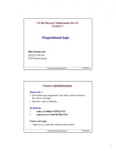
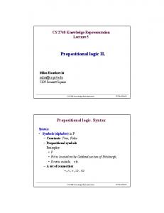
The negation operator is a unary operator that takes one operand, while the other operators are binary operators taking two operands. Definition 2.2 A formula in propositional logic is a tree defined recursively: • A formula is a leaf labeled by an atomic proposition. • A formula is a node labeled by ¬ with a single child that is a formula. • A formula is a node labeled by one of the binary operators with two children both of which are formulas. Example 2.3 Figure 2.1 shows two formulas.
2.1.2 Formulas as Strings Just as we write expressions as strings (linear sequences of symbols), we can write formulas as strings. The string associated with a formula is obtained by an inorder traversal of the tree: Algorithm 2.4 (Represent a formula by a string) Input: A formula A of propositional logic. Output: A string representation of A.
2.1 Propositional Formulas
9
Fig. 2.1 Two formulas
Call the recursive procedure Inorder(A): Inorder(F) if F is a leaf write its label return let F1 and F2 be the left and right subtrees of F Inorder(F1) write the label of the root of F Inorder(F2) If the root of F is labeled by negation, the left subtree is considered to be empty and the step Inorder(F1) is skipped. Definition 2.5 The term formula will also be used for the string with the understanding that it refers to the underlying tree. Example 2.6 Consider the left formula in Fig. 2.1. The inorder traversal gives: write the leftmost leaf labeled p, followed by its root labeled →, followed by the right leaf of the implication labeled q, followed by the root of the tree labeled ↔, and so on. The result is the string: p → q ↔ ¬ p → ¬ q. Consider now the right formula in Fig. 2.1. Performing the traversal results in the string: p → q ↔ ¬ p → ¬ q, which is precisely the same as that associated with the left formula.
10
2
Propositional Logic: Formulas, Models, Tableaux
Although the formulas are not ambiguous—the trees have entirely different structures—their representations as strings are ambiguous. Since we prefer to deal with strings, we need some way to resolve such ambiguities. There are three ways of doing this.
2.1.3 Resolving Ambiguity in the String Representation Parentheses The simplest way to avoid ambiguity is to use parentheses to maintain the structure of the tree when the string is constructed. Algorithm 2.7 (Represent a formula by a string with parentheses) Input: A formula A of propositional logic. Output: A string representation of A. Call the recursive procedure Inorder(A): Inorder(F) if F is a leaf write its label return let F1 and F2 be the left and right subtrees of F write a left parenthesis ’(’ Inorder(F1) write the label of the root of F Inorder(F2) write a right parenthesis ’)’ If the root of F is labeled by negation, the left subtree is considered to be empty and the step Inorder(F1) is skipped. The two formulas in Fig. 2.1 are now associated with two different strings and there is no ambiguity: ((p → q) ↔ ((¬ q) → (¬ p))), (p → (q ↔ (¬ (p → (¬ q))))). The problem with parentheses is that they make formulas verbose and hard to read and write.
Precedence The second way of resolving ambiguous formulas is to define precedence and associativity conventions among the operators as is done in arithmetic, so that we
2.1 Propositional Formulas
11
immediately recognize a ∗ b ∗ c + d ∗ e as (((a ∗ b) ∗ c) + (d ∗ e)). For formulas the order of precedence from high to low is as follows: ¬ ∧, ↑ ∨, ↓ → ↔, ⊕ Operators are assumed to associate to the right, that is, a ∨ b ∨ c means (a ∨ (b ∨ c)). Parentheses are used only if needed to indicate an order different from that imposed by the rules for precedence and associativity, as in arithmetic where a ∗ (b + c) needs parentheses to denote that the addition is done before the multiplication. With minimal use of parentheses, the formulas above can be written: p → q ↔ ¬ q → ¬ p, p → (q ↔ ¬ (p → ¬ q)). Additional parentheses may always be used to clarify a formula: (p ∨ q) ∧ (q ∨ r). The Boolean operators ∧, ∨, ↔, ⊕ are associative so we will often omit parentheses in formulas that have repeated occurrences of these operators: p ∨ q ∨ r ∨ s. Note that →, ↓, ↑ are not associative, so parentheses must be used to avoid confusion. Although the implication operator is assumed to be right associative, so that p → q → r unambiguously means p → (q → r), we will write the formula with parentheses to avoid confusion with (p → q) → r. Polish Notation * There will be no ambiguity if the string representing a formula is created by a preorder traversal of the tree: Algorithm 2.8 (Represent a formula by a string in Polish notation) Input: A formula A of propositional logic. Output: A string representation of A. Call the recursive procedure Preorder(A): Preorder(F) write the label of the root of F if F is a leaf return let F1 and F2 be the left and right subtrees of F Preorder(F1) Preorder(F2) If the root of F is labeled by negation, the left subtree is considered to be empty and the step Preorder(F1) is skipped.
12
2
Propositional Logic: Formulas, Models, Tableaux
Example 2.9 The strings associated with the two formulas in Fig. 2.1 are: ↔ → p q → ¬ p¬ q, →p ↔ q¬ → p¬ q and there is no longer any ambiguity. The formulas are said to be in Polish notation, named after a group of Polish logicians led by Jan Łukasiewicz. We find infix notation easier to read because it is familiar from arithmetic, so Polish notation is normally used only in the internal representation of arithmetic and logical expressions in a computer. The advantage of Polish notation is that the expression can be evaluated in the linear order that the symbols appear using a stack. If we rewrite the first formula backwards (reverse Polish notation): q¬ p¬ → qp → ↔, it can be directly compiled to the following sequence of instructions of an assembly language: Push q Negate Push p Negate Imply Push q Push p Imply Equiv The operators are applied to the top operands on the stack which are then popped and the result pushed.
2.1.4 Structural Induction Given an arithmetic expression like a ∗ b + b ∗ c, it is immediately clear that the expression is composed of two terms that are added together. In turn, each term is composed of two factors that are multiplied together. In the same way, any propositional formula can be classified by its top-level operator. Definition 2.10 Let A ∈ F . If A is not an atom, the operator labeling the root of the formula A is the principal operator of the A. Example 2.11 The principal operator of the left formula in Fig. 2.1 is ↔, while the principal operator of the right formulas is →.
2.1 Propositional Formulas
13
Structural induction is used to prove that a property holds for all formulas. This form of induction is similar to the familiar numerical induction that is used to prove that a property holds for all natural numbers (Appendix A.6). In numerical induction, the base case is to prove the property for 0 and then to prove the inductive step: assume that the property holds for arbitrary n and then show that it holds for n + 1. By Definition 2.10, a formula is either a leaf labeled by an atom or it is a tree with a principal operator and one or two subtrees. The base case of structural induction is to prove the property for a leaf and the inductive step is to prove the property for the formula obtained by applying the principal operator to the subtrees, assuming that the property holds for the subtrees. Theorem 2.12 (Structural induction) To show that a property holds for all formulas A ∈ F: 1. Prove that the property holds all atoms p. 2. Assume that the property holds for a formula A and prove that the property holds for ¬ A. 3. Assume that the property holds for formulas A1 and A2 and prove that the property holds for A1 op A2 , for each of the binary operators. Proof Let A be an arbitrary formula and suppose that (1), (2), (3) have been shown for some property. We show that the property holds for A by numerical induction on n, the height of the tree for A. For n = 0, the tree is a leaf and A is an atom p, so the property holds by (1). Let n > 0. The subtrees A are of height n − 1, so by numerical induction, the property holds for these formulas. The principal operator of A is either negation or one of the binary operators, so by (2) or (3), the property holds for A. We will later show that all the binary operators can be defined in terms negation and either disjunction or conjunction, so a proof that a property holds for all formulas can be done using structural induction with the base case and only two inductive steps.
2.1.5 Notation Unfortunately, books on mathematical logic use widely varying notation for the Boolean operators; furthermore, the operators appear in programming languages with a different notation from that used in mathematics textbooks. The following table shows some of these alternate notations.
14
2
Propositional Logic: Formulas, Models, Tableaux
Operator
Alternates
Java language
¬
∼
!
∧
&
&, &&
∨
|, ||
→
⊃, ⇒
↔
≡, ⇔
⊕
�≡
↑
|
^
2.1.6 A Formal Grammar for Formulas * This subsection assumes familiarity with formal grammars. Instead of defining formulas as trees, they can be defined as strings generated by a context-free formal grammar. Definition 2.13 Formula in propositional logic are derived from the context-free grammar whose terminals are: • An unbounded set of symbols P called atomic propositions. • The Boolean operators given in Definition 2.1. The productions of the grammar are: fml fml fml op
::= ::= ::= ::=
p for any p ∈ P ¬ fml fml op fml ∨|∧| → | ↔ | ⊕ |↑|↓
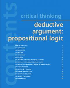
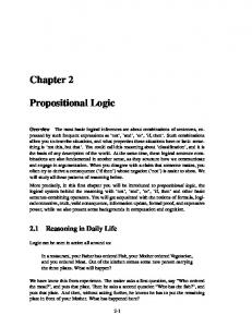
A formula is a word that can be derived from the nonterminal fml. The set of all formulas that can be derived from the grammar is denoted F . Derivations of strings (words) in a formal grammar can be represented as trees (Hopcroft et al., 2006, Sect. 4.3). The word generated by a derivation can be read off the leaves from left to right. Example 2.14 Here is a derivation of the formula p → q ↔ ¬ p → ¬ q in propositional logic; the tree representing its derivation is shown in Fig. 2.2.
2.1 Propositional Formulas
15
Fig. 2.2 Derivation tree for p → q ↔ ¬ p → ¬ q
1. 2. 3. 4. 5. 6. 7. 8. 9. 10. 11. 12. 13.
fml fml op fml fml ↔ fml fml op fml ↔ fml fml → fml ↔ fml p → fml ↔ fml p → q ↔ fml p → q ↔ fml op fml p → q ↔ fml → fml p → q ↔ ¬ fml → fml p → q ↔ ¬ p → fml p → q ↔ ¬ p → ¬ fml p → q ↔ ¬p → ¬q
The methods discussed in Sect. 2.1.2 can be used to resolve ambiguity. We can change the grammar to introduce parentheses: fml ::= (¬ fml) fml ::= (fml op fml) and then use precedence to reduce their number.
16
2
Propositional Logic: Formulas, Models, Tableaux
vI (A) = IA (A)
if A is an atom
vI (¬ A) = T vI (¬ A) = F
if vI (A) = F if vI (A) = T
vI (A1 ∨ A2 ) = F vI (A1 ∨ A2 ) = T
if vI (A1 ) = F and vI (A2 ) = F otherwise
vI (A1 ∧ A2 ) = T vI (A1 ∧ A2 ) = F
if vI (A1 ) = T and vI (A2 ) = T otherwise
vI (A1 → A2 ) = F vI (A1 → A2 ) = T
if vI (A1 ) = T and vI (A2 ) = F otherwise
vI (A1 ↑ A2 ) = F vI (A1 ↑ A2 ) = T
if vI (A1 ) = T and vI (A2 ) = T otherwise
vI (A1 ↓ A2 ) = T vI (A1 ↓ A2 ) = F
if vI (A1 ) = F and vI (A2 ) = F otherwise
vI (A1 ↔ A2 ) = T vI (A1 ↔ A2 ) = F
if vI (A1 ) = vI (A2 ) if vI (A1 ) �= vI (A2 )
vI (A1 ⊕ A2 ) = T vI (A1 ⊕ A2 ) = F
if vI (A1 ) �= vI (A2 ) if vI (A1 ) = vI (A2 )
Fig. 2.3 Truth values of formulas
2.2 Interpretations We now define the semantics—the meaning—of formulas. Consider again arithmetic expressions. Given an expression E such as a ∗ b + 2, we can assign values to a and b and then evaluate the expression. For example, if a = 2 and b = 3 then E evaluates to 8. In propositional logic, truth values are assigned to the atoms of a formula in order to evaluate the truth value of the formula.
2.2.1 The Definition of an Interpretation Definition 2.15 Let A ∈ F be a formula and let PA be the set of atoms appearing in A. An interpretation for A is a total function IA : PA �→ {T , F } that assigns one of the truth values T or F to every atom in PA . Definition 2.16 Let IA be an interpretation for A ∈ F . vIA (A), the truth value of A under IA is defined inductively on the structure of A as shown in Fig. 2.3. In Fig. 2.3, we have abbreviated vIA (A) by vI (A). The abbreviation I for IA will be used whenever the formula is clear from the context. Example 2.17 Let A = (p → q) ↔ (¬ q → ¬ p) and let IA be the interpretation: IA (p) = F,
IA (q) = T .
2.2 Interpretations
17
The truth value of A can be evaluated inductively using Fig. 2.3: vI (p) vI (q) vI (p → q) vI (¬ q) vI (¬ p) vI (¬ q → ¬ p) vI ((p → q) ↔ (¬ q → ¬ p))
= = = = = = =
IA (p) = F IA (q) = T T F T T T.
Partial Interpretations * We will later need the following definition, but you can skip it for now: Definition 2.18 Let A ∈ F . A partial interpretation for A is a partial function IA : PA �→ {T , F } that assigns one of the truth values T or F to some of the atoms in PA . It is possible that the truth value of a formula can be determined in a partial interpretation. Example 2.19 Consider the formula A = p ∧ q and the partial interpretation that assigns F to p. Clearly, the truth value of A is F . If the partial interpretation assigned T to p, we cannot compute the truth value of A.
2.2.2 Truth Tables A truth table is a convenient format for displaying the semantics of a formula by showing its truth value for every possible interpretation of the formula. Definition 2.20 Let A ∈ F and supposed that there are n atoms in PA . A truth table is a table with n + 1 columns and 2n rows. There is a column for each atom in PA , plus a column for the formula A. The first n columns specify the interpretation I that maps atoms in PA to {T , F }. The last column shows vI (A), the truth value of A for the interpretation I . Since each of the n atoms can be assigned T or F independently, there are 2n interpretations and thus 2n rows in a truth table.
18
2
Propositional Logic: Formulas, Models, Tableaux
Example 2.21 Here is the truth table for the formula p → q: p T T F F
p→q T F T T
q T F T F
When the formula A is complex, it is easier to build a truth table by adding columns that show the truth value for subformulas of A. Example 2.22 Here is a truth table for the formula (p → q) ↔ (¬ q → ¬ p) from Example 2.17: p T T F F
q T F T F
p→q T F T T
¬p F F T T
¬q F T F T
¬q → ¬p T F T T
(p → q) ↔ (¬ q → ¬ p) T T T T
A convenient way of computing the truth value of a formula for a specific interpretation I is to write the value T or F of I (pi ) under each atom pi and then to write down the truth values incrementally under each operator as you perform the computation. Each step of the computation consists of choosing an innermost subformula and evaluating it. Example 2.23 The computation of the truth value of (p → q) ↔ (¬ q → ¬ p) for the interpretation I (p) = T and I (q) = F is: (p T T T T T T
→
F F
q) F F F F F F
↔
(¬
T
T T T T T
q F F F F F F
→
¬
F F F
F F F F
p) T T T T T T
2.2 Interpretations
19
If the computations for all subformulas are written on the same line, the truth table from Example 2.22 can be written as follows: p T T F F
q T F T F
(p T T F F
→ T F T T
q) T F T F
↔ T T T T
(¬ F T F T
q T F T F
→ T F T T
¬ F F T T
p) T T F F
2.2.3 Understanding the Boolean Operators The natural reading of the Boolean operators ¬ and ∧ correspond with their formal semantics as defined in Fig. 2.3. The operators ↑ and ↓ are simply negations of ∧ and ∨. Here we comment on the operators ∨, ⊕ and →, whose formal semantics can be the source of confusion.
Inclusive or vs. Exclusive or Disjunction ∨ is inclusive or and is a distinct operator from ⊕ which is exclusive or. Consider the compound statement: At eight o’clock ‘I will go to the movies’ or ‘I will go to the theater’.
The intended meaning is ‘movies’ ⊕ ‘theater’, because I can’t be in both places at the same time. This contrasts with the disjunctive operator ∨ which evaluates to true when either or both of the statements are true: Do you want ‘popcorn’ or ‘candy’?
This can be denoted by ‘popcorn’ ∨ ‘candy’, because it is possible to want both of them at the same time. For ∨, it is sufficient for one statement to be true for the compound statement to be true. Thus, the following strange statement is true because the truth of the first statement by itself is sufficient to ensure the truth of the compound statement: ‘Earth is farther from the sun than Venus’ ∨ ‘1 + 1 = 3’.
The difference between ∨ and ⊕ is seen when both subformulas are true: ‘Earth is farther from the sun than Venus’ ∨ ‘1 + 1 = 2’. ‘Earth is farther from the sun than Venus’ ⊕ ‘1 + 1 = 2’.
The first statement is true but the second is false.
20
2
Propositional Logic: Formulas, Models, Tableaux
Inclusive or vs. Exclusive or in Programming Languages When or is used in the context of programming languages, the intention is usually inclusive or: if (index < min || index > max) /* There is an error */ The truth of one of the two subexpressions causes the following statements to be executed. The operator || is not really a Boolean operator because it uses shortcircuit evaluation: if the first subexpression is true, the second subexpression is not evaluated, because its truth value cannot change the decision to execute the following statements. There is an operator | that performs true Boolean evaluation; it is usually used when the operands are bit vectors: mask1 = 0xA0; mask2 = 0x0A; mask = mask1 | mask2; Exclusive or ^ is used to implement encoding and decoding in error-correction and cryptography. The reason is that when used twice, the original value can be recovered. Suppose that we encode bit of data with a secret key: codedMessage = data ^ key; The recipient of the message can decode it by computing: clearMessage = codedMessage ^ key; as shown by the following computation: clearMessage == == == == ==
codedMessage ^ key (data ^ key) ^ key data ^ (key ^ key) data ^ false data
Implication The operator of p →q is called material implication; p is the antecedent and q is the consequent. Material implication does not claim causation; that is, it does not assert there the antecedent causes the consequent (or is even related to the consequent in any way). A material implication merely states that if the antecedent is true the consequent must be true (see Fig. 2.3), so it can be falsified only if the antecedent is true and the consequent is false. Consider the following two compound statements: ‘Earth is farther from the sun than Venus’ → ‘1 + 1 = 3’.
is false since the antecedent is true and the consequent is false, but:
2.3 Logical Equivalence
21
‘Earth is farther from the sun than Mars’ → ‘1 + 1 = 3’.
is true! The falsity of the antecedent by itself is sufficient to ensure the truth of the implication.
2.2.4 An Interpretation for a Set of Formulas � Definition 2.24 Let S = {A1 , . . .} be a set of formulas and let PS = i PAi , that is, PS is the set of all the atoms that appear in the formulas of S. An interpretation for S is a function IS : PS �→ {T , F }. For any Ai ∈ S, vIS (Ai ), the truth value of Ai under IS , is defined as in Definition 2.16. The definition of PS as the union of the sets of atoms in the formulas of S ensures that each atom is assigned exactly one truth value. Example 2.25 Let S = {p → q, p, q ∧ r, p ∨ s ↔ s ∧ q} and let IS be the interpretation: IS (p) = T ,
IS (q) = F,
IS (r) = T ,
IS (s) = T .
The truth values of the elements of S can be evaluated as: vI (p → q) vI (p) vI (q ∧ r) vI (p ∨ s) vI (s ∧ q) vI (p ∨ s ↔ s ∧ q)
= = = = = =
F IS (p) = T F T F F.
2.3 Logical Equivalence Definition 2.26 Let A1 , A2 ∈ F . If vI (A1 ) = vI (A2 ) for all interpretations I , then A1 is logically equivalent to A2 , denoted A1 ≡ A2 . Example 2.27 Is the formula p ∨ q logically equivalent to q ∨ p? There are four distinct interpretations that assign to the atoms p and q: I (p)
I (q)
vI (p ∨ q)
vI (q ∨ p)
T T F F
T F T F
T T T F
T T T F
22
2
Propositional Logic: Formulas, Models, Tableaux
Since p ∨ q and q ∨ p agree on all the interpretations, p ∨ q ≡ q ∨ p. This example can be generalized to arbitrary formulas: Theorem 2.28 Let A1 , A2 ∈ F . Then A1 ∨ A2 ≡ A2 ∨ A1 . Proof Let I be an arbitrary interpretation for A1 ∨ A2 . Obviously, I is also an interpretation for A2 ∨ A1 since PA1 ∪ PA2 = PA2 ∪ PA1 . Since PA1 ⊆ PA1 ∪ PA2 , I assigns truth values to all atoms in A1 and can be considered to be an interpretation for A1 . Similarly, I can be considered to be an interpretation for A2 . Now vI (A1 ∨ A2 ) = T if and only if either vI (A1 ) = T or vI (A2 ) = T , and vI (A2 ∨ A1 ) = T if and only if either vI (A2 ) = T or vI (A1 ) = T . If vI (A1 ) = T , then: vI (A1 ∨ A2 ) = T = vI (A2 ∨ A1 ), and similarly if vI (A2 ) = T . Since I was arbitrary, A1 ∨ A2 ≡ A2 ∨ A1 . This type of argument will be used frequently. In order to prove that something is true of all interpretations, we let I be an arbitrary interpretation and then write a proof without using any property that distinguishes one interpretation from another.
2.3.1 The Relationship Between ↔ and ≡ Equivalence, ↔, is a Boolean operator in propositional logic and can appear in formulas of the logic. Logical equivalence, ≡, is not a Boolean operator; instead, is a notation for a property of pairs of formulas in propositional logic. There is potential for confusion because we are using a similar vocabulary both for the object language, in this case the language of propositional logic, and for the metalanguage that we use reason about the object language. Equivalence and logical equivalence are, nevertheless, closely related as shown by the following theorem: Theorem 2.29 A1 ≡ A2 if and only if A1 ↔ A2 is true in every interpretation. Proof Suppose that A1 ≡ A2 and let I be an arbitrary interpretation; then vI (A1 ) = vI (A2 ) by definition of logical equivalence. From Fig. 2.3, vI (A1 ↔ A2 ) = T . Since I was arbitrary, vI (A1 ↔ A2 ) = T in all interpretations. The proof of the converse is similar.
2.3 Logical Equivalence
23
Fig. 2.4 Subformulas
2.3.2 Substitution Logical equivalence justifies substitution of one formula for another. Definition 2.30 A is a subformula of B if A is a subtree of B. If A is not the same as B, it is a proper subformula of B. Example 2.31 Figure 2.4 shows a formula (the left formula from Fig. 2.1) and its proper subformulas. Represented as strings, (p → q) ↔ (¬ p → ¬ q) contains the proper subformulas: p → q, ¬ p → ¬ q, ¬ p, ¬ q, p, q. Definition 2.32 Let A be a subformula of B and let A� be any formula. B{A ← A� }, the substitution of A� for A in B, is the formula obtained by replacing all occurrences of the subtree for A in B by A� . Example 2.33 Let B = (p → q) ↔ (¬ p → ¬ q), A = p → q and A� = ¬ p ∨ q. B{A ← A� } = (¬ p ∨ q) ↔ (¬ q → ¬ p).
Given a formula A, substitution of a logically equivalent formula for a subformula of A does not change its truth value under any interpretation. Theorem 2.34 Let A be a subformula of B and let A� be a formula such that A ≡ A� . Then B ≡ B{A ← A� }.
24
2
Propositional Logic: Formulas, Models, Tableaux
Proof Let I be an arbitrary interpretation. Then vI (A) = vI (A� ) and we must show that vI (B) = vI (B � ). The proof is by induction on the depth d of the highest occurrence of the subtree A in B. If d = 0, there is only one occurrence of A, namely B itself. Obviously, vI (B) = vI (A) = vI (A� ) = vI (B � ). If d �= 0, then B is ¬ B1 or B1 op B2 for some formulas B1 , B2 and operator op. In B1 , the depth of A is less than d. By the inductive hypothesis, vI (B1 ) = vI (B1� ) = vI (B1 {A ← A� }), and similarly vI (B2 ) = vI (B2� ) = vI (B2 {A ← A� }). By the definition of v on the Boolean operators, vI (B) = vI (B � ).
2.3.3 Logically Equivalent Formulas Substitution of logically equivalence formulas is frequently done, for example, to simplify a formula, and it is essential to become familiar with the common equivalences that are listed in this subsection. Their proofs are elementary from the definitions and are left as exercises.
Absorption of Constants Let us extend the syntax of Boolean formulas to include the two constant atomic propositions true and false. (Another notation is � for true and ⊥ for false.) Their semantics are defined by I (true) = T and I (false) = F for any interpretation. Do not confuse these symbols in the object language of propositional logic with the truth values T and F used to define interpretations. Alternatively, it is possible to regard true and false as abbreviations for the formulas p ∨ ¬ p and p ∧ ¬ p, respectively. The appearance of a constant in a formula can collapse the formula so that the binary operator is no longer needed; it can even make a formula become a constant whose truth value no longer depends on the non-constant subformula. A ∨ true A ∨ false A → true A → false A ↔ true A ↔ false
≡ ≡ ≡ ≡ ≡ ≡
true A true ¬A A ¬A
A ∧ true A ∧ false true → A false → A A ⊕ true A ⊕ false
≡ ≡ ≡ ≡ ≡ ≡
A false A true ¬A A
2.3 Logical Equivalence
25
Identical Operands Collapsing can also occur when both operands of an operator are the same or one is the negation of another. A A A ∨ ¬A A→A A↔A ¬A
≡ ≡ ≡ ≡ ≡ ≡
¬¬A A∧A true true true A ↑ A¬ A
≡ ≡
A A ∧ ¬A A⊕A ≡
A∨A false
≡ false A↓A
Commutativity, Associativity and Distributivity The binary Boolean operators are commutative, except for implication. A∨B ≡ B ∨A A↔B ≡ B ↔A A↑B ≡ B ↑A
A∧B ≡ B ∧A A⊕B ≡ B ⊕A A↓B ≡ B ↓A
If negations are added, the direction of an implication can be reversed: A → B ≡ ¬B → ¬A The formula ¬ B → ¬ A is the contrapositive of A → B. Disjunction, conjunction, equivalence and non-equivalence are associative. A ∨ (B ∨ C) ≡ (A ∨ B) ∨ C A ↔ (B ↔ C) ≡ (A ↔ B) ↔ C
A ∧ (B ∧ C) ≡ (A ∧ B) ∧ C A ⊕ (B ⊕ C) ≡ (A ⊕ B) ⊕ C
Implication, nor and nand are not associative. Disjunction and conjunction distribute over each other. A ∨ (B ∧ C) ≡ (A ∨ B) ∧ (A ∨ C) A ∧ (B ∨ C) ≡ (A ∧ B) ∨ (A ∧ C)
Defining One Operator in Terms of Another When proving theorems about propositional logic using structural induction, we have to prove the inductive step for each of the binary operators. It will simplify proofs if we can eliminate some of the operators by replacing subformulas with formulas that use another operator. For example, equivalence can be eliminated be-
26
2
Propositional Logic: Formulas, Models, Tableaux
cause it can be defined in terms of conjunction and implication. Another reason for eliminating operators is that many algorithms on propositional formulas require that the formulas be in a normal form, using a specified subset of the Boolean operators. Here is a list of logical equivalences that can be used to eliminate operators. A↔B A→B A∨B A∨B
≡ ≡ ≡ ≡
(A → B) ∧ (B → A) ¬A ∨ B ¬ (¬ A ∧ ¬ B) ¬A → B
A⊕B A→B A∧B A∧B
≡ ≡ ≡ ≡
¬ (A → B) ∨ ¬ (B → A) ¬ (A ∧ ¬ B) ¬ (¬ A ∨ ¬ B) ¬ (A → ¬ B)
The definition of conjunction in terms of disjunction and negation, and the definition of disjunction in terms of conjunction and negation are called De Morgan’s laws.
2.4 Sets of Boolean Operators * From our earliest days in school, we are taught that there are four basic operators in arithmetic: addition, subtraction, multiplication and division. Later on, we learn about additional operators like modulo and absolute value. On the other hand, multiplication and division are theoretically redundant because they can be defined in terms of addition and subtraction. In this section, we will look at two issues: What Boolean operators are there? What sets of operators are adequate, meaning that all other operators can be defined using just the operators in the set?
2.4.1 Unary and Binary Boolean Operators Since there are only two Boolean values T and F , the number of possible n-place n operators is 22 , because for each of the n arguments we can choose either of the two values T and F and for each of these 2n n-tuples of arguments we can choose the value of the operator to be either T or F . We will restrict ourselves to one- and two-place operators. 1 The following table shows the 22 = 4 possible one-place operators, where the first column gives the value of the operand x and the other columns give the value of the nth operator ◦n (x): x
◦1
◦2
◦3
◦4
T F
T T
T F
F T
F F
2.4 Sets of Boolean Operators *
27
x1
x2
◦1
◦2
◦3
◦4
◦5
◦6
◦7
◦8
T T F F
T F T F
T T T T
T T T F
T T F T
T T F F
T F T T
T F T F
T F F T
T F F F
x1
x2
◦9
◦10
◦11
◦12
◦13
◦14
◦15
◦16
T T F F
T F T F
F T T T
F T T F
F T F T
F T F F
F F T T
F F T F
F F F T
F F F F
Fig. 2.5 Two-place Boolean operators
Of the four one-place operators, three are trivial: ◦1 and ◦4 are the constant operators, and ◦2 is the identity operator which simply maps the operand to itself. The only non-trivial one-place operator is ◦3 which is negation. 2 There are 22 = 16 two-place operators (Fig. 2.5). Several of the operators are trivial: ◦1 and ◦16 are constant; ◦4 and ◦6 are projection operators, that is, their value is determined by the value of only one of operands; ◦11 and ◦13 are the negations of the projection operators. The correspondence between the operators in the table and those we defined in Definition 2.1 are shown in the following table, where the operators in the right-hand column are the negations of those in the left-hand column. op
name
◦2 ◦8 ◦5 ◦7
disjunction conjunction implication equivalence
symbol
op
name
symbol
∨ ∧ → ↔
◦15 ◦9
nor nand
↓ ↑
◦10
exclusive or
⊕
The operator ◦12 is the negation of implication and is not used. Reverse implication, ◦3 , is used in logic programming (Chap. 11); its negation, ◦14 , is not used.
2.4.2 Adequate Sets of Operators Definition 2.35 A binary operator ◦ is defined from a set of operators {◦1 , . . . , ◦n } iff there is a logical equivalence A1 ◦A2 ≡ A, where A is a formula constructed from occurrences of A1 and A2 using the operators {◦1 , . . . , ◦n }. The unary operator ¬
28
2
Propositional Logic: Formulas, Models, Tableaux
is defined by a formula ¬ A1 ≡ A, where A is constructed from occurrences of A1 and the operators in the set. Theorem 2.36 The Boolean operators ∨, ∧, →, ↔, ⊕, ↑, ↓ can be defined from negation and one of ∨, ∧, →. Proof The theorem follows by using the logical equivalences in Sect. 2.3.3. The nand and nor operators are the negations of conjunction and disjunction, respectively. Equivalence can be defined from implication and conjunction and nonequivalence can be defined using these operators and negation. Therefore, we need only →, ∨, ∧, but each of these operators can be defined by one of the others and negation as shown by the equivalences on page 26. It may come as a surprise that it is possible to define all Boolean operators from either nand or nor alone. The equivalence ¬ A ≡ A ↑ A is used to define negation from nand and the following sequence of equivalences shows how conjunction can be defined: (A ↑ B) ↑ (A ↑ B) ¬ ((A ↑ B) ∧ (A ↑ B)) ¬ (A ↑ B) ¬ ¬ (A ∧ B) A ∧ B.
≡ ≡ ≡ ≡
by the definition of ↑ by idempotence by the definition of ↑ by double negation
From the formulas for negation and conjunction, all other operators can be defined. Similarly definitions are possible using nor. In fact it can be proved that only nand and nor have this property. Theorem 2.37 Let ◦ be a binary operator that can define negation and all other binary operators by itself. Then ◦ is either nand or nor. Proof We give an outline of the proof and leave the details as an exercise. Suppose that ◦ is an operator that can define all the other operators. Negation must be defined by an equivalence of the form: ¬ A ≡ A ◦ · · · ◦ A. Any binary operator op must be defined by an equivalence: A1 op A2 ≡ B1 ◦ · · · ◦ Bn , where each Bi is either A1 or A2 . (If ◦ is not associative, add parentheses as necessary.) We will show that these requirements impose restrictions on ◦ so that it must be nand or nor. Let I be any interpretation such that vI (A) = T ; then F = vI (¬ A) = vI (A ◦ · · · ◦ A).
2.5 Satisfiability, Validity and Consequence
29
Prove by induction on the number of occurrences of ◦ that vI (A1 ◦ A2 ) = F when vI (A1 ) = T and vI (A2 ) = T . Similarly, if I is an interpretation such that vI (A) = F , prove that vI (A1 ◦ A2 ) = T . Thus the only freedom we have in defining ◦ is in the case where the two operands are assigned different truth values: A1
A2
A1 ◦ A2
T T F F
T F T F
F T or F T or F T
If ◦ is defined to give the same truth value T for these two lines then ◦ is nand, and if ◦ is defined to give the same truth value F then ◦ is nor. The remaining possibility is that ◦ is defined to give different truth values for these two lines. Prove by induction that only projection and negated projection are definable in the sense that: B1 ◦ · · · ◦ Bn ≡ ¬ · · · ¬ Bi for some i and zero or more negations.
2.5 Satisfiability, Validity and Consequence We now define the fundamental concepts of the semantics of formulas: Definition 2.38 Let A ∈ F . • A is satisfiable iff vI (A) = T for some interpretation I . A satisfying interpretation is a model for A. • A is valid, denoted |= A, iff vI (A) = T for all interpretations I . A valid propositional formula is also called a tautology. • A is unsatisfiable iff it is not satisfiable, that is, if vI (A) = F for all interpretations I . • A is falsifiable, denoted �|= A, iff it is not valid, that is, if vI (A) = F for some interpretation v. These concepts are illustrated in Fig. 2.6. The four semantical concepts are closely related. Theorem 2.39 Let A ∈ F . A is valid if and only if ¬ A is unsatisfiable. A is satisfiable if and only if ¬ A is falsifiable.
30
2
Propositional Logic: Formulas, Models, Tableaux
Fig. 2.6 Satisfiability and validity of formulas
Proof Let I be an arbitrary interpretation. vI (A) = T if and only if vI (¬ A) = F by the definition of the truth value of a negation. Since I was arbitrary, A is true in all interpretations if and only if ¬ A is false in all interpretations, that is, iff ¬ A is unsatisfiable. If A is satisfiable then for some interpretation I , vI (A) = T . By definition of the truth value of a negation, vI (¬ A) = F so that ¬ A is falsifiable. Conversely, if vI (¬ A) = F then vI (A) = T .
2.5.1 Decision Procedures in Propositional Logic Definition 2.40 Let U ⊆ F be a set of formulas. An algorithm is a decision procedure for U if given an arbitrary formula A ∈ F , it terminates and returns the answer yes if A ∈ U and the answer no if A �∈ U . If U is the set of satisfiable formulas, a decision procedure for U is called a decision procedure for satisfiability, and similarly for validity. By Theorem 2.39, a decision procedure for satisfiability can be used as a decision procedure for validity. To decide if A is valid, apply the decision procedure for satisfiability to ¬ A. If it reports that ¬ A is satisfiable, then A is not valid; if it reports that ¬ A is not satisfiable, then A is valid. Such an decision procedure is called a refutation procedure, because we prove the validity of a formula by refuting its negation. Refutation procedures can be efficient algorithms for deciding validity, because instead of checking that the formula is always true, we need only search for a falsifying counterexample. The existence of a decision procedure for satisfiability in propositional logic is trivial, because we can build a truth table for any formula. The truth table in Example 2.21 shows that p → q is satisfiable, but not valid; Example 2.22 shows that (p → q) ↔ (¬ q → ¬ p) is valid. The following example shows an unsatisfiable formula.
2.5 Satisfiability, Validity and Consequence
31
Example 2.41 The formula (p ∨ q) ∧ ¬ p ∧ ¬ q is unsatisfiable because all lines of its truth table evaluate to F . p T T F F
q T F T F
p∨q T T T F
¬p F F T T
¬q F T F T
(p ∨ q) ∧ ¬ p ∧ ¬ q F F F F
The method of truth tables is a very inefficient decision procedure because we need to evaluate a formula for each of 2n possible interpretations, where n is the number of distinct atoms in the formula. In later chapters we will discuss more efficient decision procedures for satisfiability, though it is extremely unlikely that there is a decision procedure that is efficient for all formulas (see Sect. 6.7).
2.5.2 Satisfiability of a Set of Formulas The concept of satisfiability can be extended to a set of formulas. Definition 2.42 A set of formulas U = {A1 , . . .} is (simultaneously) satisfiable iff there exists an interpretation I such that vI (Ai ) = T for all i. The satisfying interpretation is a model of U . U is unsatisfiable iff for every interpretation I , there exists an i such that vI (Ai ) = F . Example 2.43 The set U1 = {p, ¬ p ∨ q, q ∧ r} is simultaneously satisfiable by the interpretation which assigns T to each atom, while the set U2 = {p, ¬ p ∨ q, ¬ p} is unsatisfiable. Each formula in U2 is satisfiable by itself, but the set is not simultaneously satisfiable. The proofs of the following elementary theorems are left as exercises. Theorem 2.44 If U is satisfiable, then so is U − {Ai } for all i. Theorem 2.45 If U is satisfiable and B is valid, then U ∪ {B} is satisfiable. Theorem 2.46 If U is unsatisfiable, then for any formula B, U ∪ {B} is unsatisfiable. Theorem 2.47 If U is unsatisfiable and for some i, Ai is valid, then U − {Ai } is unsatisfiable.
32
2
Propositional Logic: Formulas, Models, Tableaux
2.5.3 Logical Consequence Definition 2.48 Let U be a set of formulas and A a formula. A is a logical consequence of U , denoted U |= A, iff every model of U is a model of A. The formula A need not be true in every possible interpretation, only in those interpretations which satisfy U , that is, those interpretations which satisfy every formula in U . If U is empty, logical consequence is the same as validity. Example 2.49 Let A = (p ∨ r) ∧ (¬ q ∨ ¬ r). Then A is a logical consequence of {p, ¬ q}, denoted {p, ¬ q} |= A, since A is true in all interpretations I such that I (p) = T and I (q) = F . However, A is not valid, since it is not true in the interpretation I � where I � (p) = F , I � (q) = T , I � (r) = T . The caveat concerning ↔ and ≡ also applies to → and |=. Implication, →, is an operator in the object language, while |= is a symbol for a concept in the metalanguage. However, as with equivalence, the two concepts are related: Theorem 2.50 U |= A if and only if |=
� i
Ai → A.
� � Definition 2.51 i=n i=1 Ai is an abbreviation for A1 ∧ · · · ∧ An . The notation i is used if the bounds � are obvious from the context or if the set of formulas is infinite. A similar notation is used for disjunction. Example 2.52 From Example 2.49, {p, ¬ q} |= (p ∨ r) ∧ (¬ q ∨ ¬ r), so by Theorem 2.50, |= (p ∧ ¬ q) → (p ∨ r) ∧ (¬ q ∨ ¬ r). The proof of Theorem 2.50, as well as the proofs of the following two theorems are left as exercises. Theorem 2.53 If U |= A then U ∪ {B} |= A for any formula B. Theorem 2.54 If U |= A and B is valid then U − {B} |= A.
2.5.4 Theories * Logical consequence is the central concept in the foundations of mathematics. Valid logical formulas such as p ∨ q ↔ q ∨ p are of little mathematical interest. It is much more interesting to assume that a set of formulas is true and then to investigate the consequences of these assumptions. For example, Euclid assumed five formulas about geometry and deduced an extensive set of logical consequences. The formal definition of a mathematical theory is as follows. Definition 2.55 Let T be a set of formulas. T is closed under logical consequence iff for all formulas A, if T |= A then A ∈ T . A set of formulas that is closed under logical consequence is a theory. The elements of T are theorems.
2.6 Semantic Tableaux
33
Theories are constructed by selecting a set of formulas called axioms and deducing their logical consequences. Definition 2.56 Let T be a theory. T is said to be axiomatizable iff there exists a set of formulas U such that T = {A | U |= A}. The set of formulas U are the axioms of T . If U is finite, T is said to be finitely axiomatizable. Arithmetic is axiomatizable: There is a set of axioms developed by Peano whose logical consequences are theorems of arithmetic. Arithmetic is not finitely axiomatizable, because the induction axiom is not by a single axiom but an axiom scheme with an instance for each property in arithmetic.
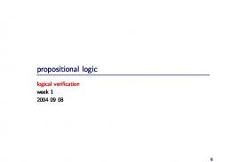
2.6 Semantic Tableaux The method of semantic tableaux is an efficient decision procedure for satisfiability (and by duality validity) in propositional logic. We will use semantic tableaux extensively in the next chapter to prove important theorems about deductive systems. The principle behind semantic tableaux is very simple: search for a model (satisfying interpretation) by decomposing the formula into sets of atoms and negations of atoms. It is easy to check if there is an interpretation for each set: a set of atoms and negations of atoms is satisfiable iff the set does not contain an atom p and its negation ¬ p. The formula is satisfiable iff one of these sets is satisfiable. We begin with some definitions and then analyze the satisfiability of two formulas to motivate the construction of semantic tableaux.
2.6.1 Decomposing Formulas into Sets of Literals Definition 2.57 A literal is an atom or the negation of an atom. An atom is a positive literal and the negation of an atom is a negative literal. For any atom p, {p, ¬ p} is a complementary pair of literals. For any formula A, {A, ¬ A} is a complementary pair of formulas. A is the complement of ¬ A and ¬ A is the complement of A. Example 2.58 In the set of literals {¬ p, q, r, ¬ r}, q and r are positive literals, while ¬ p and ¬ r are negative literals. The set contains the complementary pair of literals {r, ¬ r}. Example 2.59 Let us analyze the satisfiability of the formula: A = p ∧ (¬ q ∨ ¬ p) in an arbitrary interpretation I , using the inductive rules for the evaluation of the truth value of a formula.
34
2
Propositional Logic: Formulas, Models, Tableaux
• The principal operator of A is conjunction, so vI (A) = T if and only if both vI (p) = T and vI (¬ q ∨ ¬ p) = T . • The principal operator of ¬ q ∨ ¬ p is disjunction, so vI (¬ q ∨ ¬ p) = T if and only if either vI (¬ q) = T or vI (¬ p) = T . • Integrating the information we have obtained from this analysis, we conclude that vI (A) = T if and only if either: 1. 2.
vI (p) = T and vI (¬ q) = T , or vI (p) = T and vI (¬ p) = T .
A is satisfiable if and only if there is an interpretation such that (1) holds or an interpretation such that (2) holds. We have reduced the question of the satisfiability of A to a question about the satisfiability of sets of literals. Theorem 2.60 A set of literals is satisfiable if and only if it does not contain a complementary pair of literals. Proof Let L be a set of literals that does not contain a complementary pair. Define the interpretation I by: I (p) = T I (p) = F
if p ∈ L, if ¬ p ∈ L.
The interpretation is well-defined—there is only one value assigned to each atom in L—since there is no complementary pair of literals in L. Each literal in L evaluates to T so L is satisfiable. Conversely, if {p, ¬ p} ⊆ L, then for any interpretation I for the atoms in L, either vI (p) = F or vI (¬ p) = F , so L is not satisfiable. Example 2.61 Continuing the analysis of the formula A = p ∧ (¬ q ∨ ¬ p) from Example 2.59, A is satisfiable if and only at least one of the sets {p, ¬ p} and {p, ¬ q} does not contain a complementary pair of literals. Clearly, only the second set does not contain a complementary pair of literals. Using the method described in Theorem 2.60, we obtain the interpretation: I (p) = T ,
I (q) = F.
We leave it to the reader to check that for this interpretation, vI (A) = T . The following example shows what happens if a formula is unsatisfiable. Example 2.62 Consider the formula: B = (p ∨ q) ∧ (¬ p ∧ ¬ q).
2.6 Semantic Tableaux
35
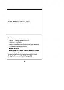
Fig. 2.7 Semantic tableaux
The analysis of the formula proceeds as follows: • vI (B) = T if and only if vI (p ∨ q) = T and vI (¬ p ∧ ¬ q) = T . • Decomposing the conjunction, vI (B)=T if and only if vI (p ∨ q) = T and vI (¬ p) = vI (¬ q) = T . • Decomposing the disjunction, vI (B) = T if and only if either: 1. vI (p) = vI (¬ p) = vI (¬ q) = T , or 2. vI (q) = vI (¬ p) = vI (¬ q) = T . Both sets of literals {p, ¬ p, ¬ q} and {q, ¬ p, ¬ q} contain complementary pairs, so by Theorem 2.60, both set of literals are unsatisfiable. We conclude that it is impossible to find a model for B; in other words, B is unsatisfiable.
2.6.2 Construction of Semantic Tableaux The decomposition of a formula into sets of literals is rather difficult to follow when expressed textually, as we did in Examples 2.59 and 2.62. In the method of semantic tableaux, sets of formulas label nodes of a tree, where each path in the tree represents the formulas that must be satisfied in one possible interpretation. The initial formula labels the root of the tree; each node has one or two child nodes depending on how a formula labeling the node is decomposed. The leaves are labeled by the sets of literals. A leaf labeled by a set of literals containing a complementary pair of literals is marked ×, while a leaf labeled by a set not containing a complementary pair is marked �. Figure 2.7 shows semantic tableaux for the formulas from the examples. The tableau construction is not unique; here is another tableau for B: (p ∨ q) ∧ (¬ p ∧ ¬ q) ↓ p ∨ q, ¬ p ∧ ¬ q � � p, ¬ p ∧ ¬ q q, ¬ p ∧ ¬ q ↓ ↓ p, ¬ p, ¬ q q, ¬ p, ¬ q × ×
36
2
Propositional Logic: Formulas, Models, Tableaux
α
α1
α2
β
β1
β2
¬ ¬ A1 A1 ∧ A2 ¬ (A1 ∨ A2 ) ¬ (A1 → A2 ) ¬ (A1 ↑ A2 ) A1 ↓ A2 A1 ↔ A2 ¬ (A1 ⊕ A2 )
A1 A1 ¬ A1 A1 A1 ¬ A1 A1 →A2 A1 →A2
A2 ¬ A2 ¬ A2 A2 ¬ A2 A2 →A1 A2 →A1
¬ (B1 ∧ B2 ) B1 ∨ B2 B1 → B2 B1 ↑ B2 ¬ (B1 ↓ B2 ) ¬ (B1 ↔ B2 ) B1 ⊕ B2
¬ B1 B1 ¬ B1 ¬ B1 B1 ¬ (B1 →B2 ) ¬ (B1 →B2 )
¬ B2 B2 B2 ¬ B2 B2 ¬ (B2 →B1 ) ¬ (B2 →B1 )
Fig. 2.8 Classification of α- and β-formulas
It is constructed by branching to search for a satisfying interpretation for p ∨ q before searching for one for ¬ p ∧ ¬ q. The first tableau contains fewer nodes, showing that it is preferable to decompose conjunctions before disjunctions. A concise presentation of the rules for creating a semantic tableau can be given if formulas are classified according to their principal operator (Fig. 2.8). If the formula is a negation, the classification takes into account both the negation and the principal operator. α-formulas are conjunctive and are satisfiable only if both subformulas α1 and α2 are satisfied, while β-formulas are disjunctive and are satisfied even if only one of the subformulas β1 or β2 is satisfiable. Example 2.63 The formula p ∧ q is classified as an α-formula because it is true if and only if both p and q are true. The formula ¬ (p ∧ q) is classified as a β-formula. It is logically equivalent to ¬ p ∨ ¬ q and is true if and only if either ¬ p is true or ¬ q is true. We now give the algorithm for the construction of a semantic tableau for a formula in propositional logic. Algorithm 2.64 (Construction of a semantic tableau) Input: A formula φ of propositional logic. Output: A semantic tableau T for φ all of whose leaves are marked. Initially, T is a tree consisting of a single root node labeled with the singleton set {φ}. This node is not marked. Repeat the following step as long as possible: Choose an unmarked leaf l labeled with a set of formulas U (l) and apply one of the following rules. • U (l) is a set of literals. Mark the leaf closed × if it contains a complementary pair of literals. If not, mark the leaf open �. • U (l) is not a set of literals. Choose a formula in U (l) which is not a literal. Classify the formula as an α-formula A or as a β-formula B and perform one of the following steps according to the classification:
2.6 Semantic Tableaux
37
– A is an α-formula. Create a new node l � as a child of l and label l � with: U (l � ) = (U (l) − {A}) ∪ {A1 , A2 }. (In the case that A is ¬ ¬ A1 , there is no A2 .) – B is a β-formula. Create two new nodes l � and l �� as children of l. Label l � with: U (l � ) = (U (l) − {B}) ∪ {B1 }, and label l �� with: U (l �� ) = (U (l) − {B}) ∪ {B2 }.
Definition 2.65 A tableau whose construction has terminated is a completed tableau. A completed tableau is closed if all its leaves are marked closed. Otherwise (if some leaf is marked open), it is open.
2.6.3 Termination of the Tableau Construction Since each step of the algorithm decomposes one formula into one or two simpler formulas, it is clear that the construction of the tableau for any formula terminates, but it is worth proving this claim. Theorem 2.66 The construction of a tableau for any formula φ terminates. When the construction terminates, all the leaves are marked × or �. Proof Let us assume that ↔ and ⊕ do not occur in the formula φ; the extension of the proof for these cases is left as an exercise. Consider an unmarked leaf l that is chosen to be expanded during the construction of the tableau. Let b(l) be the total number of binary operators in all formulas in U (l) and let n(l) be the total number of negations in U (l). Define: W (l) = 3 · b(l) + n(l). For example, if U (l) = {p ∨ q, ¬ p ∧ ¬ q}, then W (l) = 3 · 2 + 2 = 8. Each step of the algorithm adds either a new node l � or a pair of new nodes � l , l �� as children of l. We claim that W (l � ) < W (l) and, if there is a second node, W (l �� ) < W (l). Suppose that A = ¬ (A1 ∨ A2 ) and that the rule for this α-formula is applied at l to obtain a new leaf l � labeled: U (l � ) = (U (l) − {¬ (A1 ∨ A2 )}) ∪ {¬ A1 , ¬ A2 }. Then: W (l � ) = W (l) − (3 · 1 + 1) + 2 = W (l) − 2 < W (l),
38
2
Propositional Logic: Formulas, Models, Tableaux
because one binary operator and one negation are removed, while two negations are added. Suppose now that B = B1 ∨ B2 and that the rule for this β-formula is applied at l to obtain two new leaves l � , l �� labeled: U (l � ) = (U (l) − {B1 ∨ B2 }) ∪ {B1 }, U (l �� ) = (U (l) − {B1 ∨ B2 }) ∪ {B2 }. Then: W (l � ) ≤ W (l) − (3 · 1) < W (l),
W (l �� ) ≤ W (l) − (3 · 1) < W (l).
We leave it to the reader to prove that W (l) decreases for the other α- and βformulas. The value of W (l) decreases as each branch in the tableau is extended. Since, obviously, W (l) ≥ 0, no branch can be extended indefinitely and the construction of the tableau must eventually terminate. A branch can always be extended if its leaf is labeled with a set of formulas that is not a set of literals. Therefore, when the construction of the tableau terminates, all leaves are labeled with sets of literals and each is marked open or closed by the first rule of the algorithm.
2.6.4 Improving the Efficiency of the Algorithm * The algorithm for constructing a tableau is not deterministic: at most steps, there is a choice of which leaf to extend and if the leaf contains more than one formula which is not a literal, there is a choice of which formula to decompose. This opens the possibility of applying heuristics in order to cause the tableau to be completed quickly. We saw in Sect. 2.6.2 that it is better to decompose α-formulas before βformulas to avoid duplication. Tableaux can be shortened by closing a branch if it contains a formula and its negation and not just a pair of complementary literals. Clearly, there is no reason to continue expanding a node containing: (p ∧ (q ∨ r)),
¬ (p ∧ (q ∨ r)).
We leave it as an exercise to prove that this modification preserves the correctness of the algorithm. There is a lot of redundancy in copying formulas from one node to another: U (l � ) = (U (l) − {A}) ∪ {A1 , A2 }. In a variant of semantic tableaux called analytic tableaux (Smullyan, 1968), when a new node is created, it is labeled only with the new formulas:
2.7 Soundness and Completeness
39
U (l � ) = {A1 , A2 }. The algorithm is changed so that the formula to be decomposed is selected from the set of formulas labeling the nodes on the branch from the root to a leaf (provided, of course, that the formula has not already been selected). A leaf is marked closed if two complementary literals (or formulas) appear in the labels of one or two nodes on a branch, and a leaf is marked open if is not closed but there are no more formulas to decompose. Here is an analytic tableau for the formula B from Example 2.62, where the formula p ∨ q is not copied from the second node to the third when p ∧ q is decomposed: (p ∨ q) ∧ (¬ p ∧ ¬ q) ↓ p ∨ q, ¬ p ∧ ¬ q ↓ ¬ p, ¬ q � � p q × × We prefer to use semantic tableaux because it is easy to see which formulas are candidates for decomposition and how to mark leaves.
2.7 Soundness and Completeness The construction of a semantic tableau is a purely formal. The decomposition of a formula depends solely on its syntactical properties: its principal operator and—if it is a negation—the principal operator of the formula that is negated. We gave several examples to motivate semantic tableau, but we have not yet proven that the algorithm is correct. We have not connected the syntactical outcome of the algorithm (Is the tableau closed or not?) with the semantical concept of truth value. In this section, we prove that the algorithm is correct in the sense that it reports that a formula is satisfiable or unsatisfiable if and only if there exists or does not exist a model for the formula. The proof techniques of this section should be studied carefully because they will be used again and again in other logical systems. Theorem 2.67 Soundness and completeness Let T be a completed tableau for a formula A. A is unsatisfiable if and only if T is closed. Here are some corollaries that follow from the theorem. Corollary 2.68 A is satisfiable if and only if T is open. Proof A is satisfiable iff (by definition) A is not unsatisfiable iff (by Theorem 2.67) T is not closed iff (by definition) T is open.
40
2
Propositional Logic: Formulas, Models, Tableaux
Corollary 2.69 A is valid if and only if the tableau for ¬ A closes. Proof A is valid iff ¬ A is unsatisfiable iff the tableau for ¬ A closes. Corollary 2.70 The method of semantic tableaux is a decision procedure for validity in propositional logic. Proof Let A be a formula of propositional logic. By Theorem 2.66, the construction of the semantic tableau for ¬ A terminates in a completed tableau. By the previous corollary, A is valid if and only if the completed tableau is closed. The forward direction of Corollary 2.69 is called completeness: if A is valid, we can discover this fact by constructing a tableau for ¬ A and the tableau will close. The converse direction is called soundness: any formula A that the tableau construction claims valid (because the tableau for ¬ A closes) actually is valid. Invariably in logic, soundness is easier to show than completeness. The reason is that while we only include in a formal system rules that are obviously sound, it is hard to be sure that we haven’t forgotten some rule that may be needed for completeness. At the extreme, the following vacuous algorithm is sound but far from complete! Algorithm 2.71 (Incomplete decision procedure for validity) Input: A formula A of propositional logic. Output: A is not valid. Example 2.72 If the rule for ¬ (A1 ∨ A2 ) is omitted, the construction of the tableau is still sound, but it is not complete, because it is impossible to construct a closed tableau for the obviously valid formula A = ¬ p ∨ p. Label the root of the tableau with the negation ¬ A = ¬ (¬ p ∨ p); there is now no rule that can be used to decompose the formula.
2.7.1 Proof of Soundness The theorem to be proved is: if the tableau T for a formula A closes, then A is unsatisfiable. We will prove a more general theorem: if Tn , the subtree rooted at node n of T , closes then the set of formulas U (n) labeling n is unsatisfiable. Soundness is the special case for the root. To make the proof easier to follow, we will use A1 ∧ A2 and B1 ∨ B2 as representatives of the classes of α- and β-formulas, respectively. Proof of Soundness The proof is by induction on the height hn of the node n in Tn . Clearly, a closed leaf is labeled by an unsatisfiable set of formulas. Recall (Definition 2.42) that a set of formulas is unsatisfiable iff for any interpretation the truth value of at least one formula is false. In the inductive step, if the children of a node n
2.7 Soundness and Completeness
41
are labeled by an unsatisfiable set of formulas, then: (a) either the unsatisfiable formula also appears in the label of n, or (b) the unsatisfiable formulas in the labels of the children were used to construct an unsatisfiable formula in the label of n. Let us write out the formal proof. For the base case, hn = 0, assume that Tn closes. Since hn = 0 means that n is a leaf, U (n) must contain a complementary set of literals so it is unsatisfiable. For the inductive step, let n be a node such that hn > 0 in Tn . We need to show that Tn is closed implies that U (n) is unsatisfiable. By the inductive hypothesis, we can assume that for any node m of height hm < hn , if Tm closes, then U (m) is unsatisfiable. Since hn > 0, the rule for some α- or β-formula was used to create the children of n: n : {A1 ∧ A2 } ∪ U0 n : {B1 ∨ B2 } ∪ U0 @ @
n� : {A1 , A2 } ∪ U0
n� : {B1 } ∪ U0
@ @
@ n�� : {B2 } ∪ U0
Case 1: U (n) = {A1 ∧ A2 } ∪ U0 and U (n� ) = {A1 , A2 } ∪ U0 for some (possibly empty) set of formulas U0 . Clearly, Tn� is also a closed tableau and since hn� = hn − 1, by the inductive hypothesis U (n� ) is unsatisfiable. Let I be an arbitrary interpretation. There are two possibilities: • vI (A0 ) = F for some formula A0 ∈ U0 . But U0 ⊂ U (n) so U (n) is also unsatisfiable. • Otherwise, vI (A0 ) = T for all A0 ∈ U0 , so vI (A1 ) = F or vI (A2 ) = F . Suppose that vI (A1 ) = F . By the definition of the semantics of ∧, this implies that vI (A1 ∧ A2 ) = F . Since A1 ∧ A2 ∈ U (n), U (n) is unsatisfiable. A similar argument holds if vI (A2 ) = F . Case 2: U (n) = {B1 ∨ B2 } ∪ U0 , U (n� ) = {B1 } ∪ U0 , and U (n�� ) = {B2 } ∪ U0 for some (possibly empty) set of formulas U0 . Clearly, Tn� and Tn�� are also closed tableaux and since hn� ≤ hn − 1 and hn�� ≤ hn − 1, by the inductive hypothesis U (n� ) and U (n�� ) are both unsatisfiable. Let I be an arbitrary interpretation. There are two possibilities: • vI (B0 ) = F for some formula B0 ∈ U0 . But U0 ⊂ U (n) so U (n) is also unsatisfiable. • Otherwise, vI (B0 ) = T for all B0 ∈ U0 , so vI (B1 ) = F (since U (n� ) is unsatisfiable) and vI (B2 ) = F (since U (n�� ) is unsatisfiable). By the definition of the semantics of ∨, this implies that vI (B1 ∨ B2 ) = F . Since B1 ∨ B2 ∈ U (n), U (n) is unsatisfiable.
42
2
Propositional Logic: Formulas, Models, Tableaux
2.7.2 Proof of Completeness The theorem to be proved is: if A is unsatisfiable then every tableau for A closes. Completeness is much more difficult to prove than soundness. For soundness, we had a single (though arbitrary) closed tableau for a formula A and we proved that A is unsatisfiable by induction on the structure of a tableau. Here we need to prove that no matter how the tableau for A is constructed, it must close. Rather than prove that every tableau must close, we prove the contrapositive (Corollary 2.68): if some tableau for A is open (has an open branch), then A is satisfiable. Clearly, there is a model for the set of literals labeling the leaf of an open branch. We extend this to an interpretation for A and then prove by induction on the length of the branch that the interpretation is a model of the sets of formulas labeling the nodes on the branch, including the singleton set {A} that labels the root. Let us look at some examples. Example 2.73 Let A = p ∧ (¬ q ∨ ¬ p). We have already constructed the tableau for A which is reproduced here: p ∧ (¬ q ∨ ¬ p) ↓ p, ¬ q ∨ ¬ p � � p, ¬ q p, ¬ p � × The interpretation I (p) = T , I (q) = F defined by assigning T to the literals labeling the leaf of the open branch is clearly a model for A. Example 2.74 Now let A = p ∨ (q ∧ ¬ q); here is a tableau for A: p ∨ (q ∧ ¬ q) � � p q ∧ ¬q � ↓ q, ¬ q × The open branch of the tableau terminates in a leaf labeled with the singleton set of literals {p}. We can conclude that any model for A must define I (p) = T . However, an interpretation for A must also define an assignment to q and the leaf gives us no guidance as to which value to choose for I (q). But it is obvious that it doesn’t matter what value is assigned to q; in either case, the interpretation will be a model of A. To prove completeness we need to show that the assignment of T to the literals labeling the leaf of an open branch can be extended to a model of the formula labeling the root. There are four steps in the proof:
2.7 Soundness and Completeness
43
1. Define a property of sets of formulas; 2. Show that the union of the formulas labeling nodes in an open branch has this property; 3. Prove that any set having this property is satisfiable; 4. Note that the formula labeling the root is in the set. Definition 2.75 Let U be a set of formulas. U is a Hintikka set iff: 1. For all atoms p appearing in a formula of U , either p �∈ U or ¬ p �∈ U . 2. If A ∈ U is an α-formula, then A1 ∈ U and A2 ∈ U . 3. If B ∈ U is a β-formula, then B1 ∈ U or B2 ∈ U . Example 2.76 U , the union of the set of formulas labeling the nodes in the open branch of Example 2.74, is {p, p ∨ (q ∧ ¬ q)}. We claim that U is a Hintikka set. Condition (1) obviously holds since there is only one literal p in U and ¬ p �∈ U . Condition (2) is vacuous. For Condition (3), B = p ∨ (q ∧ ¬ q) ∈ U is a β-formula and B1 = p ∈ U . Condition (1) requires that a Hintikka set not contain a complementary pair of literals, which to be expected on an open branch of a tableau. Conditions (2) and (3) ensure that U is downward saturated, that is, U contains sufficient subformulas so that the decomposition of the formula to be satisfied will not take us out of U . In turn, this ensures that an interpretation defined by the set of literals in U will make all formulas in U true. The second step of the proof of completeness is to show that the set of formulas labeling the nodes in an open branch is a Hintikka set. � Theorem 2.77 Let l be an open leaf in a completed tableau T . Let U = i U (i), where i runs over the set of nodes on the branch from the root to l. Then U is a Hintikka set. Proof In the construction of the semantic tableau, there are no rules for decomposing a literal p or ¬ p. Thus if a literal p or ¬ p appears for the first time in U (n) for some n, the literal will be copied into U (k) for all nodes k on the branch from n to l, in particular, p ∈ U (l) or ¬ p ∈ U (l). This means that all literals in U appear in U (l). Since the branch is open, no complementary pair of literals appears in U (l), so Condition (1) holds for U . Suppose that A ∈ U is an α-formula. Since the tableau is completed, A was the formula selected for decomposing at some node n in the branch from the root to l. Then {A1 , A2 } ⊆ U (n� ) ⊆ U , so Condition (2) holds. Suppose that B ∈ U is an β-formula. Since the tableau is completed, B was the formula selected for decomposing at some node n in the branch from the root to l. Then either B1 ∈ U (n� ) ⊆ U or B2 ∈ U (n� ) ⊆ U , so Condition (3) holds.
44
2
Propositional Logic: Formulas, Models, Tableaux
The third step of the proof is to show that a Hintikka set is satisfiable. Theorem 2.78 (Hintikka’s Lemma) Let U be a Hintikka set. Then U is satisfiable. Proof We define an interpretation and then show that the interpretation is a model of U . Let PU be set of all atoms appearing in all formulas of U . Define an interpretation I : PU �→ {T , F } as follows: I (p) = T I (p) = F I (p) = T
if p ∈ U, if ¬ p ∈ U, if p �∈ U and ¬ p �∈ U.
Since U is a Hintikka set, by Condition (1) I is well-defined, that is, every atom in PU is given exactly one value. Example 2.74 demonstrates the third case: the atom q appears in a formula of U so q ∈ PU , but neither the literal q nor its complement ¬ q appear in U . The atom is arbitrarily mapped to the truth value T . We show by structural induction that for any A ∈ U, vI (A) = T . • If A is an atom p, then vI (A) = vI (p) = I (p) = T since p ∈ U . • If A is a negated atom ¬ p, then since ¬ p ∈ U , I (p) = F , so vI (A) = vI (¬ p) = T . • If A is an α-formula, by Condition (2) A1 ∈ U and A2 ∈ U . By the inductive hypothesis, vI (A1 ) = vI (A2 ) = T , so vI (A) = T by definition of the conjunctive operators. • If A is β-formula B, by Condition (3) B1 ∈ U or B2 ∈ U . By the inductive hypothesis, either vI (B1 ) = T or vI (B2 ) = T , so vI (A) = vI (B) = T by definition of the disjunctive operators. Proof of Completeness Let T be a completed open tableau for A. Then U , the union of the labels of the nodes on an open branch, is a Hintikka set by Theorem 2.77. Theorem 2.78 shows an interpretation I can be found such that U is simultaneously satisfiable in I . A, the formula labeling the root, is an element of U so I is a model of A.
2.8 Summary The presentation of propositional logic was carried out in a manner that we will use for all systems of logic. First, the syntax of formulas is given. The formulas are defined as trees, which avoids ambiguity and simplifies the description of structural induction. The second step is to define the semantics of formulas. An interpretation is a mapping of atomic propositions to the values {T , F }. An interpretation is used to give a truth value to any formula by induction on the structure of the formula, starting from atoms and proceeding to more complex formulas using the definitions of the Boolean operators.
2.9 Further Reading
45
A formula is satisfiable iff it is true in some interpretation and it is valid iff is true in all interpretations. Two formulas whose values are the same in all interpretations are logically equivalent and can be substituted for each other. This can be used to show that for any formula, there exists a logically equivalent formula that uses only negation and either conjunction or disjunction. While truth tables can be used as a decision procedure for the satisfiability or validity of formulas of propositional logic, semantic tableaux are usually much more efficient. In a semantic tableau, a tree is constructed during a search for a model of a formula; the construction is based upon the structure of the formula. A semantic tableau is closed if the formula is unsatisfiable and open if it is satisfiable. We proved that the algorithm for semantic tableaux is sound and complete as a decision procedure for satisfiability. This theorem connects the syntactical aspect of a formula that guides the construction of the tableau with its meaning. The central concept in the proof is that of a Hintikka set, which gives conditions that ensure that a model can be found for a set of formulas.
2.9 Further Reading The presentation of semantic tableaux follows that of Smullyan (1968) although he uses analytic tableaux. Advanced textbooks that also use tableaux are Nerode and Shore (1997) and Fitting (1996).
2.10 Exercises 2.1 Draw formation trees and construct truth tables for (p → (q → r)) → ((p → q) → (p → r)), (p → q) → p, ((p → q) → p) → p. 2.2 Prove that there is a unique formation tree for every derivation tree. 2.3 Prove the following logical equivalences: A ∧ (B ∨ C) ≡ (A ∧ B) ∨ (A ∧ C), A ∨ B ≡ ¬ (¬ A ∧ ¬ B), A ∧ B ≡ ¬ (¬ A ∨ ¬ B), A → B ≡ ¬ A ∨ B, A → B ≡ ¬ (A ∧ ¬ B). 2.4 Prove ((A ⊕ B) ⊕ B) ≡ A and ((A ↔ B) ↔ B) ≡ A.
46
2
Propositional Logic: Formulas, Models, Tableaux
2.5 Simplify A ∧ (A ∨ B) and A ∨ (A ∧ B). 2.6 Prove the following logical equivalences using truth tables, semantic tableaux or Venn diagrams: A→B A→B A∧B A↔B
≡ ≡ ≡ ≡
A ↔ (A ∧ B), B ↔ (A ∨ B), (A ↔ B) ↔ (A ∨ B), (A ∨ B) → (A ∧ B).
2.7 Prove |= (A → B) ∨ (B → C). 2.8 Prove or disprove: |= ((A → B) → B) → B, |= (A ↔ B) ↔ (A ↔ (B ↔ A)). 2.9 Prove: |= ((A ∧ B) → C) → ((A → C) ∨ (B → C)). This formula may seem strange since it could be misinterpreted as saying that if C follows from A ∧ B, then it follows from one or the other of A or B. To clarify this, show that: {A ∧ B → C} |= (A → C) ∨ (B → C), but: {A ∧ B → C} �|= A → C, {A ∧ B → C} �|= B → C. 2.10 Complete the proof that ↑ and ↓ can each define all unary and binary Boolean operators (Theorem 2.37). 2.11 Prove that ∧ and ∨ cannot define all Boolean operators. 2.12 Prove that {¬ , ↔} cannot define all Boolean operators. 2.13 Prove that ↑ and ↓ are not associative. 2.14 Prove that if U is satisfiable then U ∪ {B} is not necessarily satisfiable. 2.15 Prove Theorems 2.44–2.47 on the satisfiability of sets of formulas. 2.16 Prove Theorems 2.50–2.54 on logical consequence.
References
47
2.17 Prove that for a set of axioms U , T (U ) is closed under logical consequence (see Definition 2.55). 2.18 Complete the proof that the construction of a semantic tableau terminates (Theorem 2.66). 2.19 Prove that the method of semantic tableaux remains sound and complete if a tableau can be closed non-atomically. 2.20 Manna (1974) Let ifte be a tertiary (3-place) operator defined by: A
B
C
ifte(A, B, C)
T T T T F F F F
T T F F T T F F
T F T F T F T F
T T F F T F T F
The operator can be defined using infix notation as: if A then B else C. 1. Prove that if then else by itself forms an adequate sets of operators if the use of the constant formulas true and false is allowed. 2. Prove: |= if A then B else C ≡ (A → B) ∧ (¬ A → C). 3. Add a rule for the operator if then else to the algorithm for semantic tableaux.
References M. Fitting. First-Order Logic and Automated Theorem Proving (Second Edition). Springer, 1996. J.E. Hopcroft, R. Motwani, and J.D. Ullman. Introduction to Automata Theory, Languages and Computation (Third Edition). Addison-Wesley, 2006. Z. Manna. Mathematical Theory of Computation. McGraw-Hill, New York, NY, 1974. Reprinted by Dover, 2003. A. Nerode and R.A. Shore. Logic for Applications (Second Edition). Springer, 1997. R.M. Smullyan. First-Order Logic. Springer-Verlag, 1968. Reprinted by Dover, 1995.
http://www.springer.com/978-1-4471-4128-0