Propositional Reasoning that Tracks Probabilistic Reasoning Hanti Lin∗
Kevin T. Kelly† ‡
Carnegie Mellon University March 19, 2012
Abstract This paper concerns the extent to which uncertain propositional reasoning can track probabilistic reasoning, and addresses kinematic problems that extend the familiar Lottery paradox. An acceptance rule assigns to each Bayesian credal state p a propositional belief revision method Bp , which specifies an initial belief state Bp (⊤), that is revised to the new propositional belief state B(E) upon receipt of information E. An acceptance rule tracks Bayesian conditioning when Bp (E) = Bp|E (⊤), for every E such that p(E) > 0; namely, when acceptance by propositional belief revision equals Bayesian conditioning followed by acceptance. Standard proposals for uncertain acceptance and belief revision do not track Bayesian conditioning. The “Lockean” rule that accepts propositions above a probability threshold is subject to the familiar lottery paradox (Kyburg 1961), and we show that it is also subject to new and more stubborn paradoxes when the tracking property is taken into account. Moreover, we show that the familiar AGM approach to belief revision (Harper 1975 and Alchourrón, Gärdenfors, and Makinson 1985) cannot be realized in a sensible way by any uncertain acceptance rule that tracks Bayesian conditioning. Finally, we present a plausible, alternative approach that tracks Bayesian conditioning and avoids all of the paradoxes. It combines an odds-based acceptance rule proposed originally by Levi (1996) with a non-AGM belief revision method proposed originally by Shoham (1987). ∗
e-mail:
[email protected] e-mail:
[email protected] ‡ This work was supported generously by the National Science Foundation under grant 0750681 and the John Templeton Foundation under grant 24145. Any opinions, findings, and conclusions or recommendations expressed in this material are those of the authors and do not necessarily reflect the views of the National Science Foundation or the John Templeton Foundation. †
1
1
An Old Riddle of Uncertain Acceptance
There are two widespread practices for modeling the doxastic state of a subject— as a probability measure over propositions or as a single proposition corresponding to the conjunction of all propositions the subject believes. One straightforward way to relate propositional belief to probabilistic belief is to accept only propositions of probability one. However, that skeptical approach severely restricts the scope and practical relevance of propositional reasoning, so it is natural to seek a more liberal standard for acceptance. One natural idea, called the Lockean rule in honor of John Locke, who proposed something like it, is to accept all and only the logical consequences of the set of all sufficiently probable propositions, whose probabilities are no less than some fixed threshold t strictly less than one. Alas, however the threshold for acceptance is set, the Lockean rule leads to acceptance of inconsistency, a difficulty known as the lottery paradox (Kyburg 1961). Suppose that the threshold is 2/3. Now consider a fair lottery with 3 tickets. Then the degree of belief that a given ticket loses is 2/3, so it is accepted that each ticket loses. That entails that no ticket wins. With probability one some ticket wins, so that proposition is also accepted. The conjunction of the accepted propositions is contradictory. In general, if t is the threshold, a lottery with more than 1/(1 − t) tickets suffices for acceptance of inconsistency.
2
Two New Riddles of Uncertain Acceptance
The lottery paradox concerns static consistency. But there is also the kinematic question of how to revise one’s propositional belief state in light of new evidence or suppositions. Probabilistic reasoning has its own, familiar revision method, namely, Bayesian conditioning. Mismatches between propositional belief revision and Bayesian conditioning are another potential source of conundrums for uncertain acceptance. Unlike the lottery paradox, these riddles cannot be avoided by the expedient of raising the probabilistic standard for acceptance to a sufficiently high level short of full belief. For the first riddle, suppose that there are three tickets and consider the Lockean acceptance rule with threshold 3/4, at which the lottery paradox is easily avoided. Suppose further that the lottery is not fair: ticket 1 wins with probability 1/2 and tickets 2 and 3 win with probability 1/4. Then it is just above the threshold that ticket 2 loses and that ticket 3 loses, which entails that ticket 1 wins. Now entertain the new information that ticket 3 has been removed from the lottery, so it cannot win. Since ruling out a competing ticket seems only to provide further evidence that ticket 1 will win, it is strange to then retract one’s belief that ticket 1 wins. But the Lockean rule does just that. By Bayesian conditioning, the probability that ticket 3 wins is reset to
2
0 and the odds between tickets 1 and 2 remain 2:1, so the probability that ticket 1 wins is 2/3. Therefore, it is no longer accepted that ticket 1 wins, since that proposition is neither sufficiently probable by itself nor entailed by a set of sufficiently probable propositions, where sufficient probability means probability no less than 3/4. It is important to recognize that the first riddle is geometrical rather than logical (figure 1). Let H1 be the proposition that ticket 1 wins, and similarly for H2 , H3 . The
p
H1
H3
p H3
H2
H2
T H1
H3 h3
Figure 1: the first riddle space of all probability distributions over the three tickets consists of a triangle in the Euclidean plane whose corners have coordinates (1, 0, 0), (0, 1, 0), and (0, 0, 1), which are the extremal distributions that concentrate all probability on a single ticket. The assumed distribution p over tickets then corresponds to the point p = (1/2, 1/4, 1/4) in the triangle. The conditional distribution p|¬H3 = p(·|¬H3 ) is the point (2/3, 1/3, 0), which lies on a ray through p that originates from corner 3, holding the odds H1 : H2 constant. Each zone in the triangle is labeled with the strongest proposition accepted at the probability measures inside. The acceptance zone for H1 is a parallel-sided diamond that results from the intersection of the above-threshold zones for ¬H2 and ¬H3 , since it is assumed that the accepted propositions are closed under conjunction. The rule leaves the inner triangle as the acceptance zone for the tautology ⊤. The riddle can now be seen to result from the simple, geometrical fact that p lies near the bottom corner of the diamond, which is so acute that conditioning carries p outside of the diamond. If the bottom corner of the diamond is made more blunt, to match the slope of the conditioning ray, then the paradox does not arise. The riddle can be summarized by saying that the Lockean rule fails to satisfy the following, diachronic principle for acceptance: accepted beliefs are not to be retracted when their logical consequences are learned. Assuming that accepted propositions are closed under entailment, let Bp denote the strongest proposition accepted in probabilistic credal state p. So H is accepted at p if and only if Bp |= H. Then the principle may
3
be stated succinctly as follows, where p|E denotes the conditional distribution p(·|E): Bp |= H and H |= E =⇒ Bp|E |= H.
(1)
Philosophers of science speak of hypothetico-deductivism as the view that observing a logical consequence of a theory provides evidence in favor of the theory. Since it would be strange to retract a theory in light of new, positive evidence, we refer to the proposed principle as Hypothetico-deductive Monotonicity. One Lockean response to the preceding riddle is to adopt a higher acceptance threshold for disjunctions than for conjunctions (figure 2) so that the acceptance zone for H1 is closed under conditioning on ¬H3 . But now a different and, in a sense, complemenp
H3
H1 p H2
H3
T H2
H3
H1
h3 = p H3
Figure 2: second riddle tary riddle emerges. For suppose that the credal state is p, just inside the zone for accepting that either ticket 1 or 2 will win and close to, but outside of the zone for accepting that ticket 1 will win. The Lockean rule accepts that ticket 2 loses no matter whether one learns that ticket 3 wins (i.e. p moves to p|H3 ) or that ticket 3 loses (i.e. p moves to p|¬H3 ), but the lockean rule refuses to accept that ticket 2 loses until one actually learns what happens with ticket 3. That violates the following principle:1 Bp|E |= H and Bp|¬E |= H =⇒ Bp |= H,
(2)
which we call Case Reasoning. 1
The principle is analogous in spirit to the reflection principle (van Fraassen 1984), which, in this context, might be expressed by saying that if you know that you will accept a proposition regardless what you learn, you should accept it already. Also, a non-conglomerable probability measure has the feature that some B is less probable than it is conditional on each Hi . Schervish, Seidenfeld, and Kadane (1984) show that every finitely additive measure is non-conglomerable in some partition. In that case, any sensible acceptance rule would fail to satisfy reasoning by cases. Some experts advocate finitely additive probabilities and others view non-conglomerability as a paradoxical feature. For us, acceptance is relative to a partition (question), a topic we discuss in detail in Lin and Kelly (2011), so non-conglomerability does not necessarily arise in the given partition.
4
The two new riddles add up to one big riddle: there is, in fact, no ad hoc manipulation of distinct thresholds for distinct propositions that avoids both riddles.2 The first riddle picks up where the second riddle leaves off and there are thresholds that generate both riddles at once. Unlike the lottery paradox, which requires more tickets as the Lockean threshold is raised, one of the two new riddles obtains for every possible combination of thresholds, as long as there are at least three tickets and the thresholds have values less than one. So although it may be tempting to address the lottery paradox by raising the thresholds in response to the number of tickets, even that possibility is ruled out by the new riddles. All of the Lockean rules have the wrong shape.
3
The Propositional Space of Reasons
Part of what is jarring about the riddles is that they undermine one of the most plausible motives for considering acceptance at all: reasoning directly with propositions, without having to constantly consult the underlying probabilities. In the first riddle, observed logical consequences H result in rejection of H. In the second riddle, propositional reasoning by cases fails so that, for example, one could not rely on logic to justify policy (e.g., the policy achieves the desired objective in any case). Although one accepts propositions, the riddles witness that one has not really entered into a purely propositional “space of reasons” (Sellars 1956). The accepted propositions are mere, epiphenomenal shadows cast by the underlying probabilities, which evolve according to their own, more fundamental rules. Full entry into a propositional space of reasons demands a tighter relationship between acceptance and probabilistic conditioning. The riddles would be resolved by an improved acceptance rule that allows one to enter the propositional system, kick away the underlying probabilities, and still end up exactly where a Bayesian conditionalizer would end up—i.e., by an acceptance rule that realizes a perfect, pre-established harmony between propositional and probabilistic reasoning. The realization of such a perfect harmony, without peeking at the underlying probabilities, is far more challenging than merely to avoid acceptance of mutually inconsistent propositions. Perfect harmony will be shown to be impossible to achieve if one insists on employing the popular AGM approach to propositional belief revision. Then, we exhibit a collection of rules that do achieve perfect harmony with Bayesian conditioning.
4
Questions, Answers, and Credal States
Let Q = {Hi : i ∈ I} be a countable collection of mutually exclusive and exhaustive propositions representing a question to which H1 , . . . , Hi , . . . are the (complete) an2
The claim is a special case of theorem 3 in Lin and Kelly (2011).
5
swers. Let A denote the least σ-algebra containing Q (i.e., the set of all disjunctions of complete answers together with the unsatisfiable proposition ⊥). Let P denote the set of all countably additive probability measures on A, which will be referred to as credal states. In the three-ticket lottery, for example, Q = {H1 , H2 , H3 }, Hi says that ticket i wins, and P is the triangle (simplex) of probability distributions over the three answers.
5
Belief Revision
A belief state is just a deductively closed set of propositions; but for the sake of convenience we identity each belief state with the conjunction of all propositions believed. A belief revision method is a mapping B : A → A, understood as specifying the initial belief state B(⊤), which would evolve into new belief state B(E) upon revision on information E.3 Hypothetico-deductive Monotonicity, for example, can now be stated in terms of belief revision, rather than in terms of Bayesian conditioning:4 B(⊤) |= H and H |= E =⇒ B(E) |= H.
(3)
Case Reasoning has a similar statement:5 B(E) |= H and B(¬E) |= H =⇒ B(⊤) |= H.
6
(4)
When Belief Revision Tracks Bayesian Conditioning
A credal state represents not only one’s degrees of belief but also how they should be updated according to the Bayesian ideal. So the qualitative counterpart of a credal state should be an initial belief state plus a qualitative strategy for revising it. Accordingly, define an acceptance rule to be a function B that assigns to each credal state p a belief revision method Bp . Then Bp (⊤) is the belief state accepted unconditionally at credal state p, and proposition H is accepted (unconditionally) by rule B at credal state p if and only if Bp (⊤) |= X.6 3 Readers more familiar with the belief revision operator notation ∗ (Alchourrón, Gärdenfors, and Makinson 1985) may employ the translation rule: B(⊤) ∗ E = B(E). Note that B(⊤) is understood as the initial belief state rather than revision on the tautology. 4 Hypothetico-deductive Monotonicity is strictly weaker than the principle called Cautious Monotonicity in the nonmonotonic logic literature: B(X) |= Y and B(X) |= Z =⇒ B(X ∧ Z) |= Y . 5 Case Reasoning is an instance of the principle called Or in the nonmonotonic logic literature: B(X) |= Z and B(Y ) |= Z =⇒ B(X ∨ Y ) |= Z. 6 The following, conditional acceptance Ramsey tests translate our framework into notation familiar in the logic of epistemic conditionals:
p E⇒H
⇐⇒
Bp (E) |= H;
(5)
E |∼ p H
⇐⇒
Bp (E) |= H.
(6)
6
Each revision allows for a choice between two possible courses of action, starting at credal state p. According to the first course of action, the subject accepts propositional belief state Bp (⊤) and then revises it propositionally to obtain the new propositional belief state Bp (E) (i.e., the left-lower path in figure 3). According to the second course Bayesian conditioning
p
p
E
acceptance
acceptance
Bp(E) = Bp E(T)
Bp(T) belief revision
Figure 3: Belief revision tracks Bayesian conditioning of action, she first conditions p to obtain the posterior credal state p|E and then accepts Bp|E (⊤) (i.e., the upper-right path in figure 3). Pre-established harmony requires that the two processes should always agree (i.e., the diagram should always commute). Accordingly, say that acceptance rule B tracks conditioning if and only if: Bp (E) = Bp|E (⊤),
(7)
for each credal state p and proposition E in A such that p(E) > 0. In short, acceptance followed by belief revision equals Bayesian conditioning followed by acceptance.
7
Accretive Belief Revision
It is easy to achieve perfect tracking: just define Bp (E) according to equation (7). To avoid triviality, one must specify what would count as a propositional approach to belief revision that does not essentially peek at probabilities to decide what to do. An obvious and popular idea is simply to conjoin new information with one’s old beliefs to obtain new beliefs, as long as no contradiction results. This idea is usually separated We are indebted to Hannes Leitgeb (2010) for the idea of framing our discussion in terms of conditional acceptance, which he presented at the Opening Celebration of the Center for Formal Epistemology at Carnegie Mellon University. Our own approach (Lin and Kelly 2011), prior to seeing his work, was to formulate the issues in terms of conditional logic, via a probabilistic Ramsey test, which involves more cumbersome notation and an irrelevant commitment to an epistemic interpretation of conditionals.
7
into two parts: belief revision method B satisfies Inclusion if and only if:7 B(⊤) ∧ E |= B(E).
(8)
Method B satisfies Preservation if and only if: B(⊤) is consistent with E =⇒ B(E) |= B(⊤) ∧ E.
(9)
These axioms are widely understood to be the least controversial axioms in the muchdiscussed AGM theory of belief revision, due to Harper (1975) and Alchourrón, Gärdenfors, and Makinson (1985). A belief revision method is accretive if and only if it satisfies both Inclusion and Preservation. An acceptance rule is accretive if and only if each belief revision method Bp it assigns is accretive.
8
Sensible, Tracking Acceptance Cannot Be Accretive
Accretion sounds plausible enough when beliefs are certain, but it is not very intuitive when beliefs are accepted at probabilities less than 1. For example, suppose that we have two friends—Nogot and Havit—and we know for sure that at most one owns a Ford. The question is: who owns a Ford? There are three potential answers: “Nogot” vs. “Havit” vs. “nobody” (figure 4). Now, Nogot shows us car keys and his driver’s nobody
p
Nogot
p somebody Nogot
Havit
Figure 4: How Preservation may fail plausibly license and Havit does nothing, so we think that it is pretty probable that Nogot has a Ford (i.e., credal state p is close to the acceptance zone for “Nogot”). Suppose, further, that “Havit” is a bit more probable than “nobody” (i.e., credal state p is a bit closer to the “Havit” corner than to the “nobody” corner). So the strongest proposition we 7
Inclusion is equivalent to Case Reasoning, assuming the axiom called Success: B(E) |= E.
8
accept is the disjunction of “Nogot” with “Havit”, namely “somebody”. Unfortunately, Nogot was only pretending to own a Ford. Suppose that now we learn the negation of “Nogot”. What would we accept then? Note that the new information “¬Nogot” undermines the main reason (i.e., “Nogot”) for accepting “somebody”, in spite of the fact that the new information is still compatible with the old belief state. So it seems plausible to drop the old belief “somebody” in the new belief state, i.e., to violate the Preservation axiom. That intuition agrees with Bayesian conditioning: the posterior credal state p|¬Nogot is almost half way between the two unrefuted answers, so it is plausible for the new belief state to be neutral between the two unrefuted answers. If it is further stipulated that Havit actually owns a Ford, then we obtain Lehrer’s (1965) no-false-lemma variant of Gettier’s (1963) celebrated counterexample to justified true belief as an analysis of knowledge. At credal state p, we have justified, true, disjunctive belief that someone owns a Ford, which falls short of knowledge because the disjunctive belief’s reason relies so essentially on a false disjunct that, if the false disjunct were become doubtful, the disjunctive belief would be retracted. Any theory of rational belief that models this paradigmatic situation must violate the Preservation axiom. The preceding intuitions are vindicated by the following no-go theorem. First, we define some properties that a sensible acceptance rule should have. To begin with, we exclude skeptical acceptance rules that accept complete answers to Q at almost no credal state. That is less an axiom of rationality than a delineation of the topic under discussion, which is uncertain acceptance. Say that acceptance rule B is non-skeptical if and only if each complete answer to Q is accepted over some non-empty, open subset of P. Think of the non-empty, open subset as a ball of non-zero diameter, so acceptance of Hi over a line or a scattered set of points would not suffice. Of course, it is natural to require that the ball include hi , itself, but that follows from further principles. Open sets are understood to be unions of balls with respect to the standard Euclidean metric, according to which the distance between p, q in P is just:8 ∥p − q∥ =
√ ∑
(p(Hi ) − q(Hi ))2 .
Hi ∈Q
In a similar spirit, we exclude the extremely gullible or opinionated rules that accept complete answers to Q at almost every credal state. Say that B is non-opinionated if and only if there is some non-empty, open subset of P over which some incomplete, disjunctive answer is accepted. Say that B is consistent if and only if the inconsistent proposition ⊥ is accepted at no credal state. Say that B is corner-monotone if and only if acceptance of complete answer Hi at p implies acceptance of Hi at each point on the straight line segment from p to the corner hi of the simplex at which Hi has probability 8
The sum over Q is defined over P and assumes maximum value
9
√
2.
one.9 Aside from the intuitive merits of these properties, all proposed acceptance rules we are aware of satisfy them. Rules that satisfy all four properties are said to be sensible. Then we have: Theorem 1 (no-go theorem for accretive acceptance). Let question Q have at least three complete answers. Then no sensible acceptance rule that tracks conditioning is accretive. Since AGM belief revision is accretive by definition, we also have: Corollary 1 (no-go theorem for AGM acceptance). Let question Q have at least three complete answers. Then no sensible acceptance rule that tracks conditioning is AGM. In light of the theorem, one might attempt to force accretive belief revision to track Bayesian conditioning by never accepting what one would fail to accept after conditioning on compatible evidence. But that comes with a high price: no such rule is sensible.10
9
The Importance of Odds
From the no-go theorems, it is clear that any sensible rule that tracks conditioning must violate either Inclusion or Preservation. Another good bet, in light of the preceding discussion, is that any sensible rule that tracks Bayesian conditioning should pay attention to the odds between competing answers. Recall how Preservation fails at credal state p in figure 4, which we reproduce in figure 5. If, instead, one is in credal state q, then one has a stable or robust reason for accepting H2 ∨ H3 in the sense that each of the disjuncts has significantly high odds to the rejected alternative H1 , so Preservation holds. That intuition agrees with Bayesian conditioning. Since Bayesian conditioning preserves odds, H3 continues to have significantly high odds to H1 in the posterior credal state, at which H3 is indeed accepted. In general, the constant odds line depicted in figure 5 represents the odds threshold between H1 and H3 that determines whether Preservation holds or fails under new information ¬H2 . We recommend, therefore, that the proper way to relax Preservation is to base acceptance on odds thresholds. Analytically, the straight line segment between two probability measures p, q in P is the set of all probability measures of form ap + (1 − a)q, where a is in the unit interval [0, 1]. 10 Leitgeb (2010) shows that a sensible AGM rule can satisfy one side of the tracking equivalence: Bp (E) is entailed by Bp|E (⊤). 9
10
h1
line of constant odds between H1 and H3
p H2 h2
H3 q
h3
H2vH3
Figure 5: Line of constant odds
10
An Odds-Based Acceptance Rule
We now present an acceptance rule based on odds thresholds that illustrates how to sensibly track Bayesian conditioning (and to solve the two new riddles) by violating the counter-intuitive Preservation property. The particular rule discussed in this section motivates our general proposal. Recall that an acceptance rule assigns a qualitative belief revision rule Bp to each Bayesian credal state p. Our proposed acceptance rule assigns belief revision rules of a particular form, proposed by Yoav Shoham (1987). On Shoham’s approach, one begins with a well-founded, strict partial order ≺ over some (not necessarily all) complete answers to Q that is interpreted as a plausibility ordering, where Hi ≺ Hj means that Hi is strictly more plausible than Hj with respect to order ≺.11 Each plausibility order ≺ induces a belief revision method B≺ as follows: given information E in A, let B≺ (E) be the disjunction of the most plausible answers to Q with respect to ≺ that are logically compatible with E. More precisely, we first restrict ≺ to the answers that are compatible with new information E to obtain the new plausibility order ≺ |E , and then disjoin the most plausible answers compatible with E according to ≺ |E to obtain our new belief state (see figure 7.b for an example). Shoham revision always satisfies axioms Hypothetico-deductive Monotonicity, Case Reasoning, and Inclusion (Kraus, Lehmann, and Magidor 1990). But Shoham revision may violate the Preservation axiom, as shown in figure 7.b. To obtain an acceptance rule B, it suffices to assign to each credal state p a plausibility order ≺p , which determines belief revision method Bp by: Bp = B≺p .
(10)
A strict partial order ≺ is said to be well-founded if and only if it has no infinite descending chain, or equivalently, every subset of the order has a least element. 11
11
We define ≺p in terms of odds.12 In particular, let t be a constant greater than 1 and define: Hi ≺p Hj
⇐⇒
p(Hi ) > t, p(Hj )
(11)
for all i, j such that p(Hi ), p(Hj ) > 0. For t = 3, the proposed acceptance rule can be visualized geometrically as follows. The locus of credal states at which p(H1 )/p(H2 ) = 3 is a line segment that originates at h3 and intersects the line segment from h1 to h3 , as depicted in figure 6.a. To determine whether H1 ≺p H2 , simply check whether h1
H1
h1
H2 H1 H3
H2 H3
H1
H2 H1
H1vH2
H1
T
H3
p
H2 H3
H1vH3
H2 h2
h3
h2
H2vH3
(a)
H3 h3
(b)
Figure 6: A rule based on odds thresholds p is above or below that line segment. Follow the same construction for each pair of complete answers. Figure 6.a depicts some of the plausibility orders assigned to various regions of the simplex of Bayesian credal states. To see that the proposed rule is sensible, recall that the initial belief state Bp (⊤) at p is the disjunction of the most plausible answers in ≺p . So the zone for accepting a belief state is bounded by the constant odds lines, as depicted in figure 6.b.13 From the figure, it is evident that the rule is sensible. To see that the proposed rule tracks conditioning, consider the credal state p depicted in figure 7, with new information E = H1 ∨ H3 . To show that Bp (E) = Bp|E (⊤), it suffices to restrict the plausibility order at p to information H1 ∨ H3 , and to check that the resulting order (figure 7.b) equals the plausibility order at the posterior credal state p|(H1 ∨H3 ) (figure 7.a). Such equality is no accident: the relative plausibility between H1 and H3 at both credal states—prior and posterior—is defined by the same 12
Shoham (1987) does not explicate relative plausibility in terms of any probabilistic notions. The rule so defined was originally proposed by Isaac Levi (1996: 286), who mentions and rejects it for want of a decision-theoretic justification. 13
12
h1
Shoham revision on E = H1 v H3
H1
H1 H3
H1
H2 H3
pIE
H2 H3
H1 H3
p p
p
h2
|E
h3 (a)
(b)
Figure 7: How the rule tracks conditioning odds threshold, and conditioning on H1 ∨H3 always preserves the odds between H1 and H3 . So the proposed rule tracks conditioning due to a simple principle of design: define relative plausibility by quantities preserved under conditioning. That principle cannot be accused of “peeking” at the underlying probabilities at each qualitative revision. Whereas full specification of the position of p requires infinitely precise information, belief revision depends only on which discrete plausibility order is assigned to p, which amounts to just nineteen discrete possibilities in the case of three answers. Furthermore, the proposed rule avoids the two new riddles (i.e., it satisfies Hypotheticodeductive Monotonicity (1) and Case Reasoning (2)). Although that claim follows in general from Proposition 2 below, it can be illustrated geometrically for the case at hand by drawing lines of conditioning on figure 6.b, as we did on figures 1 and 2. The Preservation axiom (9) is violated (figure 8), for reasons similar to those discussed in the preceding section (figure 5). Preservation is violated at p when ¬H2 is learned, because acceptance of H2 ∨ H3 depends mainly on H2 , as described above. In contrast, the acceptance of H2 ∨ H3 at q is robust in the sense that each of the disjuncts is significantly more plausible than the rejected alternative H1 , so Preservation does hold at q. Indeed, the distinction between the two cases, p and q, is epistemically crucial. For p can model Lehrer’s Gettier case without false lemmas and q cannot (compare figure 8 with figure 4).
11
Shoham-driven Acceptance Rules
The ideas and examples in the preceding section anticipate the following theory. An assignment of plausibility orders is a mapping ≺ that assigns to each credal state p a plausibility order ≺p defined on the set {Hi ∈ Q : p(Hi ) > 0} of nonzero13
h1
H1
H1 H3 line of constant odds between H1 and H3
H2 H3 p h2
h3
q H1
H1
H2 H3
H3
Figure 8: Preservation and odds probability answers (i.e., ≺ is a mapping ≺( · ) that sends p to ≺p ). An acceptance rule B is called Shoham-driven if and only if it is generated by some assignment ≺( · ) of plausibility orders in the sense of equation (10). Recall that in the case of Shohamdriven rules, propositional belief revision is defined in terms of qualitative plausibility orders and logical compatibility. So belief revision based on Shoham revision does define an independent, propositional “space of reasons” that does not presuppose full probabilistic reasoning. The example developed in the preceding section can be expressed algebraically as follows, when the question has countably many answers. Let the plausibility order ≺p assigned to p be defined, for example, by odds threshold 3: Hi ≺p Hj
⇐⇒
p(Hi )/p(Hj ) > 3.
(12)
Let assignment ≺ of plausibility orders drive acceptance rule B. Then B is sensible and tracks conditioning, due to proposition 4 below. The initial belief state Bp (⊤) at p can be expressed by: Bp (⊤) =
∧{
}
1 p(Hi ) ¬Hi : < , maxk p(Hk ) 3
(13)
which is a special case of proposition 4 below. Equation (13) says that answer Hi is to be rejected if and only if its odds ratio against the the most probable alternative is “too low”. Shoham-driven rules suffice to guard against the old riddle of acceptance: Proposition 1 (no Lottery paradox). Each Shoham-driven acceptance rule is consistent. 14
To guard against all of the riddles—old and new—it suffices to require, further, that the rules track conditioning: Proposition 2 (riddle-free acceptance). Each Shoham-driven acceptance rule that tracks conditioning is consistent and satisfies Hypothetico-deductive Monotonicity (1) and Case Reasoning (2). Furthermore: Theorem 2. Suppose that acceptance rule B tracks conditioning and is Shoham-driven— say, by assignment ≺ of plausibility orders. Then for each credal state p and each proposition E such that p(E) > 0, it is the case that: ≺p |E = ≺p|E ,
(14)
B≺p |E
(15)
= B≺p|E .
p
p
E
Bayesian conditioning
p |E
p
=
p
Shoham revision
B
p
Shoham revision
B p |E = B
p
E
E
Figure 9: Shoham revision commutes with Bayesian conditioning That is, Bayesian conditioning on E followed by assignment of a plausibility order to p|E (the upper-right path in figure 9) leads to exactly the same result as assigning a plausibility order to p and Shoham revising that order on E (the left-lower path in figure 9).
12
Shoham-Driven Acceptance Based on Odds
It is no accident that every Shoham-driven rule we have examined so far is somehow based on odds, as established by the main theorem of this section. The assignment (12) of plausibility orders and the associated assignment (13) of belief states employ a single, uniform threshold. The idea can be generalized by allowing 15
each complete answer to have its own threshold. Let (ti : i ∈ I) be an assignment of odds thresholds ti to answers Hi . Say that assignment ≺ of plausibility orders is based on assignment (ti : i ∈ I) of odds thresholds if and only if: H i ≺p H j
⇐⇒
p(Hi )/p(Hj ) > tj .
(16)
Say that acceptance rule B is an odds threshold rule based on (ti : i ∈ I) if and only if the initial belief state Bp (⊤) at p is given by: Bp (⊤) =
∧{
p(Hi ) 1 ¬Hi : < maxk p(Hk ) ti
}
,
(17)
for all p in P. Still more general rules can be obtained by associating weights to answers that correspond to their relative content (Levi 1967)—e.g., quantum mechanics has more content than the catch-call hypothesis “anything else”. Let (wi : i ∈ I) be an assignment of weights wi to answers Hi . Say that assignment ≺ of plausibility orders is based on assignment (ti : i ∈ I) of odds thresholds and assignment (wi : i ∈ I) of weights if and only if: H i ≺p H j
⇐⇒
wi p(Hi )/wj p(Hj ) > tj .
(18)
The range of ti and wi should be restricted appropriately: Proposition 3. Suppose that 1 < ti < ∞ and 0 < wi ≤ 1, for all i in I. Then for each p in P, the relation ≺p defined by formula (18) is a plausibility order. Say that B is a weighted odds threshold rule based on (ti : i ∈ I) and (wi : i ∈ I) if and only if the unrevised belief state Bp (⊤) is given by: Bp (⊤) =
∧{
¬Hi :
1 wi p(Hi ) < maxk wk p(Hk ) ti
}
,
(19)
for all p in P. When all weights wi are equal, order (18) and belief state (19) reduce to order (16) and belief state (17). Then we have: Proposition 4 (sufficient condition for being sensible and tracking conditioning). Continuing proposition 3, suppose that acceptance rule B is driven by the assignment of plausibility orders based on (ti : i ∈ I) and (wi : i ∈ I). Then: 1. B is a weighted odds threshold rule based on (ti : i ∈ I) and (wi : i ∈ I). 2. B tracks conditioning. 3. B is sensible if Q contains at least two complete answers and there exists positive integer N such that for each i in I, ti ≤ N . 16
Rule B is not sensible if the antecedent of the preceding statement is false.14 So a Shoham-driven rule can easily be sensible and conditioning-tracking (and thus riddlefree, by proposition 2): it suffices that the plausibility orders encode information about odds and weights in the sense defined above. Here is the next and final level of generality. The weights in formula (18) can be absorbed into odds without loss of generality: H i ≺p H j
⇐⇒
wi p(Hi )/wj p(Hj ) > tj ,
(20)
⇐⇒
p(Hi )/p(Hj ) > tj (wj /wi ),
(21)
So we can equivalently work with double-indexed odds thresholds tij defined by: tij
= tj (wj /wi ),
(22)
where i ̸= j. Now, allow double-indexed odds thresholds tij that are not factorizable into single-indexed thresholds and weights by equation (22); also allow double-indexed inequalities, which can be strict or weak. This generalization enables us to express every Shoham-driven, corner-monotone rule that tracks conditioning. Specifically, an assignment t of double-indexed odds thresholds is of the form: t = (tij : i, j ∈ I and i ̸= j),
(23)
where each threshold tij is in closed interval [0, ∞]. An assignment ◃ of double-indexed inequalities is of the form: ◃ = (◃ij : i, j ∈ I and i ̸= j),
(24)
where each inequality ◃ij is either strict > or weak ≥. Say that assignment ≺ of plausibility orders is based on t and ◃ if and only if each plausibility order ≺p is expressed by: H i ≺p H j
⇐⇒
p(Hi )/p(Hj ) ◃ij tij .
(25)
When an assignment ≺ of plausibility orders can be expressed in that way, say that it is odds-based; when an acceptance rule is driven by such assignment of plausibility orders, say again that it is odds-based. Theorem 3 (representation of Shoham-driven rules). A Shoham-driven acceptance rule is corner-monotone and tracks conditioning if and only if it is odds-based. If Q contains only one complete answer, then the rule is trivially opinionated. If the odds thresholds ti are unbounded, say ti = i for each positive integer i, then every non-empty Euclidean ball at corner h1 of P fails to be contained in the acceptance zone for H1 . 14
17
13
Conclusion
It is impossible for accretive (and thus AGM) belief revision to track Bayesian conditioning perfectly, on pain of failing to be sensible (theorem 1). But dynamic consonance is feasible: just adopt Shoham revision and an acceptance rule with the right geometry. When Shoham revision tracks Bayesian conditioning, acceptance of uncertain propositions must be based on the odds between competing alternatives (theorem 3). The resulting rules for uncertain acceptance solve the riddles, old and new (propositions 1 and 2). In particular, that approach solves the Lottery paradox.
14
Acknowledgements
The authors are indebted to David Makinson and David Etlin for detailed comments. We are also indebted to Hannes Leitgeb for friendly discussions about his alternative approach and for his elegant concept of acceptance rules, which we adopt in this paper. We are indebted to Teddy Seidenfeld for pointing out that Levi already proposed a version of weighted odds threshold rules. Finally, we are indebted to Horacio ArlóCosta and Arthur Paul Pedersen for discussions.
Bibliography Alchourrón, C.E., P. Gärdenfors, and D. Makinson (1985), “On the Logic of Theory Change: Partial Meet Contraction and Revision Functions”, The Journal of Symbolic Logic, 50: 510-530. Gettier, E. (1963) “Is Justified True Belief Knowledge?”, Analysis 23: 121-123. Harper, W. (1975) “Rational Belief Change, Popper Functions and Counterfactuals”, Synthese, 30(1-2): 221-262. Kraus, S., Lehmann, D. and Magidor, M. (1990) “Nonmonotonic Reasoning, Preferential Models and Cumulative Logics”, Artificial Intelligence 44: 167-207. Kyburg, H. (1961) Probability and the Logic of Rational Belief, Middletown: Wesleyan University Press. Lehrer, K. (1965) “Knowledge, Truth, and Evidence”, Analysis 25: 168-175. Leitgeb, H. (2010) “Reducing Belief Simpliciter to Degrees of Belief”, presentation at the Opening Celebration of the Center for Formal Epistemology at Carnegie Mellon University in June 2010.
18
Levi, I. (1967) Gambling With Truth: An Essay on Induction and the Aims of Science, New York: Harper & Row. 2nd ed. Cambridge, Mass.: The MIT Press, 1973. Levi, I. (1996) For the Sake of the Argument: Ramsey Test Conditionals, Inductive Inference and Non-monotonic Reasoning, Cambridge: Cambridge University Press. Lin, H. and Kelly, T.K. (2011), “A Geo-logical Solution to the Lottery Paradox”, Synthese, DOI: 10.1007/s11229-011-9998-1. Schervish, M.J., Seidenfeld, T., and Kadane, J.B. (1984), “The Extent of Non-Conglomerability of Finitely Additive Probabilities,” Zeitschrift fur Wahrscheinlictkeitstheorie und verwandte Gebiete, 66: 205-226. Sellars, W. (1956) “Empiricism and Philosophy of Mind”, in The Foundations of Science and the Concepts of Psychoanalysis, Minnesota Studies in the Philosophy of Science, Vol. I, ed. by H. Feigl and M. Scriven, University of Minnesota Press; Minneapolis, MN. Shoham, Y. (1987) “A Semantical Approach to Nonmonotonic Logics”, in M. Ginsberg (ed.) Readings in Nonmonotonic Reasoning, Los Altos, CA: Morgan Kauffman. van Fraassen, B.C. (1984) “Belief and the Will”, The Journal of Philosophy, 81(5): 235-256.
A
Proof of Theorem 1
To prove theorem 1, let Q have at least three complete answers. Suppose that rule B is consistent, corner-monotone, accretive (i.e. satisfies axioms Inclusion and Preservation), and tracks conditioning. Suppose further that B is not skeptical. It suffices to show that B is opinionated, which is accomplished by the following series of lemmas. Lemma 1. Let O be a non-empty open subset of P, and Hi , Hj be distinct complete answers to Q. Then O contains a credal state that assigns nonzero probabilities to both Hi and Hj . Proof. Since O is open (in Euclidean metric topology), p is the center of an open sphere S in Euclidean metric with some non-zero radius r that is contained in O. If p assigns non-zero probability to both Hi and Hj , we are done. If p assigns zero probability to exactly one of the two answers, say, Hi , then move probability mass √ 0 < q < min(r/ 2, p(Hj )) from Hj to Hi to form p′ . Then computing the Euclidean
19
distance between p, p′ yields: ′
∥p − p ∥ =
√ ∑
(p(Hn ) − p′ (Hn ))2
(26)
Hn ∈Q
√
=
(p(Hi ) − p′ (Hi ))2 + (p(Hj ) − p′ (Hj ))2
√(
0, p(Hj |E) > 0 and that Hi ∨ Hj entails E. It follows that p|(Hi ∨Hj ) = p|E∧(Hi ∨Hj ) , and that both terms are defined. Then it suffices to show that Hi ≺p|E Hj if and only if Hi ≺p |E Hj , as follows: Hi ≺p|E Hj
⇐⇒ ⇐⇒
Bp|E (Hi ∨ Hj ) = Hi by being Shoham-driven; Bp|(E∧(H ∨H )) (⊤) = Hi by tracking conditioning;
⇐⇒
Bp|(H ∨H ) (⊤) = Hi
since p|(Hi ∨Hj ) = p|E∧(Hi ∨Hj ) ;
⇐⇒ ⇐⇒ ⇐⇒
Bp (Hi ∨ Hj ) = Hi Hi ≺p |(Hi ∨Hj ) Hj Hi ≺p |E Hj
by tracking conditioning; by being Shoham-driven; since Hi ∨ Hj entails E.
i
i
j
j
23
C
Proof of Theorem 3
Right-to-Left Side. Let B be driven by an odds-based assignment (≺p : p ∈ P) of plausibility orders. The corner-monotonicity of B follows from algebraic verification of the following fact: the odds of Hi to Hj increase monotonically if the credal state travels from p to corner hi along the line p hi . To see that B tracks conditioning (i.e. that Bp (E) = Bp|E (⊤)), since B is Shoham-driven, it suffices to show that an answer is most plausible in ≺p |E if and only if it is most plausible in ≺p|E , which follows from the odds-based definition of ≺p and preservation of odds by Bayesian conditioning. Left-to-Right Side. Suppose that B is corner-monotone, tracks conditioning, and is Shoham-driven according to assignment (≺p : p ∈ P) of plausibility orders. It suffices to show that (≺p : p ∈ P) is odds-based. For each pair of distinct indices i, j in I, define odds threshold tij ∈ [0, ∞] and inequality ◃ij ∈ {>, ≥} by: {
Oddsij tij ◃ij
=
}
q(Hi ) : q ∈ P, q(Hi ) + q(Hj ) = 1, Hi ≺q Hj ; q(Hj )
= inf Oddsij ; {
=
(30) (31)
≥ if tij ∈ Oddsij , > otherwise.
(32)
By corner-monotonicity, Oddsij is closed upward, because s ∈ Oddsij and s < s′ imply that s′ ∈ Oddsij . So for each q in P such that q(Hi ) + q(Hj ) = 1, H i ≺q H j
⇐⇒
q(Hi )/q(Hj ) ◃ij tij .
(33)
It remains to check that for each credal state p and pair of distinct answers Hi and Hj in the domain of ≺p , equation (25) holds with respect to odds thresholds (31) and inequalities (32): H i ≺p H j
⇐⇒
p(Hi )/p(Hj ) ◃ij tij .
Note that p(Hi ∨ Hj ) = p(Hi ) + p(Hj ) > 0, so p|(Hi ∨Hj ) is defined. Then: H i ≺p H j
⇐⇒ ⇐⇒
Hi ≺p |(Hi ∨Hj ) Hj Hi ≺p|(H ∨H ) Hj
⇐⇒ ⇐⇒ ⇐⇒
Hi ≺q Hj by defining q as p|(Hi ∨Hj ) ; q(Hi )/q(Hj ) ◃ij tij by (33); p(Hi )/p(Hj ) ◃ij tij since q = p|(Hi ∨Hj ) .
i
j
24
by theorem 2;
(34)
D
Proof of Propositions 1-4
Proof of Proposition 1. Consistency follows from the well-foundedness of plausibility orders. Proof of Proposition 2. Consistency is an immediate consequence of proposition 1. So it suffices to show, for each p, that the relation Bp|E (⊤) |= H between E and H satisfies Hypothetico-deductive Monotonicity (1) and Case Reasoning (2). That relation is equivalent to relation Bp (E) |= H between E and H (by tracking conditioning). Since B is Shoham-driven, the relation is defined for fixed p by the plausibility order ≺p assigned to p, which is a special case of the so-called preferential models that validate nonmonotonic logic system P (Kraus, Lehmann, and Magidor 1990). Then it suffices to note that system P entails Hypothetico-deductive Monotonicity (as a consequence of axiom Cautious Monotonicity) and Case Reasoning (as a consequence of axiom Or). Proof of Proposition 3. To show that ≺p is transitive, suppose that Hi ≺p Hj and Hj ≺p Hk . So wi p(Hi )/wj p(Hj ) > tj and wj p(Hj )/wk p(Hk ) > tk . Hence wi p(Hi )/wk p(Hk ) > tj tk . But odds threshold tj is assumed to be greater than 1, so wi p(Hi )/wk p(Hk ) > tk . So Hi ≺p Hk , which establishes transitivity. Irreflexivity follows from the fact that wi p(Hi )/wi p(Hi ) = 1 ̸> ti , by the assumption that ti > 1. Asymmetry follows from the fact that if wi p(Hi )/wj p(Hj ) > tj > 1, then wj p(Hj )/wi p(Hi ) is less than 1 and thus fails to be greater than ti . To establish well-foundedness, suppose for reductio that ≺p is not well-founded. Then ≺p has an infinite descending chain Hi ≻p Hj ≻p Hk ≻p . . .. Since ti > 1 for all i in I, we have that wi p(Hi ) < wj p(Hj ) < wk p(Hk ) < . . .. So the sum is unbounded. But each weight is assumed to be no more than 1, so the sum of (unweighted) probabilities p(Hi ) + p(Hj ) + p(Hk ) + . . . is also unbounded—which contradicts the fact that p is a probability measure. Proof of Proposition 4. To see that B is a weighted odds threshold rule, argue as follows: Bp (⊤) = = = =
∨ ∨ ∧
{Hj ∈ Q : Hj is minimal in ≺p }
(35)
{Hj ∈ Q : max wk p(Hk )/wj p(Hj ) ̸> tj }
(36)
{¬Hi ∈ Q : max wk p(Hk )/wi p(Hi ) > ti }
(37)
k
∧{
k
¬Hi ∈ Q :
wi p(Hi ) 1 < maxk wk p(Hk ) ti
}
.
(38)
Part 2, that the rule tracks conditioning, is an immediate consequence of theorem 3, because the rule is a special case of odds-based rules. To see that the rule is sensible, recall that the parameters are assumed to be restricted as follows: 1 < ti ≤ N and 25
0 < wi ≤ 1 for all i in I, where N is a positive integer. Then the rule is consistent, because for each credal state p, the rule does not reject the answer Hk in Q that maximizes wk p(Hk ). The corner-monotonicity of the rule is an immediate consequence of theorem 3, because the rule is a special case of odds-based rules. Non-skepticism is established as follows. Suppose that i ̸= j. Define rij
= inf {∥hi − p∥ : p ∈ P, wi p(Hi )/p(Hj ) ≤ N } .
The value of rij is independent of the choice of j because of the symmetry of P, so let ri denote the invariant value of rij . Argue as follows that ri > 0. Suppose for reductio that ri = 0. Then there exists sequence (pn )n∈ω of points such that for all n ∈ ω, wi pn (Hi )/pn (Hj ) ≤ N and limn→∞ ∥hi − pn ∥ = 0. So limn→∞ pn (Hi ) = 1 and limn→∞ pn (Hj ) = 0. Then, for some sufficiently large m, we have that wi pm (Hi )/pm (Hj ) > N . But that contradicts wi pm (Hi )/pm (Hj ) ≤ N , which is guaranteed by the construction. Therefore, ri > 0. Let Bi be the Euclidean ball centered at corner hi with radius ri . Suppose that k ̸= i. Then: p ∈ Bi =⇒ =⇒ =⇒ =⇒
∥hi − p∥ < ri wi p(Hi )/p(Hk ) > N wi p(Hi )/p(Hk ) > tk since N ≥ tk ; wi p(Hi )/wk p(Hk ) > tk since wk ≤ 1.
Hence Hi is accepted by the rule over Bi . To establish that the rule is non-opinionated, it suffices to show that one particular disjunction, say H1 ∨ H2 , is accepted over an open set. Consider the unique credal state p∗ such that w1 p∗ (H1 )/w2 p∗ (H2 ) = 1 and p∗ (Hj ) = 0, for all j ̸= 1, 2. Suppose that j ̸= 1, 2. Define: aj
= inf {∥p∗ − p∥ : p ∈ P, w1 p(H1 )/p(Hj ) ≤ N } ;
bj
= inf {∥p∗ − p∥ : p ∈ P, w2 p(H2 )/p(Hj ) ≤ N } ;
c = inf {∥p∗ − p∥ : p ∈ P, w1 p(H1 )/w2 p(H2 ) > t2 } ; d = inf {∥p∗ − p∥ : p ∈ P, w2 p(H2 )/w1 p(H1 ) > t1 } . By the symmetry of P, aj and bj do not depend on j, so let a denote the invariant value of aj and similarly for b. (If Q has only two complete answers, so that Hj does not exist, then let a = b = 1.) It follows that a, b > 0, by the same argument as in the nonskeptical case. Argue as follows that c > 0. Suppose for reductio that c = 0. Then there exists sequence (pn )n∈ω of points such that for all n ∈ ω, w1 pn (H1 )/w2 pn (H2 ) > t2 and limn→∞ ∥p∗ − pn ∥ = 0. So, limn→∞ w1 p(H1 )/w2 p(H2 ) = 1. Then, since t2 > 1, there exists sufficiently large m such that w1 p(H1 )/w2 p(H2 ) < t2 . But that contradicts wi pm (Hi )/pm (Hj ) > t2 , which is guaranteed by the construction. Therefore, c > 0. By
26
symmetry, d > 0. Since a, b, c, d are strictly greater than 0, the following quantity also exceeds 0: r∗ = inf {a, b, c, d} . Let B ∗ be the Euclidean ball centered at p∗ with radius r∗ . It suffices to show that H1 ∨ H2 is accepted as strongest by the rule over B ∗ . So it suffices to show that for each p in B ∗ and for each complete answer Hk distinct from Hi : w1 p(H1 )/wk p(Hk ) > tk ; w2 p(H2 )/wk p(Hk ) > tk ; w1 p(H1 )/w2 p(H2 ) ≤ t2 ; w2 p(H2 )/w1 p(H1 ) ≤ t1 . The first two statements follow by the same argument as in the non-skeptical case. To prove the third statement, argue as follows: p ∈ B ∗ =⇒ ∥p∗ − p∥ < r∗ =⇒ ∥p∗ − p∥ < c =⇒ w1 p(H1 )/w2 p(H2 ) ≤ t2 . The fourth statement follows by symmetry.
27