Propositional Scopes in Linear Temporal Logic - Semantic Scholar

Propositional Scopes in Linear Temporal Logic May Haydar1,2, Sergiy Boroday1, Alexandre Petrenko1, and Houari Sahraoui2 1

CRIM, Centre de recherche informatique de Montréal 550 Sherbrooke West, Suite 100, Montreal, Quebec, H3A 1B9, Canada {May.Haydar, Sergiy.Boroday, Alexandre.Petrenko}@crim.ca 2 Département d’informatique et de recherche opérationnelle, Université de Montréal CP 6128 succ. Centre-Ville, Montreal, Quebec, H3C 3J7, Canada [email protected]

Abstract— In this paper, we address the problem of specifying a property in LTL over a subset of the states of a system under test, ignoring the rest of the states. A modern LTL semantics that applies for both finite and infinite traces is considered. We introduce specialized operators (syntax and semantic) that help specifying properties over propositional scopes, where each scope constitute a subset of states that satisfy a propositional logic formula. These operators assist the user in specifying the properties more easily and intuitively.

I. INTRODUCTION With the advanced use of the Internet and the web, distributed systems have been used as a primary infrastructure for many applications. However, the design and validation of distributed systems have always been costly and complex. This is mainly due to their geographical distribution, the lack of a global clock, and the high complexity and criticality of software systems in general that makes their validation more difficult. Recently, model checking has been used as promising and effective technique for the verification and validation of such systems. Model checking allows the user to automatically check whether a model of a given system satisfies a set of required properties. However, it has been realized that the main hurdles in applying model checking for software systems in general and distributed systems in particular, include the following. First, the complexity of modern programming languages and thus software systems is high. Second, it is cumbersome even to the expert, and virtually impossible [1] for the novice, to specify meaningful (often complex) properties using the known temporal logic formalisms of model checking. It is even more difficult to express desired properties of the system those properties concern only a part of a given system while ignoring the rest of it.

In this paper, we address the problem of property specification in LTL assuming that the user is interested in verifying properties over a subset of states while ignoring the valuation of those properties in the remaining states. We argue that applying abstraction techniques on the system model, where “uninteresting states” are discarded from the system model, and specifying the properties on the resulting model, may not constitute an adequate solution to the problem. We propose a solution to the stated problem that does not require any changes in the system model. The idea is to define specialized operators for the specification of properties in a subset of states of interest. The new operators do not change the expressiveness of LTL, but rather help specifying the properties more intuitively and succinctly. The paper is organized as follows. In Section 2, we present an overview of a variant of LTL, used in the paper, and explain the problem addressed in this paper as well as motives, related to known difficulties in the specification of properties in LTL formalism. In Section 3, we present our solution, namely the syntax and semantics of the new operators. Section 4 includes an illustration of the effectiveness and usefulness of our approach with an example. In Section 5, we show how our results can be used in the existing specification patterns. In Section 6, we present a review of the related work and describe our future work. We conclude in Section 7.

II. LINEAR TEMPORAL LOGIC In this section, we present the syntax and semantics of a variant of LTL that represent both finite and infinite behaviors. We also formulate the problem addressed in this paper as well as the limitations of standard LTL to provide an adequate solution to this problem.

A. LTL Formalism LTL (sometimes called PTL or PLTL) extends traditional propositional logic with temporal operators. Thus, LTL allows assertions about the temporal behavior of a system [13, 14, 19]. An LTL formula ϕ has the following syntax: ϕ ::= p | (¬ϕ) | (ϕ ∧ ϕ) | (ϕ U ϕ) | (G ϕ) | (F ϕ) | (X ϕ) where p is an atomic proposition, U is the until operator, G (or □) is the always operator, F (or ◊) is the eventually operator, and X (or ο) is the next operator. LTL semantics is originally defined by Pnueli [19] over infinite sequences of states that correspond to infinite or nonterminating sequences of computations. However, over the years, there has been more and more interest in run-time LTL verification that overcomes several inherent problems of model checking of full-scale models. Usually, LTL deals only with infinite behavior. Finite traces could be tackled with certain workarounds, such as looping the last state of the finite trace. Nevertheless, here we consider a variant of LTL that naturally applies to both, finite and infinite, cases. It is recently developed [27] in the context of LTL monitoring. Our choice is partially motivated by efficient application of scopes in our web application analysis tool [11]. While this variant of LTL may differ from the classical in boundary cases, we believe that our ideas apply to classical LTL as well. Given a set of atomic propositions AP, let M = (S, T, S0, L) be a Kripke structure, where S is a set of states, T ⊆ S × S is a transition relation, S0 ⊆ S is a set of initial states, and L is a labeling function from S to the power set of AP. A state sequence π = 〈s0, s1, …〉 is called a path of M if s0 ∈ S0, (si, si+1) ∈ T for all i, i ≥ 0. We denote by |π| the length of a given state sequence π; if π is an infinite sequence of states, then |π| =∞, assuming that ∞ is greater than any integer. An empty sequence of states is denoted ε; |ε| = 0. A path is called finite if it is a finite sequence of the form 〈s0, s1, …, sk〉, such that s0 ∈ S0, (si, si+1) ∈ T, and for all s ∈ S (sk, s) ∉ T. πi = 〈si, si+1, …〉 denotes the suffix of a sequence π = 〈s0, s1, …〉 starting at si. We assume that πi = ε for |π| ≤ i. Also, note that π0 = π. The semantics of LTL formulae is defined as follows: 1. π ⊨ p ⇔ |π| > 0, and p ∈ L(s0), 2. π ⊨ ¬ϕ ⇔ π ⊭ ϕ, 3. π ⊨ ϕ ∧ ψ ⇔ π ⊨ ϕ and π ⊨ ψ 4. π ⊨ X ϕ ⇔ π1 ⊨ ϕ, 5. π ⊨ G ϕ ⇔ for all i, 0 ≤ i < |π|, πi ⊨ ϕ, 6. π ⊨ F ϕ ⇔ for some i, 0 ≤ i < |π|, πi ⊨ ϕ, 7. π ⊨ ϕ U ψ ⇔ there exists an i, 0 ≤ i < |π| such that π ⊨ψ, and for all j, 0 ≤ j < i, πj ⊨ ϕ.

Unlike the classical definition of LTL [19], our definition, inspired by [27], takes into account both infinite and finite cases. Note that for the case of π = ε, π ⊨ F ϕ , and π ⊨ X ϕ do not hold. If |π| = 1, then π ⊨ X ϕ does not hold. A Kripke structure satisfies a given formula ϕ (M ⊨ ϕ) if and only if for every path π of M, π ⊨ ϕ. Let False be an abbreviation for ϕ ∧ ¬ϕ, and True an abbreviation for ¬False. The following are also abbreviations: ϕ ∨ ψ = ¬ ((¬ϕ) ∧ (¬ψ)), ϕ → ψ = ¬ ϕ ∨ ψ, ϕ + ψ = (ϕ ∨ ψ) ∧ ¬(ϕ ∧ ψ), ϕ R ψ = ¬ ((¬ϕ) U (¬ψ)), where R denotes the release operator which is the dual of until (U) operator, ϕ W ψ = F ψ → ϕ U ψ, where W denotes the weak until operator. Two LTL formulae ϕ and ψ are said to be semantically equivalent, written ϕ ≡ ψ, if any state in one model, which satisfies one of them, also satisfies the other. Based on this definition, the following holds for any two LTL formulae ϕ and ψ: ϕ ∨ ψ ≡ ¬ ((¬ϕ) ∧ (¬ψ)), Gϕ ≡ ¬F¬ϕ, Fϕ ≡ True U ϕ. These equivalences suggest that, in general, any LTL formula is expressible in terms of ¬, ∧, U, and X. B. LTL Limitations Although LTL has been widely considered a natural choice for automata based verification of reactive systems, it suffers from few limitations when it comes to the expressiveness of the language [14]. Over the last two decades, there have been discussions [9, 16, 23] on comparing LTL to other formalisms such as CTL, µ-calculus, automata, etc. Each formalism has its own pros and cons in terms of expressiveness and complexity (when it comes to executing the verification algorithm). These advantages and disadvantages could vary to different research and industrial communities depending on the specific needs. Expressive power of LTL is sufficient for many practical specification tasks, however, specifying non-trivial properties in LTL, as well as in other temporal logics, is often considered difficult even for experts and virtually impossible for novices [1]. One of particularly difficult problems is the expression of non-trivial properties which are related only to a subset of the states of a system under test. While the problem was partially resolved with templates [7, 8], syntax sugar [1], visual tools for property specification such as the Timeline editor [20], and even designated graphical logics for intervals of states [6], it is not yet resolved for more arbitrary state subsets, e.g., defined by a propositional formula. A suitable approach might be to add so-called syntax sugar operators, which allow succinct property specification, while known LTL model checking tools and algorithms still apply.

The challenge is to specify properties over certain states that are of interest while ignoring the validity of the property in the remaining states. In other words, one needs to define a scope as an arbitrary set of states over a single path and verify the property over that scope. Distinction between the states of a system may, for example, depend on the type of actions enabled at each state. This has practical significance since the resulting partition of states could be used to express various levels of granularity at which the behavior of the system is described. Example of state partitioning is stable (quiescent) vs. unstable states (sometimes called transient), or final vs. intermediate [18, 22, 24, 11]. A simple example is the property Fp which is valid on a path, but is invalid in designated stable states of the same path. The property “eventually p on stable states of path” could be reformulated as F (p ∧ stable), where stable is a predicate that identifies stable states. However, for more complicated properties, even for other operators, the solution is not as simple as a conjunction of a predicate with the formula, as we show in Section 3. This problem was mentioned in [8], where the authors stated that Boolean variables could be used in the property specification to distinguish between states and concluded that simple conjunction and disjunction of Booleans with the original property do not serve the purpose. A straightforward solution to this problem is to remove the “uninteresting” states from the model leaving only the subset of states in which the properties need to be verified. This solution would rely on a projection of a given Kripke structure onto a subset of states that are of interest. Definition 1. Let M = (S, T, S0, L) and M' = (S', T', S0', L') be two Kripke structures such that S' ⊆ S. We say that M' is a projection of M onto S', iff 1. T' = {(si, sk) | si, sk ∈ S', and either (si, sk) ∈ T or there exists a path suffix πi = 〈si, si+1, …, sk-1, sk, …〉, such that si+1, …, sk-1 ∉ S'}, 2. S0' = {si | si ∈ S0 ∩ S' or there exists a path π = 〈s0, s1, …, si-1, si, …〉 of M, such that s0 ∈ S0\ S' and s0, …, si-1 ∉ S'}, and 3. L' (s) = L(s) for all s ∈ S'. Note that if S' = S, then M' = M. Then, a standard model checking algorithm [5] could be used to verify the properties on the projection of the model. However, with such a solution, one faces two main problems: 1. If there exists a number of properties each of which concerns a different subset of states, then for each property one has to project the model separately. So the number of models may reach the number of properties.

2.

The proposed solution may be not applicable for model checkers, like Spin [13], which use Kripke representation internally, and where the user specifies a modular system in a high level language, such as Promela.

Our solution is to introduce new LTL operators so that properties are verified over an arbitrary subset of states, and at the same time, standard LTL model checking algorithms and tools can still be used. Such a solution does not require any change in the model of the system; it rather helps in expressing properties in question more succinctly and intuitively. As we prove in the next section, an extension of LTL with such propositional scopes could be seen as a kind of syntactic sugar (each formula with propositional scopes could be translated back into LTL).

III. EXTENDING LTL WITH PROPOSITIONAL SCOPES In this section, we discuss how to specify LTL properties that should be verified over arbitrary subsets of the state space of the system under test. However, we first give a definition of a scope. In first order logic [25], a scope is defined as follows. Given the formulae ∀xB, and ∃xB, where B is a formula, B is called the scope of the respective quantifier, and any occurrence of variable x in the scope of a quantifier is bound by the closest ∀x or ∃x. Similarly, we define a scope of a linear temporal logic formula over a given path as the subset of states on the path where the formula is checked. Based on this definition, we consider the partition of the state space into in-scope and out-of-scope states. In-scope states are the states of interest, where a given property has to be checked, while ignoring the valuation of the property in the remaining states, which we designate out-of-scope states. For this purpose, we introduce new LTL operators that can be used to formulate properties in the in-scope states. These operators do not extend the LTL formalism; they rather help formulating properties more succinctly. We denote ℑ a propositional logic expression that valuates to True in every state where a given property should be verified. The set of states in which ℑ holds constitutes what we call ℑ-scope. Since any LTL property is expressible with the ¬, ∧, U, and X operators, we generalize them as the operators ¬ℑ (not in scope), ∧ℑ (and in scope), Uℑ (until in scope), and Xℑ (next in scope), and use the obtained operators to derive Fℑ (eventually in scope) and Gℑ (always in scope). If ℑ-scope is the full set of states of the system, those operators coincide with their corresponding LTL counterparts, namely, ¬, ∧, U, X, F, and G. In the following, we formally define the ℑ-scope operators. However, we first explain their intended semantics informally

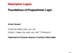
to clarify the intuition behind each of them. For example, ¬ℑ ϕ implies that ϕ does not hold in the first in-scope state encountered. ϕ Uℑ ψ means that ϕ holds in all the in-scope states preceding the one in which ψ holds. Xℑ ϕ means that ϕ holds in the next in-scope state after the first such state encountered, and if no in-scope states exist along the path, the property will not hold. Fℑ ϕ means that ϕ eventually holds in an in-scope state irrespective of its validity in out-of-scope states. Similarly, Gℑ ϕ means that ϕ holds in all the in-scope states on the path. Figure 1 illustrates several simple properties with ℑ-scope states. Definition 2. Let ℑ be a propositional logic expression, the operators ¬ℑ, ∧ℑ, Uℑ, Xℑ, Fℑ, and Gℑ are as follows: def

1.

¬ℑ ϕ = ¬ ℑ U (¬ϕ ∧ ℑ)

2.

∧ℑ ψ = ¬ℑ U ((ϕ ∧ψ) ∧ ℑ)

3.

ϕ Uℑ ψ = (ℑ → ϕ) U (ψ ∧ ℑ)

4.

Xℑ ϕ = ¬ℑ U [ℑ ∧ X (¬ℑ U (ℑ ∧ ϕ))]

5.

Fℑ ϕ = F (ϕ ∧ ℑ)

6.

Gℑ ϕ = G (ℑ → ϕ)

def

def

def

(ϕ ∧ ψ) In ℑ = (ϕ In ℑ) ∧ℑ (ψ In ℑ) (ϕ U ψ) In ℑ = (ϕ In ℑ) Uℑ (ψ In ℑ) (G ϕ) In ℑ = Gℑ (ϕ In ℑ) (F ϕ) In ℑ = Fℑ (ϕ In ℑ) (X ϕ) In ℑ = Xℑ (ϕ In ℑ)

The following lemmas and theorems describe the semantics of the introduced operators. Lemma 1. π ⊨ p In ℑ ⇔ there exists an i, 0 ≤ i < |π|, such that πi ⊨ p and πi ⊨ ℑ, and for all j, 0 ≤ j < i, πj ⊭ ℑ. Proof. π ⊨ p In ℑ ⇔ (According to the definition of p In ℑ), π ⊨ ¬ℑ U (p ∧ ℑ). ⇔ (By semantics of U), there exists an i, 0 ≤ i < |π| such that πi ⊨ (p ∧ ℑ) and for all j, 0 ≤ j < i, πj ⊨(¬ℑ), and (by semantics of ∧) πi ⊨ p and πi ⊨ ℑ, (by semantics of ¬) πj ⊭ ℑ. ⇔ There exists an i, 1 ≤ i < |π| such that πi ⊨ p and πi ⊨ ℑ, and for all j, 0 ≤ j < i, πj ⊭ ℑ. QED Lemma 2. π ⊨ ¬ℑ ϕ ⇔ there exists an i, 0 ≤ i < |π|, such that πi ⊭ ϕ and πi ⊨ ℑ, and for all j, 0 ≤ j < i, πj ⊭ ℑ. Proof. Lemma 2 directly follows from Lemma 1. QED

def

def

Based on these auxiliary definitions, we introduce the ℑscope operator denoted In, with the following recursive definition.

ℑ

ℑ

ϕ

ϕ

ℑ

ϕU Uψ ψ ℑ

ϕ

ψ

ℑ

Xϕ ϕ

3. 4. 5. 6. 7.

ϕ

ϕ ℑ

Fϕ ϕ

ϕ

ϕ

ℑ

ℑ

ℑ

ℑ

ϕ

ϕ

ϕ

ϕ

Gϕ

Fig. 1. Examples of properties using ℑ-scope operators.

Definition 3. Let ℑ be a propositional logic expression, the ℑ-scope operator In is defined as follows: 1. p In ℑ = ¬ℑ U (p ∧ ℑ) 2. (¬ϕ) In ℑ = ¬ℑ (ϕ In ℑ)

Lemma 3. π ⊨ ϕ Uℑ ψ ⇔ there exists an i, 0 ≤ i < |π|, such that πi ⊨ ψ and πi ⊨ ℑ, and for all j, 0 ≤ j < i πj ⊭ ℑ or πj ⊨ ϕ. Proof. π ⊨ ϕ Uℑ ψ ⇔ (According to definition of Uℑ), π ⊨ (ℑ → ϕ) U (ψ ∧ ℑ). ⇔ (By semantics of U), there exists an i, 0 ≤ i < |π| such that πi ⊨ (ψ ∧ ℑ) and for all j, 0 ≤ j < i, πj ⊨ (ℑ → ϕ); and (by semantics of ∧), πi ⊨ ψ and πi ⊨ ℑ, and (by definition of →), ℑ → ϕ = ¬ ℑ ∨ ϕ, and (by semantics of ¬ and ∨) πj ⊭ ℑ or πj ⊨ ϕ. ⇔ There exists an i, 0 ≤ i < |π| such that πi ⊨ ψ and πi ⊨ ℑ, and for all j, 0 ≤ j < i, πj ⊭ ℑ or πj ⊨ ϕ. QED Lemma 4. π ⊨ Xℑ ϕ ⇔ there exist i, k, 0 ≤ i < k ≤ |π|, such that πi ⊨ ℑ, πk ⊨ ℑ and πk ⊨ ϕ, and for all j, l, 0 ≤ j < i < l < k, πj ⊭ ℑ and πl ⊭ ℑ. Proof. π ⊨ Xℑ ϕ ⇔ π ⊨ ¬ℑ U [ℑ ∧ X (¬ℑ U (ℑ ∧ ϕ))]. ⇔ (According to semantics of U), there exists an i, 0 ≤ i < |π| such that πi ⊨ [ℑ ∧ X (¬ℑ U (ℑ ∧ ϕ))] and for all j, 0 ≤ j < i, πj ⊨ ¬ ℑ; and (by semantics of ∧), πi ⊨ ℑ and πi ⊨ X (¬ℑ U (ℑ ∧ ϕ)), and (by semantics of X), πi+1 ⊨ (¬ℑ U (ℑ ∧ ϕ)); and (by semantics of U), there exists k, i + 1 ≤ k < |π| such that πk ⊨(ℑ ∧ ϕ) and for all l, i < l < k, πl ⊨ ¬ℑ.

⇔ There exist i, k, 0 ≤ i < k < |π|, such that πi ⊨ ℑ, πk ⊨ ℑ and πk ⊨ ϕ, and for all j, l, 0 ≤ j < i < l < k, πj ⊭ ℑ, and πl ⊭ ℑ. QED Lemma 5. π ⊨ Fℑ ϕ ⇔ for some i, 0 ≤ i < |π|, πi ⊨ ϕ and πi ⊨ ℑ. Proof. Directly follows from the semantics of F. QED Lemma 6. π ⊨ Gℑ ϕ ⇔ for all i, 0 ≤ i < |π|, where πi ⊨ ℑ, πi ⊨ ϕ. Proof. Directly follows from the semantics of G. QED To demonstrate the correctness of the proposed operators and formulae, we state two theorems in which we claim that if a formula (ϕ In ℑ) holds in a given path (model) including inscope and out-of-scope states the corresponding LTL formula ϕ must hold in the projection of the path (model) including only the in-scope states. To this end, we first define a projection relation based on Definition 1 that removes the outof-scope states from a path and keeps only the in-scope states. Definition 4. Let ℑ be a propositional logic formula, M = (S, T, S0, L) be a Kripke structure, Sℑ = {s ∈ S | ℑ is true in s}, and let π = 〈s0, s1, …〉 be a path of M. The projection of π onto Sℑ, denoted π↓ℑ, is the (possibly finite) subsequence of π derived by discarding all states si from π such that si ∉ Sℑ. Proposition 1. Let ℑ be a propositional logic formula, and M = (S, T, S0, L) and Mℑ = (Sℑ, Tℑ, S0ℑ, Lℑ) be two Kripke structures, where Mℑ is the projection of M onto Sℑ, and π be a path of M, then π↓ℑ ≠ ε is a path of Mℑ. The following theorem states that if a formula with the scope operator holds on a path, then the corresponding formula with no scope operator must hold on the projection of the path onto the designated scope. Theorem 1. For any LTL formula ϕ and its corresponding formula ϕ In ℑ, π ⊨ ϕ In ℑ if and only if π↓ℑ ⊨ ϕ. Proof. The proof is by induction on the number of operators, n, of a formula ϕ. For simplicity, we assume that ℑ is an atomic proposition. The proof could easily be extended onto any propositional ℑ. To make the proof more intuitive, we index the formulae with the number of operators that constitute each formula. Base case. For n = 0, where the formula is simply an atomic predicate and ϕ0 In ℑ = p In ℑ, we prove that π ⊨ p In ℑ if and only if π↓ℑ ⊨ p.

π ⊨ p In ℑ ⇔ π ⊨ ¬ ℑ U (p ∧ ℑ). ⇔ (According to Lemma 1) there exists an i, 0 ≤ i < |π|, such that πi ⊨ p and πi ⊨ ℑ, and for all j, 0 ≤ j < i, πj ⊭ ℑ. ⇔ There exists an i, 0 ≤ i < |π|, such that p ∈ L(si) and ℑ ∈ L(si), and for all j, 0 ≤ j < i, ℑ ∉ L(sj); and (by Definition 4) si is the first state in πi↓ℑ and for all j, 0 ≤ j < i, sj is not in πj↓ℑ . ⇔ There exists an i, 0 ≤ i < |π|, such that π = 〈…, si, …〉, πi↓ℑ ⊨ p and π↓ℑ = πi↓ℑ = 〈si, …〉. ⇔ (According to the semantics of p) π↓ℑ ⊨ p. Inductive step. Assume π ⊨ ϕm In ℑ if and only if π↓ℑ ⊨ ϕm holds for all formulae ϕm that consist of m operators, where 0 ≤ m ≤ n. We must show that the equivalence holds as well for n + 1. We present here the proofs only for the most complicated cases where the formula ϕn+1 is of the form χu U ψv, where χu and ψv are formulae with u and v operators respectively, such that, 0 ≤ u ≤ n, 0 ≤ v ≤ n, and u + v = n, and of the form X ψn. The proofs for the remaining LTL operators could be performed in a similar manner. (1) Here we prove that for all formulae χu, ψv which together contain n or less operators, π ⊨ (χu U ψv) In ℑ if and only if π↓ℑ ⊨ χu U ψv. π ⊨ (χu U ψv) In ℑ ⇔ π ⊨ (χu In ℑ) Uℑ (ψv In ℑ). ⇔ (According to Lemma 3) there exists an i, 0 ≤ i < |π|, such that πi ⊨ (ψv In ℑ) and πi ⊨ ℑ, and for all j, 0 ≤ j < i πj ⊭ ℑ or πj ⊨ (χu In ℑ). ⇔ There exists an i, 0 ≤ i < |π|, such that (by Definition 4) si is the first state in πi↓ℑ, and (according to the induction hypothesis) for all i, 0 ≤ i < |π|, πi↓ℑ ⊨ ψv; and for all j, 0 ≤ j < i, either (by Definition 4) sj is not in πj↓ℑ, or sj is a state in πj↓ℑ and (by induction hypothesis) πj↓ℑ ⊨ χu. ⇔ There exists an i, 0 ≤ i < |π|, such that π = 〈…, si, …〉, (πi↓ℑ ⊨ ψm, and π↓ℑ = πi↓ℑ = 〈si, …〉) or (πi↓ℑ ⊨ ψv, and for all j, 0 ≤ j < i, πj↓ℑ ⊨ χu). ⇔ (By semantics of U) π↓ℑ ⊨ χu U ψv. (2) Here we prove that for each formula ψn that contain n or less operators, π ⊨ (X ψn) In ℑ if and only if π↓ℑ ⊨ X ψn. π ⊨ (X ψn) In ℑ ⇔ Xℑ (ψn In ℑ). ⇔ (According to Lemma 4) there exist i, k, 0 ≤ i < k < |π|, such that πi ⊨ ℑ, πk ⊨ ℑ and πk ⊨ (ψn In ℑ), and for all j, l, 0 ≤ j < i < l < k, πj ⊭ ℑ, and πl ⊭ ℑ.

⇔ There exist i, k, 0 ≤ i < k < |π|, such that ℑ ∈ L(si), ℑ ∈ L(sk), and πk ⊨ (ψn In ℑ), and for all j, 0 ≤ j < i, ℑ ∉ L(sj), and for all l, i+1 ≤ l < k, ℑ ∉ L(sl). ⇔ There exist i, k, 0 ≤ i < k < |π|, such that (by Definition 4) si is the first state in πi↓ℑ, sk is the first state in πk↓ℑ, such that (by induction hypothesis) πk↓ℑ ⊨ ψn, and for all j, 0 ≤ j < i, sj is not in πj↓ℑ, and for all l, i+1 ≤ l < k, sl is not in πl↓ℑ. ⇔ There exist i, k, 0 ≤ i < k < |π|, such that π = 〈…, si, …, sk, …〉, π↓ℑ = 〈si, sk, …〉, and πk↓ℑ ⊨ ψn. ⇔ (By semantics of X) π↓ℑ ⊨ X ψn. The base case and the induction step imply that the theorem holds for all cases of n. QED Given Proposition 1 and Theorem 1, we have the following theorem which states that if a formula with the scope operator holds in a Kripke, then the corresponding formula with no scope operator must hold on the projection of the Kripke onto the designated scope. Theorem 2. Let ℑ be a propositional logic formula, and let M = (S, T, S0, L) and Mℑ = (Sℑ, Tℑ, S0ℑ, Lℑ) be two Kripke structures, Mℑ is the projection of M onto Sℑ ⊆ S such that ℑ is true in all s ∈ Sℑ. For any LTL formula ϕ, M ⊨ ϕ In ℑ if and only if Mℑ ⊨ ϕ. Note that Definitions 2, and 3 are not the only possible way to express propositional scopes in LTL formulae. For example, we surmise that shorter formulae could be obtained with a longer list of rules that differentiate between temporal and propositional terms. Definition 3a. Let ϕ and ψ be arbitrary LTL formulae, p, q, and ℑ be a propositional logic expression, the ℑ-scope operator In is defined as follows: 1. p In ℑ = ¬ℑ U (p ∧ ℑ) 2. (¬ϕ) In ℑ = ¬ℑ (ϕ In ℑ) 3. (p ∧ q) In ℑ = p ∧ℑ q 4. (p U q) In ℑ = p Uℑ q 5. (G p) In ℑ = Gℑ p 6. (F p) In ℑ = Fℑ p 7. (ϕ ∧ ψ) In ℑ = (ϕ In ℑ) ∧ℑ (ψ In ℑ) 8. (ϕ U ψ) In ℑ = (ϕ In ℑ) Uℑ (ψ In ℑ) 9. (G ϕ) In ℑ = Gℑ (ϕ In ℑ) 10. (F ϕ) In ℑ = Fℑ (ϕ In ℑ) 11. (X ϕ) In ℑ = ¬ℑ U (ℑ ∧ X (ϕ In ℑ)) Translation into automata could be even more efficient, though not all verification tools allow direct specification of properties in automata.

IV. EXAMPLE This work is primarily motivated with the analysis and verification of various applications where natural distinctions between states arise. Still we believe that the suggested operators are useful in many other areas, which go even beyond verification and testing. We illustrate the effectiveness of the defined operators with an example commonly used in automated planning [28], where model checking is increasingly applied. The system is the so-called Dock-Worker Robots or DWR domain, which represents a harbor with several locations corresponding to docks, docked ships, storage areas, etc [28]. In the harbor, robot carts are used in the loading and unloading of docked ships. In this example, we consider a property that expresses a desired robot behavior. Robot1 visits Room1 then Room2 then returns to Room1 and does this exactly twice. In this property, Robot1 is assumed to start in Room1 while the rooms are adjacent. We generalize the property to express a more realistic situation, assuming that the robot can start in any location and the two rooms are not adjacent (they are interleaved with other locations where the robot is allowed to pass). Therefore, given the stated property, we are not interested in the robot movement in any other locations other than Room1 and Room2. Using standard LTL, the generalized property is non-trivial and tricky to specify: (¬Room1 ∧ ¬Room2) U (Room1 ∧ ¬Room2 ∧ X (¬Room2 U (Room2 ∧ ¬Room1 ∧ X (¬Room1 U (Room1 ∧ ¬Room2 ∧ X (¬Room2 U (Room2 ∧ ¬Room1 ∧ X (¬Room1 U (Room1 ∧ ¬Room2 ∧ X (G (¬Room2))))))))))) (1) If we use now the In operator, the scope of the property includes states where the robot can be in Room1 or in Room2. Therefore, the scope can be written as: (Room1 + Room2). Note that exclusive disjunction is used to account for a situation when the robot cart or train did not completely leave one location, while entering in another one. In the case when both locations are adjacent, the robot could be stuck between two locations instead of performing a repetitive movement. Now, the property can be written, in a more intuitive and succinct way, with the In operator as follows: Room1 ∧ X(Room2 ∧ X(Room1 ∧ X(Room2 ∧ X(Room1 ∧ G(¬Room2))))) In (Room1 + Room2) (2) We leave the task of unfolding the formula in (2) and comparing the result to (1) as an exercise for the reader.

V. USING ℑ-SCOPE IN PROPERTY PATTERNS Using scopes to limit the domain over which a property is verified was only recently addressed in [7, 8] by Dwyer et al. The authors identify several scopes which are used to define the part of a system execution, where a property must hold. A scope is determined by specifying starting and ending state/event for the property. The defined scopes are then used within a system of property specification patterns that are useful for non-experts to read and write formal specifications of systems. We believe that the ℑ-scope, when combined with the existing scope definitions, provides a possibility to further enrich the expressiveness of patterns and make them more useful in practice. A. System of Property Patterns In [7, 8], patterns are classified into two categories: Order and Occurrence, and they include: - Absence - A given state/event does not occur within a scope; - Existence - A given state/event must occur within a scope; - Universality - A state/event occurs throughout a scope; - Response - A state/event P must be always followed by a state/event Q within a scope; - Precedence - A state/event P must be always preceded by a state/event Q within a scope.

Global

-

After - The execution path after a given state/event; Between - Any part of the execution path from one given state/event to another given state/event; After-until - Similar to scope Between, except that the designated part of the execution path continues even if the second state/event does not occur.

B. Combining ℑ-Scope with Pattern Scopes In this section, we show how the defined ℑ-scope can be combined with the pattern scopes introduced in [7,8] to provide the user of the pattern system with more flexibility to specify real world properties. For example, given the existence pattern in the global scope, we can verify it also in some states of interest defined by a given propositional logic expression ℑ. Thus the pattern becomes “Exist Globally in ℑ-scope states” and the corresponding LTL formula is: F (P ∧ ℑ).

Global |ℑ

ℑ

ℑ

ℑ

ℑ

ℑℑ

ℑ

R

ℑ ℑ Q

ℑℑ R

ℑ ℑ ℑ Q R

ℑ ℑ Q

ℑ

ℑ ℑ ℑ

ℑ

Q Before Q | ℑ

ℑ

After R | ℑ

Q Between Q and R | ℑ

After Af ter Q until R | ℑ

ℑ R

Q ℑ R

ℑ

ℑ R Q ℑ ℑ ℑ

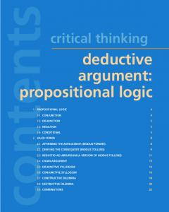
Before Q Fig. 3. New Scopes

After R

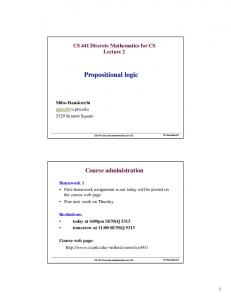
Figure 3 shows the combination of the original scopes (represented in light gray) and the ℑ-scope. The resulting scopes are shown using dark gray rectangles.

Between Q and R

After Q until R

Fig. 2. Pattern Scopes

In addition, there are five scopes (Figure 2) that can be associated to patterns: - Global - The entire execution path; - Before - The execution path up to a given state/event;

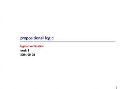
Consequently, we introduce LTL templates for the specification patterns with the modified scopes. These templates can be loaded into the LTL Property Manager of Spin where the propositional expression of the scope can be instantiated in the macro definition of the scope within the templates as needed by the user. Figures 4, 5, and 6 show examples of the new scopes applied to the patterns Absence, Existence, and Precedence. Figures 7 and 8 show some of the resulting templates. Note that new patterns are obtained by rewriting the old

patterns using the operator In and the proposition ℑ, and unfolding and simplifying the resulting formulae.

Absence pattern: P is False

Precedence pattern: S precedes P

Globally in ℑ-scope states: G (ℑ → ¬P)

Globally in ℑ-scope states: (ℑ → ¬P) W (ℑ ∧ S)

Before R in ℑ-scope states: F (R ∧ ℑ) → (ℑ → ¬P) U (R ∧ℑ)

Before R in ℑ-scope states: F(ℑ ∧ R) → (ℑ → ¬P) U (ℑ ∧ (S | R))

After Q in ℑ-scope states: G ((ℑ → Q) → G (ℑ → ¬P))

After Q in ℑ-scope states: G (ℑ → ¬Q) | F (ℑ ∧ Q ∧ (ℑ → ¬P) W (ℑ ∧ S))

Between Q and R in ℑ-scope states: G ((ℑ → Q ∧ ¬R ∧ F (R ∧ ℑ)) → (ℑ → ¬P) U (ℑ ∧ R))

Between Q and R in ℑ-scope states: G ((ℑ → Q ∧ ¬R ∧ F (R ∧ ℑ)) → (ℑ → ¬P) U (ℑ ∧ (S | R)))

After Q until R in ℑ-scope states: G ((ℑ → Q ∧ ¬R) → (ℑ → ¬P) W (ℑ ∧ R))

After Q until R in ℑ-scope states: G ((ℑ → Q ∧ ¬R) → (ℑ → ¬P) W (ℑ ∧ (S | R)))

Fig. 4. Absence Pattern with new Combined Scopes

Existence pattern: P becomes True Globally in ℑ-scope states: F (P ∧ ℑ) Before R in ℑ-scope states: (ℑ → ¬R) U ((ℑ ∧ P ∧ ¬R) | (ℑ → ¬R)) After Q in ℑ-scope states: G (ℑ → ¬Q) | F (ℑ ∧ Q ∧ F (ℑ ∧ P)) Between Q and R in ℑ-scope states: G ((ℑ → Q ∧ ¬R) → (ℑ → ¬R) W (ℑ ∧ P ∧ ¬R)) After Q until R in ℑ-scope states: G ((ℑ → Q ∧ ¬R) → (ℑ → ¬R) U (P ∧ ¬R ∧ ℑ))

Fig. 6. Precedence Pattern with new Combined Scopes

##define define p ? # define i ? /* * Formula As Typed : (p && i) * The Never Claim Below Corresponds * To The Negated Formula !( (p && i)) * ( formalizing violations of the * original) */ never { /* !( (p && i)) */ accept_init : T0_init: if :: ((! ((i )) || !((p)))) -> goto T0_init fi; }

Fig. 7. Templates for Existence pattern Globally in ℑ-scope Fig. 5. Existence Pattern with new Combined Scopes

In the future, we may consider temporal extension of the proposed scope operator, which will allow the application of not only propositional, but also the above mentioned temporal scopes, to arbitrary formulae, possibly in an iterative manner.

#define p ? #define i ? #define r ? /* * Formula As Typed: (i -> ! r) U ((i && p * && ! r) || (i -> ! r)) * The Never Claim Below Corresponds * To The Negated Formula !((i -> ! r) U ((i * && p && ! r) || (i -> ! r))) * (formalizing violations of the original) */ never { /* !((i -> ! r) U ((i && p && ! r) || (i -> ! r)))" */ accept_init: T0_init: if :: ((i) && (r)) -> goto T0_init :: ((i) && (r)) -> goto accept_all fi; accept_all: skip } Fig. 8. Templates for Existence pattern Before R in ℑ-scope

VI. RELATED AND FUTURE WORK In logic theory scope imposing is known as relativization, and is used for producing inner models of set theory. Relativisation was also addressed in dynamic epistemic logic, which is equivalent in expressive power to modal logic. These results are used for public communications in the context of multi-agent systems [30]. Manna and Wolper [29] propose the so-called relativization rules in the context of synthesis of communicating processes. Relativisation takes a PTL specification of a single process and transforms it into a specification of the global system. There are certain similarities between these rules and our work. However, there are two main differences between the approaches. First, the relativization procedure they propose applies only on infinite scopes, while our definitions equally apply to both finite and infinite scopes and models. The second difference is that the relativization transformations [29] apply when the atomic propositions of a given formula hold only in the scope, while we do not make any assumptions on dependencies between the property and the scope. There exist also several works on introducing and/or extending specification logics based on existing ones, such as LTL and CTL, to ease the expression of properties of systems or allow a wider range of specifications to be expressed using these logics. Examples of such logics are QCTL [15], an extension of CTL with quantification over propositional

formulae, XCTL [3], an extension of CTL to De Morgan Algebras, and DLTL [12], a logic that extends LTL by indexing the until operator with regular programs. The most recent work we know about is the one of Chaki et al [2]. The authors introduce a framework for modeling and verification of concurrent software systems, where both states and events are incorporated. For this purpose, they introduce SE-LTL, a specification logic based on LTL that allows both state and event requirements to be easily expressed. Beer et al [1] propose the so-called Temporal Logic Sugar. They extend CTL with regular expressions and introduce new operators to formulate properties in CTL. These operators do not add expressive power to CTL, but make it easier for the non-expert user of CTL to specify properties of interest. The operator "next" defined in Sugar is close to the "next in scope" operator we provide, but our definition is more general. The Sugar next is defined as the next state in which a Boolean expression is valid. Our definition states that the property has to be true in the next state, in which a propositional logic expression is valid, relatively to the first state in which the propositional logic expression is valid and not to the first state of the execution path. Dwyer et al [7, 8] present and analyze over 500 temporal properties, classified in the proposed specification pattern system [26]. The patterns introduced constitute abstractions of specifications formulated for different formalisms in which such abstractions are not supported. The patterns are defined on five scopes that represent intervals/regions in which properties should be validated. These scopes have a start state and an end state. However, the authors did not address the problem of specifying these patterns in a scope of arbitrary set of states. Although the authors mention a class of properties that could be defined based on Boolean variables true in a state, but they state that the specification of these properties is not trivial and offer no solution to this problem. Moreover, there is no methodology to impose those scopes on a given pattern/formula. Since the specification pattern system does not use automatic combinations of scopes and basic patterns, some attempts are made to translate the system to lower-level automata specification languages. Such translations make pattern visualization, fiddling, and elucidation [10, 21] possible. Chechik et al [4, 17] extend the pattern system of [7, 8] and introduce edge based LTL property formulations in the same scopes introduced by Dwyer. The notion of an edge/event is represented by the "next" operator. Dillon et al [6] introduce in the Graphical Interval logic (GIL) which is similar to the pattern system.

GIL provides a mechanism to identify the region/interval of the system execution over which the property should be validated. The operators that identify the intervals introduce a wider and more general range of scopes than the five scopes introduced by Dwyer. However, the operators are used to define segments of the execution path that must have a start and an end. There is no means offered to identify an arbitrary set of states in which properties should be verified. Currently, we are working on extending our idea toward temporal scopes and studying properties of the resulting logics. However, we need to perform more case studies to justify the extension toward temporal scopes. Possibly, this work could contribute to the improvement and elucidation of existing specification patterns, e.g., in relation to mixed open/closed delimiters, mixed state/event properties etc. Generalizing our approach to introduce temporal scopes provides a richer and more flexible framework and methodology that could allow for automated, possibly recursive application of temporal scopes, such as described in existing pattern repositories [7, 8], to various formulae. For example, the pattern globally P after Q until R could be stated as G P In (¬R S Q), where S is the “past time” LTL operator since, that could be translated back [31] into the usual “future time” LTL, though the transformation is not elementary. However, it is not yet clear whether In operator could be used for all the scopes and properties of interest. Allowing temporal scopes introduces several issues that need to deal with. First, we intend to develop algorithms and tools for translation of formulas with In operator into automata. Another option is to develop a tool that translates any given LTL property that includes scope operators into standard LTL and applies optimization and simplification rules on the resulting LTL formula. While transformation into automata could be more practical and convenient for users of tools that support automata properties/observers, such as Spin never claims or Object Geode Goal, there are tools, such as NuSMV, that support LTL, but not observers. Second, using temporal scopes, we designate the states of interest with a temporal formula. This can save us from introducing designated predicates and variables distinguishing states in scope from the others, e.g., transient and stable states of the system. Formal investigation of the impact of the proposed operators on succinctness and complexity of logics could be of certain theoretical and practical value.

VII. CONCLUSION In this paper, we defined new specialized LTL operators that assess in the specification of properties within a scope of arbitrary set of states of interest. A propositional logic formula ℑ characterizes these states which constitute what we call ℑscope. These defined operators do not extend the LTL formalism; they rather help formulate complex specifications more intuitively and succinctly. Therefore, these operators do not require designated model checking algorithms. The new operators could be used to easily specify properties of the systems, particularly, in the case when some states of a system are of technical character and should be skipped. We believe that the proposed operators can be used in models that exhibit both infinite and finite behaviors, and are useful, in various application domains. While we have not presented any tools to support the proposed operators yet, we extend the existing specification pattern system, which embraces most used property patterns, with additional propositional scopes.

ACKNOWLEDGMENT The first author acknowledges stimulating communications with Gerard Holzmann.

REFERENCES [1] I. Beer, S. Ben-David, and C. Eisner, “The Temporal Logic Sugar” in Proc. of 13th Int. Conference on Computer Aided Verification (CAV 2001), LNCS, Vol. 2102, pp. 363–367. [2] S. Chaki, E.M. Clarke, and J. Ouaknine, N. Sharygina, N. Sinha, “State/Event-based Software Model Checking”, in Proc. of 4th Int. Conference on Integrated Formal Methods (IFM 04), LNCS, Vol. 2999. Canterbury, England, April 2004. [3] M. Chechik, B. Devereux, S. Easterbrook, and A. Gurfinkel, “Multi-valued Symbolic Model-Checking” ACM Transactions on Software Engineering and Methodology (TOSEM), Vol. 12 , Issue 4, pp. 371 – 408, October 2003. [4] M. Chechik, and D. Paun, “Events in Property Patterns”, in Proc. of 6th Int. SPIN Workshop on Theoretical and Practical Aspects of SPIN Model Checking, LNCS 1680, pp. 154-167, September 1999. [5] M. Clarke, O. Grumberg, D. A. Peled, Model Checking. MIT Press, 2000. [6] L.K. Dillon, G. Kutty, L.E. Moser, “A Graphical Interval Logic for Specifying Concurrent Systems”, ACM Transactions on Software Engineering and Methodology, Vol. 3(2), pp. 131-165, April 1994. [7] M. Dwyer, G.S. Avrunin, and J.C. Corbett, “Patterns in Property Specifications for Finite-state Verification”, in Proc. of 21st Int. Conference on Software Engineering, May, 1999. [8] M. Dwyer, G.S. Avrunin, and J.C. Corbett, “Property Specification Patterns for Finite-state Verification”, in Proc.

[9] [10]

[11]

[12] [13] [14] [15] [16] [17] [18]

[19] [20]

[21]

[22] [23]

[24] [25] [26]

of 2nd Workshop on Formal Methods in Software Practice, March, 1998. E. Emerson, and J. Halpern, “ ‘sometimes’ and ‘not never’ Revisited: on Branching versus Linear Temporal Logic”, Journal of the ACM, 33(1), pp. 151-178, January 1986. H. Hallal, A. Petrenko, A. Ulrich, and S. Boroday, “Using SDL Tools to Test Properties of Distributed Systems”, in Proc. of Formal Approches to Testing of Software (FATES’01), Workshop of the Int. Conference on Concurrency Theory (CONCUR’01). pp. 125-140, Aalborg, Denmark, August 21-24, 2001. M. Haydar, A. Petrenko, and H. Sahraoui, “Formal Verification of Web Applications Modeled by Communicating Automata”, in Proc. of 24th IFIP WG 6.1 IFIP Int. Conference on Formal Techniques for Networked and Distributed Systems (FORTE 2004), LNCS, Vol. 3235, pp. 115-132, Spain, September 2004. J.G. Henriksen, and P.S. Thiagarajan, “Dynamic Linear Time Temporal Logic”, in Annals of Pure and Applied logic, Vol.96, No.1-3, pp. 187–207, 1999. G.J. Holzmann, The Spin Model Checker, Primer and Reference Manual. Addison-Wesley, 2003. M.R.A. Huth, and M.D. Ryan, Logic in Computer Science: Modelling and Reasoning about Systems. Cambridge University Press, 2000. O. Kupferman, “Augmenting branching temporal logics with existential quantification over atomic propositions”, Journal of Logic and Computation, Vol. 9(2), p. 135-147, April 1999. L. Lamport, “Sometimes is sometimes ‘not never’ ”, in Proc. of 7th ACM Symposium on Principles of Programming Languages, pp. 174-185, January 1980. D. Paun, and M. Chechick, “Events in Linear-Time Properties”, in Proc. of 4th IEEE Int. Symposium on Requirements Engineering, June 1999. A. Petrenko, N. Yevtushenko, G.v. Bochmann, and R. Dssouli, “Testing in Context: Framework and Test Derivation”, Computer Communications Journal, Special issue on Protocol engineering, Vol. 19, pp. 1236-1249, 1996. A. Pnueli, “The Temporal Logic of Programs”, in Proc. of the 18th IEEE Symposium on Foundations of Computer Science, 1977, pp. 46-57. M.H. Smith, G.J. Holzmann, and K. Etessami, “Events and Constraints: a Graphical Editor for Capturing Logic Properties of Programs”, in Proc. of the 5th Int. Symposium on Requirements Engineering, August 2001. R.L. Smith, G.S. Avrunin, L.A. Clarke, L.J. Osterweil, “PROPEL: an Approach Supporting Property Elucidation”, in Proc. of 24th Int. Conference on Software Engineering (ICSE 2002), pp. 11 – 21, Orlando, Florida, 2002. J. Tretmans, “Test Generation with Inputs, Outputs and Repetitive Quiescence”, Software-Concepts and Tools, Vol.3, pp. 103-120, 1996. M.Y. Vardi, “Branching vs. Linear Time: Final Showdown”, in Proc. of the 7th Int. Conference on Tools and Algorithms for the Construction and Analysis of Systems (TACAS 2001), LNCS, Vol. 2031 pp. 1–22, Italy, April 2001. C.H. West, “An Automated Technique of Communication Protocols Validation”, IEEE Transactions on Communication. Vol. 26, pp. 1271-1275, 1978. Mathworld, The Web’s most Extensive Mathematics Resource [Online]. Available:http://mathworld.wolfram.com/. The Specification Patterns System [Online]. Available: http://patterns.projects.cis.ksu.edu/.

[27] H. Barringer, A. Goldberg, K. Havelund, and K. Sen, “Eagle Does Space Efficient LTL Monitoring”, Technical Report, CSPP-25, University of Manchester, Department of Computer Science, October 2003. [28] M. Ghallab, D. Nau, and P. Traverso, Automated Planning: Theory and Practice. Morgan Kaufmann Publishers, May 2004. [29] Z. Manna, and P. Wolper, “Synthesis of Communicating Processes from Temporal Logic Specifications”, in ACM Transactions on Programming Languages and Systems, Vol. 6, No. 1, January 1984, pp. 68-93. [30] J. Plaza, “Logics of Public Communications”, in Proc. of the 4th International Symposium on Methodologies for Intelligent Systems (M.L. Emrich, M.S. Pfeifer, M. Hadzikadic, Z.W. Ras, eds.), North-Holland, 1989, pp. 201-216. [31] D. Gabbay, A. Pnueli, S. Shelah, and J. Stavi, “On the Temporal Analysis of Fairness”, in Proc. of the 7th ASM Symposium on Principles of Programming Languages (POPL'80), pp. 163-173. ACM Press, January 1980.