Proscriptive Bayesian Programming Application for Collision Avoidance Carla Koike† , C´edric Pradalier, Pierre Bessi`ere, Emmanuel Mazer GRAVIR-INRIA-INPG Grenoble, France
[email protected],
[email protected] [email protected],
[email protected] †Corresponding Author: INRIA Rhˆ one-Alpes, 38334 Saint Ismier cedex France
Abstract— Evolve safely in an unchanged environment and possibly following an optimal trajectory is one big challenge presented by situated robotics research field. Collision avoidance is a basic security requirement and this paper proposes a solution based on a probabilistic approach called Bayesian Programming. This approach aims to deal with the uncertainty, imprecision and incompleteness of the information handled. Some examples illustrate the process of embodying the programmer preliminary knowledge into a Bayesian program and experimental results of these examples implementation in an electrical vehicle are described and commented. Some videos illustrating these experiments can be found at http://www-laplace.imag.fr.
I. I NTRODUCTION When expected to evolve safely in an unaffected environment, a mobile robot shall execute its tasks avoiding contact with obstacles, if possible following an optimal trajectory during displacements. Specially in the context of vehicles, the presence of several obstacles at the same time can remarkably increase the complexity of signal processing and turn the obstacle avoidance unfeasible. Depending on the sensors technology some characteristics as size, distance, color and even texture of obstacle surface can change the precision and reliability of the avoidance method. One way to approach this complexity is to deal with the uncertainty in the avoidance reasoning, trying to express the imprecision and incompleteness of information handled. This paper describes a probabilistic approach and how it can be used to solve the obstacle avoidance problem. Probabilities will be used to express uncertainty, and to express knowledge specific to obstacle avoidance, in the context of bayesian programming. The rest of this paper is organized as follows. First, a very short review of methods for obstacle avoidance is presented in section II, while in section III, the Bayesian Programming Approach is briefly described. Section IV addresses different methods employed to solve the obstacle avoidance problem with Bayesian Programming and each proposed solution is illustrated with results and comments.
II. O BSTACLE AVOIDANCE R ELATED W ORK In situated robotics, it is desired to have the robot evolving in non adapted and populated environment, requiring collision-free motion and fast reaction to unexpected events. This section presents a brief description of methods commonly used in obstacle avoidance in robotics. Potential field methods ([6] and [11]) try to solve the navigation problem as function optimization: find the necessary commands to bring the robot in the global minimum value of a function that decreases near the target position and increases away from the target and near the obstacles. Steering Angle Field Method, proposed by Feiten et al in 1994 [3], uses the curvature tangent to obstacle to constrain the continuous space of steering angles. The dynamic window approach ([4] and [5]) proposes to avoid the obstacles by searching in the velocities space in order to maximize an objective function, whose terms include the measure of the progress toward the target position, the position of the nearest obstacles and the forward velocity of the robot. In the specific situation of dynamic obstacles some particular methods were conceived [7]. When the trajectories are known a-priori, global approachs are usually considered. But in the general case these trajectories are not known and have to be infered from current observations: obstacle avoidance being performed in reaction to these previsions, local approach methods are more suitable. Some probabilistic approachs [10] for navigation use Markov Decision Processes (MDPs) for finding the optimal admissible control command that leads the robot to the goal, avoiding obstacles. III. BAYESIAN P ROGRAMMING When programming a robot, the programmer builds an abstract representation of its environment, which is basically composed of geometric, analytic and symbolic notions. In a way, the programmer imposes on the robot his or her own abstract conception of the environment, supposing that the environment can be fully described by the abstract concepts used.
Due to the irreducible incompleteness of the model, it is not always easy to link these abstract concepts with the robot’s raw signals (either obtained from the robot’s sensors or being sent to the robot’s actuators). Controlling the environment is the usual answer to these difficulties, but it may not be desirable or possible when the robot must act in an environment not specifically designed for it, populated, or subject to unexpected and unattended events. Probabilistic methodologies and techniques offer possible solutions to the incompleteness and uncertainty difficulties when programming a robot. The basic programming resources are probability distributions, which are generated placing side by side the programmer’s conception task (actually, the expression of his or her preliminary knowledge about the robot, the environment and the task) and experimental data obtained from the environment. The Bayesian Programming approach was originally proposed as a tool for robotic programming (see [8] for a detailled description), but nowadays used in a wider scope of applications ( [2] and [9] show some examples).
found in [8]. They are the basis for the definition of a generic formalism to specify probabilistic models called Bayesian Programs. The elements of a Bayesian Program are briefly outlined in the rest of this section and they are illustrated in figure 2(a). A. Description The purpose of a description is to specify an effective method to compute a joint distribution on a set of relevant variables {X 1 , X 2 , . . . , X n }, given a set of experimental data δ and a preliminary knowledge π . In the specification phase of the description, it is necessary to: • Define a set of relevant variables {X 1 , X 2 , . . . , X n }, on which the joint distribution shall be defined; • Decompose the joint distribution into simpler terms, following the conjunction rule. Conditional independence hypotheses can allow further simplification, and such a simplified decomposition of the joint distribution is called decomposition. • Define the forms for each term in the decomposition; i.e. each term is associated with either a parametric form, as a function, or to another Bayesian Program. B. Question Given a description P(X 1 X 2 . . . X n | δ π ), a question is obtained by partitioning the variables {X 1 , X 2 , . . . , X n } into three sets: Searched, Known and Unknown variables. A question is defined as the distribution P(Search | Known δ π ). In order to answer this question, the following general inference is used:
Fig. 1.
Bayesian Programming and other probabilistic approaches
In this approach, a probability distribution is associated with the uncertainty of a logical proposition value. The usual notion of a Logical Proposition (either true or false) and its operators (negation, conjunction and disjunction ) are used when defining a Discrete Variable. By definition, a Discrete Variable X is a set of logical propositions xi such that these propositions are mutually exclusive (for all i, j with i 6= j, xi ∧ x j is false) and exhaustive (at least one of these propositions xi is true). The probability distributions assigned to logical propositions are always defined according to some preliminary knowledge, identified as π : so P(xi | π ) gives the probability distribution of the variable X having the value xi , knowing π . Most of the time, probabilities will be manipulated using the conjunction rule, also known as Bayes rule: P(XY | π ) = P(X | π )P(Y | X π ) = P(Y | π )P(X | Y π ).
Most details about the inference postulates and rules for carrying out probabilistic reasoning in this context can be
P(Search | Known δ π ) =
∑Unknown P(Search Unknown Known) ∑Unknown,Search P(Search Unknown Known)
Depending on number of variables (and its discretization) and decomposition choice, this calculation may need a lot of computational time and turn out to be infeasible. Numerous techniques have already been proposed to achieve admissible computation time and a brief summary of the approximative approaches used in our research team for reducing calculation time can be found in [9]. In [1], one of these approximative methods is described in details. a) Bayesian Programs and other probabilistic approaches: Bayesian programs have been shown to be a generalization of most of the other probabilistic approaches [1] as in the figure 1. It means that all these probabilistic approaches may be reformulated following the Bayesian program formalism and thus easily compared with one another. For instance, Bayesian networks correspond to a description where one and only one variable may appear left of each probability distribution appearing in the decomposition. This restriction enables optimized inference algorithms for certain class of question.
(a) Fig. 2.
Relevant Variables: Φ ∈ {−5, 5}, |φ | = 11 V ∈ {0, 5}, |V | = 6 Di ∈ {0, 200}, |Di | = 201, i = 1, . . . , 8 Decomposition: P(V Φ ~D | π f 1 ) = P(V Φ | π f 1 ) ∏8i=1 P(Di | V Φ π f 1 ) Parametrical Forms: P(V Φ | π ) = Uniform; f 1 π P(D | V Φ i f 1 ) = P(Di | V Φ πi f ) Identification: A Priori Question: P(V Φ | ~D π f 1 )
Specification
Description
Program
Specification
Relevant Variables: Φi ∈ {−5, 5}, |Φ| = 11 Vi ∈ {0, 5}, |V | = 6 Di ∈ {0, 200}, |Di | = 201 Decomposition: P(Φi Vi Di | πi ) = P(Di | πi )P(Vi | Di πi )P(Φi | Di πi ) Parametrical Forms: P(Di | πi ) = Uniform; P(Vi | Di πi ) = Gµv (Di );σv (Di ) (Vi ); P(Φi | Di πi ) = GµΦ (Di );σΦ (Di ) (φi ). Identification: A Priori Question: P(Di | V Φ πi )
Description
Program
(b)
Bayesian programs for behavior combination: a) Zone program b) Prescriptive Fusion Program
IV. O BSTACLE AVOIDANCE USING BAYESIAN P ROGRAMMING Bayesian programming offers a wide range of possibilities for solving robotics problems and incorporating the programmer’s preliminary knowledge in the specification of the program description part (choice of relevant variables, joint distribution decomposition and parametric forms). When stating the elements in the Bayesian program specification phase, the choice of the relevant variables and the joint distribution decomposition has to follow some restrictions: the relevant variables are highly problem dependent and the decomposition is limited to those imposed by conjunction (Bayes) rule. On the other hand, the parametric forms choice is free and depends a lot on the programmer’s experience and knowledge of the problem to be solved. In order to find the most appropriate way to embody the preliminary knowledge about the obstacle avoidance and the Cycab vehicle in a Bayesian program, two solutions are described in this section, differing mostly in the specification of the program description part. They illustrate the process of expressing previous knowledge as directons to follow (prescriptive) or as interdictions (proscriptive). Before getting into the details of each version, a concise presentation of the experimental platform used is shown as it is essential in the choice of relevant variables choice as well as in the joint distribution decomposition. After that, the proposed solutions are presented in a increasing order of complexity. A. Experimental platform: the Cycab Our experimental platform is a robotic golf cab called Cycab, shown in figure 5, equipped with a Sick laser range finder. Obstacles in front of the vehicle are detected with the laser, but considering the restrictions due to the sensor technology and its position, some obstacles may not be detected (very small objects, objects out of the angle range, and material and color dependent surfaces). Our laser range finder can detect objects in a range of -90 degrees to 90 degrees, with a half degree precision.
The output value is the distance D of a detected obstacle ( from 0 to 8191 cm). Additionally, the 180 degrees range is divided in 8 regions called Zones and for each zone, just one obstacle distance is considered (defined as the smaller measure given by the Sick sensor in this angular range). We call Zone 1 the first region at the vehicle left and Zone 8 is the first region at the vehicle right. The Cycab can be commanded in speed and steering angle. We discretized these inputs in speed V from 0 to 5, and steering angle Φ from -5 to 5. As we only have a sensor on the cycab front, we cannot have information about its back. So we decided to forbid backward motions. Finally, we would like to emphasize that all experimentations took place in an unmodified parking lot with parked cars and normal traffic of car and pedestrians. B. Prescriptive Behavior Fusion One Bayesian program is necessary to each zone in order to express the different actions in relation to the detected obstacle position. An additional Bayesian program is required to fusion the actions of all zones. Figure 2(a) shows the Bayesian program written for each zone. In addition to the obstacle distance Di , each zone includes the vehicle speed variable V and the steering angle Φ as relevant variables. In the variables description, V ∈ {0, 5} means that V values ranges from 0 to 5 and |V | = 6 indicates that V has 6 discretized values. For simplicity of notation, let ∀A, ~A = A1 . . . A8 . The joint distribution decomposition assumes independence between V and Φ knowing the obstacle distance: the vehicle forward speed and steering angle are decided based only in the obstacle distance value. These distributions are considered gaussians curves, whose average represents an ideal value and whose standard deviation adds uncertainty in relation to this ideal value choice. Practically, the standard deviation can also be considered as either the strength of a constraint, or the confidence in a command proposition. Basically, this fusion process uses the standard deviation values of each Gaussian in the definition of V for each
0.15 0.1 0.05
0.8 0.7 0.6 0.5 0.4 0.3 0.2 0.1 0
Steering Angle 0
−4
−2
0
2
Prescriptive Proscriptive
−4
−2
4
(a) Fig. 3.
(b)
4
0.16 0.14 0.12 0.10 0.08 Inversed gauss 0.06 Sigmoid 0.04 0.02 0 −4 −2
0 2 Steering Angle
4
(c)
Model curves: a) Prescriptive fusion result b) Prescriptive and proscriptive strategies c) Proscriptive models.
zone as the measure of influence of each zone detected obstacle Di in the variable V : a command fusion approach. The command fusion program asks the following question to each zone program: P(Di | V Φ πi f ) =
0 2 Steering Angle
P(Steering Angle)
P(Steering Angle)
0.2
P(Steering Angle)
Zone 4 Zone 5 Zone 1 Fusion Result
0.25
P(Di | πi f )P(V | Di πi f )P(Φ | Di πi f ) ∑Di P(V | Di πi f )P(Φ | Di πi f )
(1)
Each zone proposes values of speed and steering angle based on the distance to the nearest obstacle inside this zone. A command fusion is then performed with the variables V and Φ. The Bayesian program for the command fusion is shown in the figure 2(b), where the relation with the zone program is given by the terms P(Di | V Φ πi f ), whose expression is shown in equation 1. The parametric forms for P(V | Di πi ) and P(Φ | Di πi ) defined in each zone implement the relation between the vehicle movement and the distance of the detected obstacles. The figure 3(a) shows P(Φ | d4 π4 ) in the curve called Zone 4 for a detected obstacle ahead, slightly at the vehicle left at 2 meters distance. As an obstacle detected in this zone indicates that the vehicle shall turn right to avoid it, it can be seen that for positive values of Φ the probability values are higher than in the case of negative values. Supposing that this is the only obstacle detected, all other zones will give for P(Φ | di πi ) curves near uniform as shown in the next figure, curve Zone 1, and the command fusion results a curve for P(Φ | d~ π f 1 ) quite similar to P(Φ | d4 π4 ), as for that reason not shown in the figure. A similar reasoning is used in the case of the translation speed, as the curves have analogous definition. This version was implemented, tested and executed on the Cycab. Adjusting was done tunning the standard deviation curves to express the relation between the importance (potential danger of an obstacle) of the zones. The results obtained were coherent, the transition between the zones being smooth, both in speed and steering angle changes. However, the command fusion result does not show reasonable results when two zones indicate inconsistent commands, as in the example shown in figure 3(a). One obstacle of considerable size standing in front of the vehicle is detected by zones 4 (slightly left) and 5 (slightly right). The curve of P(Φ | d4 π4 ) (called Zone 4 in figure
3(a)) indicates a positive steering angle and the curve of P(Φ | d5 π5 ) (called Zone 5) proposes a negative one. If there are no other obstacles, the resulting curve of P(Φ | d~ π f 1 ) points out that the vehicle should go straight, running right into the obstacle, as illustrated in curve Fusion Result. Besides, it is not possible to change the desired movement in absence of obstacles, not allowing the obstacle avoidance to be executed jointly with other tasks. C. Proscriptive Behavior Fusion The problems detected in the previous section are due to the choice of P(V | Di πi ) and P(Φ | Di πi ): in order to avoid an obstacle, it is not absolutely essential to model the necessary action the vehicle shall take. It is possible to indicate only the prohibited actions (the ones that can lead the vehicle directly into the obstacle), and let the fusion process decide which action represents the best trade-off between the desired and the possible actions. This reasoning introduces the main idea of prescriptive and proscriptive programming approaches. A prescriptive approach to obstacle avoidance indicates what to do in order not to bump with the obstacle: for example, in order to avoid an object located at its right side, the vehicle shall turn left. Oppositely, a proscriptive approach point out what shall not be done to avoid the collision: if the object is at vehicle right side, then it shall not go to the right. Basically, the implementation of these approaches depends on the choice of P(V | Di πi ) and P(Φ | Di πi ) inside each zone program. In a proscriptive version, the speed and steering curves in each zone show confidence only about the values the vehicle cannot execute in order to avoid the obstacle. Therefore, the values of speed and steering angle that bring the vehicle nearer to the obstacle are avoided, using a zero or very small probability. An uniform (or near uniform) distribution over all other values is created, so that in the fusion process the allowed values by the several zones will be the most probable. Figure 3(b) illustrates the difference of P(Φ | d4 π4 ) for each approach, where the prescriptive approach curve is a gaussian (average value is chosen as the nominal value of Φ to avoid the obstacle) and the proscriptive approach
Relevant variables Φ ∈ {−5, 5}, |Φ| = 11 V ∈ {0, 5}, |V | = 6 Φd ∈ {−5, 5}, |Φd | = 11 Vd ∈ {0, 5}, |Vd | = 6 Di ∈ {0, 200}, |Di | = 201, i = 1 . . . 8 Decomposition P(V ΦVd Φd ~D | π f2 ) = P(Vd Φd | π f2 )P(V | Vd π f2 ) P(Φ | Φd π f2 ) ∏8i=1 P(Di | V Φπ f2 ) Parametrical form P(Vd Φd | π f2 ) = Uniform; P(V | Vd π f2 ) = Gµv (Vd );σv (Vd ) (V ); P(Φ | Φd π f2 ) = GµΦ (Φd );σΦ (Φd ) (Φ) P(D i | V Φπ f2 ) = P(Di | V Φπi f ) Identification : A Priori Question : P(V φ | ~Dπ f2 )
Specification
Description
Program
curve is a sigmoid with very small probability values to the forbidden values of Φ.
Fig. 4: Proscriptive Command Fusion Bayesian Program With the purpose of implementing the proscriptive obstacle avoidance strategy, the parametric forms for P(Φ | Di πi ), for example, inside each zone program are defined as: Pi (Φ|Di πi f ) =
´ 1³ (di − dmin ) Φmax 1 − sigγ ,ln(3) (Φ) , γ = . K dmax − dmin
Each zone has different parameters dmin and dmax : when the distance to an obstacle is smaller than dmin , the vehicle shall stop, whatever the distance measured in the other zones. Conversely, an obstacle at a distance greater than dmax can be ignored. Obviously, the values of dmin are greatly distinct in the right hand zone and in the front zone, for example. Considering no obstacle is at view, the resulting fusion curve would be uniform. Consequently, reference values for both speed and steering angle can be added to guide the vehicle in a desired trajectory, solving another handicap encountered in the previous version. The whole Bayesian program for the command fusion using proscriptive programming can be seen in figure 4. In the joint distribution, two new variables are added to express the desired values for the translation speed and steering angle (Vd and Φd ). Φd is specially connected to the goal configuration and it shows the direction desired to follow in order to reach the target. 1) An alternative for P(Φ | Di ): It is important to notice that sigmoids are not the best function for the distribution of both P(V | Di πi ) neither P(Φ | Di πi ). Actually, when an object is detected in front of the car, we have two solutions: either steering left or right. Both solutions are equally good, thus the distribution would better look like an inversed gaussian, or mathematically: P(Φ | Di πi ) =
´ Φ−µ 2 1³ 1 − e( σ ) . K
(2)
Another drawback in the program of the previous section is the initial assumption of independence between Φ and V . Clearly, the steering angle necessary to avoid an obstacle depends on the vehicle translation speed, as well as the choice of the translation speed has a close relation with the steering angle (it is not sensible to go forward at full speed and steer fully at right at the same time instant). Both disadvantages can be improved changing the specification part of the zone Bayesian program described in figure 2(a). Initially, in order to add the dependency between Φ and V a unique probability distribution Pi (V Φ|Di πi ) is built, and neither P(Φ | Di πi ) nor P(V | Di πi ) are no longer necessary. When building this term, the shape shown in the figure 3(c) and in the equation 2 shall be used rather than the sigmoids to express the similarity between two equally good solutions (steering left or right, for example). When it is feasible to build an adequate kinematic model of the vehicle, it is possible to estimate for any Φ and any distance to an obstacle in any zone, the maximum speed vmax which grants a safety minimal time (two seconds, for instance) before hitting the obstacle. The robot dynamics can then be added to the obstacle avoidance as constraints in the way of previously allowed pair of values of V, Φ. These allowed values can be related to: • The maximal values of acceleration that result in a range of possible values greater or smaller than the present value of speeds; • The relation between the distance to the obstacle and the time the robot needs to react properly; • The robot system behavior when in high speeds. Once we know vimax (d, Φ), we can define a new joint distribution for zone Bayesian program: P(V ΦDi | πi )
=
Pi (V Φ|Di πi )
=
P(V Φ )
0
1
2 V 3 4
5 −4
2 −2 0 Φ
4
P(Di | πi )P(V Φ | Di πi ) µ ¶ 1 1 1− K 1 + e−4β (v−vmax (Φ))
(3) (4)
where P(Di | πi ) remains uniform and P(V Φ | Di πi ) is some 2D sigmoid as in the equation 4 and also shown in left figure.
Following the description in [5], the hard constraints are the ones that shall be obeyed while the soft constraints are expectations, which shall be optimized whenever possible. In order to assure the relation between these constraints, some constants are used when defining the objective function to be optimized or the relation between attractive and repulsive forces. Using this approach, hard constraints are expressed by the zero probability values or Dirac in the curves modeling the joint distribution of each zone P(V ΦDi ). They
Fig. 5: Experimental results: Sequence showing an avoidance manouvre.
represent the obstacles and the security about not touching them. The constraints based on the circular movement and the dynamic model of the robot can also be added when expressing this joint distribution. On the other hand, soft constraints can be represented by the covariance values of the Gaussian probability distributions P(V | Vd ) and P(Φ | Φd ). By comparing their standard deviation σV or σΦ , we can determine whether the robot would better turn or stop. The greater σΦ compared to σV , the more the robot will try to turn rather than stop. 2) Reference Following: As described in the previous sections, P(Vd ) and P(Φd ) are probability distributions based on the desired vehicle trajectory. Regarding the obstacle avoidance presented here, they are considered as a-priori knowledge, but it is straightforward to consider them as connecting points in a structured framework. Higher levels specify the desired values of Vd and Φd , setting the distributions P(Vd ) and P(Φd ) in a lower level (obstacle avoidance), which shall try to follow them, preserving the safety (avoiding the obstacles) as an essential behavior always in execution. The higher levels can be composed of reactive behaviors based on environment features (phototaxis, thigmotaxis or gradient following, for example) or a planner which generates the sequence based in mapping and self localization. Another simple example is to have the joystick as the generator of the desired direction to follow, but restrained by the obstacle avoidance. V. C ONCLUSIONS In this paper we presented our work about probabilistic expression of an obstacle avoidance task. This work took place in the context of a new programming technique based on Bayesian inference, called Bayesian Programming. We put the stress on comparing the different forms of probability distribution which may be used in a context of command fusion. We found that security constraints should not be expressed the same way as commands made to fulfill an objective. In general, security is guaranteed by expressing what the robot must not do — what we call Proscriptive Programming—, and objective is reached
by expressing what the robot should execute — called Prescriptive Programming. Besides the advantages of Bayesian Programming — namely, a) a clear and well-defined mathematical background, b) a generic and uniform way to formulate problems — the main interest of our approach relies in a) the augmented expression abilities offered by expressing commands as distribution and using command bayesian fusion to mix them, b) its built-in modularity. Actually, this obstacle avoidance scheme is currently used in such applications as assisted driving, sensor servoing and trajectory execution from a path planner. VI. ACKNOWLEDGMENTS This work was sponsored by the European project BIBA and C.Koike is financially supported by CAPES/Brazilian Government. VII. REFERENCES [1] P. Bessiere and BIBA-INRIA Research Group. Survey: Probabilistic methodology and techniques for artefact conception and development. Technical Report RR-4730, INRIA, Grenoble, France, February 2003. http://www.inria.fr/rrrt/rr-4730.html. [2] C. Cou´e, Th. Fraichard, P. Bessi`ere, and E. Mazer. Using bayesian programming for multi-sensor data fusion in automotive applications. In Proc. of the IEEE Intelligent Vehicle Symp., Versailles (FR), June 2002. Poster session. [3] W. Feiten, R. Bauer, and G. Lawitzky. Robust obstacle avoidance in unknown and cramped environment. In Proceedings of the IEEE International Conference on Robotics and Automation, pages 2412–2417, San Diego, CA, May 1994. [4] D. Fox, W. Burgard, and S. Thrun. The dynamic window approach to collision avoidance. IEEE Robotics and Automation Magazine, 4(1):23–33, March 1997. [5] D. Fox, W. Burgard, S. Thrun, and A.B. Cremers. A hybrid collision avoidance method for mobile robots. In Proceedings of the IEEE International Conference on Robotics and Automation (ICRA), volume 2, pages 1238–43, Leuven, Belgium, May 1998. [6] O. Khatib. Real-time obstacle avoidance for manipulators and mobile robots. In Proceedings of the IEEE International Conference on Robotics and Automation, pages 500–505, St. Louis, march 1985. [7] F. Large, S. Sekhavat, Z. Shiller, and C. Laugier. Towards real-time global motion planning in a dynamic environment using the NLVO concept. In Proc. of the IEEE-RSJ Int. Conf. on Intelligent Robots and Systems, Lausanne (CH), September-October 2002. [8] O. Lebeltel, P. Bessi´ere, J. Diard, and E. Mazer. Bayesian robots progamming. Autonomous Robots, 2003. In Press. [9] K. Mekhnacha, E. Mazer, and P. Bessi`ere. A robotic CAD system using a Bayesian framework. In Proc. of the IEEE-RSJ Int. Conf. on Intelligent Robots and Systems, Takamatsu (JP), November 2000. Best Paper Award. [10] N. Roy and S. Thrun. Motion planning through policy search. In Proceedings of the Conference on Intelligent Robots and Systems, Lausanne, Switzerlan, 2002. roy02motion.pdf. [11] I. Ulrich and J. Borenstein. VFH*: Local obstacle avoidance with look-ahead verification. In IEEE Int. Conf. Robotics Automation, pages 2505–2511, San Francisco, CA, April 2000.