Prospect for Charge Current Neutrino Interactions ... - arXiv

arXiv:1111.2242v1 [hep-ex] 7 Nov 2011

Prospect for Charge Current Neutrino Interactions Measurements at the CERN-PS∗

The NESSiE Collaboration P. Bernardini8,7 , A. Bertolin10 , C. Bozza13 , R. Brugnera11,10 , A. Cecchetti5 , S. Cecchini3 , G. Collazuol11,10 , F. Dal Corso10 , I. De Mitri8,7 M. De Serio1 , D. Di Ferdinando3 , U. Dore12 , S. Dusini10 , P. Fabbricatore6 , C. Fanin10 , R. A. Fini1 , A. Garfagnini11,10 , G. Grella13 , U. Kose10 , M. Laveder11,10 , P. Loverre12 , A. Longhin5 , G. Marsella9,7 G. Mancarella8,7 G. Mandrioli3 , N. Mauri5 , E. Medinaceli11,10 , M. Mezzetto10 , M. T. Muciaccia2,1 , D. Orecchini5 , A. Paoloni5 , A. Pastore2,1 , L. Patrizii3 , M. Pozzato4,3 , R. Rescigno13 , G. Rosa12 , S. Simone2,1 , M. Sioli4,3 , G. Sirri3 , M. Spurio4,3 , L. Stanco10,a , S. Stellacci13 , A. Surdo7 , M. Tenti4,3 , and V. Togo3 .

1. INFN-Bari, 70126 Bari, Italy 2. Dipartimento di Fisica dell’Universit`a di Bari, 70126 Bari, Italy 3. INFN-Bologna, 40127 Bologna, Italy 4. Dipartimento di Fisica dell’Universit`a di Bologna, 40127 Bologna, Italy 5. Laboratori Nazionali di Frascati dell’INFN, 00044 Frascati (Roma), Italy 6. INFN-Genova, 16146 Genova, Italy 7. INFN-Lecce, 70126 Lecce, Italy 8. Dipartimento di Fisica dell’Universit`a del Salento, 73100 Lecce, Italy 9. Dipartimento di Ingegneria dell’Innovazione dellUniversit`a del Salento, 73100 Lecce, Italy 10. INFN-Padova, 35131 Padova, Italy 11. Dipartimento di Fisica dell’Universit`a di Padova, 35131 Padova, Italy 12. Dipartimento di Fisica dell’Universit`a di Roma “La Sapienza” and INFN, 00185 Roma, Italy 13. Dipartimento di Fisica dell’Universit`a di Salerno and INFN, 84084 Fisciano, Salerno, Italy a Contact Person

∗

Also referenced as CERN-SPSC-2011-030 and SPSC-P-343.

1

Contents 1 Introduction

4

2 Aims and Landmarks

5

3 Physics 3.1 Introduction . . . . . . . . . . . . . . . . 3.2 ν µ → ν e oscillations . . . . . . . . . . . . 3.3 νµ and ν µ disappearance . . . . . . . . . 3.4 NC disappearance . . . . . . . . . . . . . 3.5 Modelization . . . . . . . . . . . . . . . 3.5.1 “3+2” neutrino oscillations model 3.6 Probabilities at the Far detector . . . . . 3.7 Neutrino Rates at the Far detector . . . 3.8 Antineutrino Rates at the Far detector . 3.8.1 “3+1” neutrino oscillations model 3.9 3+1 and CPT violation model . . . . .

. . . . . . . . . . .

7 7 8 8 9 9 10 10 12 17 17 21

Neutrino Beam Beam simulation . . . . . . . . . . . . . . . . . . . . . . . . . . . . . New horn designs . . . . . . . . . . . . . . . . . . . . . . . . . . . . . Beam reactivation . . . . . . . . . . . . . . . . . . . . . . . . . . . . .

23 23 27 28

5 Spectrometer Design Studies 5.1 Magnetic field in Iron . . . . . . . . . . . . . . . . . . . . . . . . . . . 5.2 Magnetic field in Air . . . . . . . . . . . . . . . . . . . . . . . . . . .

32 32 38

6 Monte Carlo Detector Simulation and Reconstruction 6.1 Simulation . . . . . . . . . . . . . . . . . . . . . . . . . . . . . . . . . 6.2 Reconstruction . . . . . . . . . . . . . . . . . . . . . . . . . . . . . .

42 42 43

7 Physics performances

44

8 Mechanical Structure

47

9 Magnet Power Supplies and Slow Controls 9.1 Power Supply features . . . . . . . . . . . . . . . . . . . . . . . . . . 9.2 Monitored quantities for every magnet . . . . . . . . . . . . . . . . . 9.3 Slow Control . . . . . . . . . . . . . . . . . . . . . . . . . . . . . . .

50 50 51 51

10 Detectors for the Iron Magnets 10.1 RPC’s detectors . . . . . . . . . . . . . . . . . . . . . . . . . . . . . . 10.2 Ancillary systems . . . . . . . . . . . . . . . . . . . . . . . . . . . . .

52 53 53

4 The 4.1 4.2 4.3

2

. . . . . . . . . . .

. . . . . . . . . . .

. . . . . . . . . . .

. . . . . . . . . . .

. . . . . . . . . . .

. . . . . . . . . . .

. . . . . . . . . . .

. . . . . . . . . . .

. . . . . . . . . . .

. . . . . . . . . . .

. . . . . . . . . . .

. . . . . . . . . . .

. . . . . . . . . . .

. . . . . . . . . . .

. . . . . . . . . . .

10.3 10.4 10.5 10.6

The Gas system . . . . . . The Tracking Detectors for Production and QC tests . Costs . . . . . . . . . . . .

. . . . . . . . . . the Near and Far . . . . . . . . . . . . . . . . . . . .

. . . .

53 53 54 54

11 Detectors for the Air Magnet 11.1 Drift tubes (OPERA-like) . . . . . . . . . . . . . . . . . . . . . . . . 11.2 RPC’s with analog read-out . . . . . . . . . . . . . . . . . . . . . . . 11.3 RPC’s with digital read-out in avalanche regime . . . . . . . . . . . .

54 55 56 57

12 Backgrounds 12.1 Uncorrelated background . . . . . . . . . . . . . . . . . . . . . . . . . 12.2 Cosmic Ray background . . . . . . . . . . . . . . . . . . . . . . . . .

58 59 59

13 Read-out, Trigger and DAQ 13.1 DAQ overview . . . . . . . 13.2 Data Flow . . . . . . . . . 13.3 Front-End Electronics . . 13.4 DAQ . . . . . . . . . . . .

60 60 61 61 62

. . . .

. . . .

. . . .

. . . .

. . . .

. . . .

. . . .

. . . .

. . . .

. . . .

. . . . . . . . . Spectrometers . . . . . . . . . . . . . . . . . .

. . . .

. . . .

. . . .

. . . .

. . . .

. . . .

. . . .

. . . .

. . . .

. . . .

. . . .

. . . .

. . . .

. . . .

. . . .

. . . .

. . . .

. . . .

14 CERN Logistics

63

15 Schedule and Costs

64

16 Conclusions

65

3

1

Introduction

Tensions in several phenomenological models grew with experimental results on neutrino/antineutrino oscillations at Short-Baseline (SBL) and with the recent, carefully recomputed, antineutrino fluxes from nuclear reactors. At a refurbished SBL CERNPS facility an experiment aimed to address the open issues has been proposed [1], based on the technology of imaging in ultra-pure cryogenic Liquid Argon (LAr). Motivated by this scenario a detailed study of the physics case was performed. We tackled specific physics models and we optimized the neutrino beam through a full simulation. Experimental aspects not fully covered by the LAr detection, i.e. the measurements of the lepton charge on event-by-event basis and their energy over a wide range, were also investigated. Indeed the muon leptons from Charged Current (CC) (anti-)neutrino interactions play an important role in disentangling different phenomenological scenarios provided their charge state is determined. Also, the study of muon appearance/disappearance can benefit of the large statistics of CC muon events from the primary neutrino beam. Results of our study are reported in detail in this proposal. We aim to design, construct and install two Spectrometers at “NEAR” and “FAR” sites of the SBL CERN-PS, compatible with the already proposed LAr detectors. Profiting of the large mass of the two Spectrometers their stand-alone performances have also been exploited. Some important practical constraints were assumed in order to draft the proposal on a conservative, manageable basis, and maintain it sustainable in terms of timescale and cost. Well known technologies were considered as well as re-using parts of existing detectors (should they become available; if not it would imply an increase of the costs with no additional delay). The momentum and charge state measurements of muons in a wide energy range, from few hundreds M eV to several GeV , over a > 50 m2 surface, is an extremely challenging task if constrained by a 10 (and not 100) millions A C budget for construction and installation. Running costs have to be kept at low level, too. The experiment is identified throughout the proposal with the acronym NESSiE (Neutrino Experiment with SpectrometerS in Europe). In the next Section the relevant physics pleas for the Spectrometer proposal are summarized. In Section 3 an extensive discussion of the physics case and the possible phenomenological models are described. In Section 4 details of a complete new simulation of the beam fluxes and horn designs are reported to work out a realistic situation and to be possibly used as contribution to the eventual design study group. In Section 5 the choice and design of the Spectrometers are discussed. After a brief reminder of the details of the Monte Carlo simulation for neutrino events (Section 6) the obtained physics performances are outlined in Section 7. Sections 8 and 9 deal with the technical definition of the mechanical structure and electrical setting-up for the magnets. Sections 10 and 11 show the use of possible detectors either with a coarse resolution (∼1 cm) or with a boosted one (∼1 mm). Section 12 debates 4

about background levels to be taken into account for the data taking, described in Section 13. The last two sections report about CERN setting-up, schedule and costs. Finally conclusions are recapped.

2

Aims and Landmarks

The main physics topic of a new SLB CERN-PS experiment is to confirm or reject the so called neutrino anomalies and in case of a positive signal fully exploit the new physics connected with sterile neutrinos. The reported anomalies are the ν µ → ν e transitions observed by LSND [2], the νe disappearance claimed by the Gallium source experiments for the Gallium solar neutrino reactions [3] and the ν e disappearance of reactor antineutrinos [4]. If such anomalies are not connected with new physics the LAr plus Spectrometer experiments will report null signal in the νe and ν e spectra, both in the absolute flux and energy shape, ruling out the anomalies at exceeding σ’s. In fact as in some sterile neutrino models, discussed in the following, cancellations occur between νe (ν e ) appearance, via ν µ → ν e transitions and νe (ν e ) disappearance, a null result in the νe sector by LAr experiments would not be sufficient to fully exclude sterile neutrino models. In this case it will be crucial to precisely measure νµ disappearance since it would be impossible for any model to fit both null results in the νe and the νµ sectors. We note that the best limit available so far on νµ disappearance in the ∆m2 range under study, published by CDHS [5], is based on the analysis of 3300 events at the Far detector, corresponding to just one day of data taking of the experiment we propose. We therefore clinch that in case of null signal the conjunct experiments will be able to rule out all the existing anomalies as connected to the presence of sterile neutrinos. If instead the anomalies are really hints of the existence of sterile neutrinos the experiments will be able to: • provide a direct signature of non-sterile neutrinos through the detection of Neutral Current (NC) disappearance. In fact while CC disappearance may occur via active neutrino oscillationsa , NC disappearance can only occur when active neutrinos oscillate to sterile ones. It goes without saying that NC disappearance should be at the same rate of νµ charged current disappearance rate as measured by a spectrometerb .

a

A µ-neutrino oscillating to a τ -neutrino will indeed disappear because at these energies τ leptons cannot be created by neutrino interactions as they are below threshold. b It is amazing that the evidence of sterile neutrinos via the disappearance of NC neutrino interactions, might be made with the same neutrino beam used 40 year ago to detect for the first time the existence of NC neutrino interactions.

5

• Characterize the sterile neutrino model, namely to determine: – all the parameters of 3+1 models (3 parameters: U4e , U4µ , ∆m214 ) or 3+2 models (7 parameters: U4e , U4µ , ∆m214 , U5e , U5µ , ∆m215 , ∆s ); – the number of steriles from the number of ∆m2 needed to fit the data that will correspond to νµ → νe , ν µ → ν e appearances and νµ disappearance. Furthermore any manifestation of CP violation will be an evidence of at least 2 sterile neutrinos participating to oscillations. – CP violation in the sterile sector from the comparison of νµ → νe and ν µ → ν e transitions. Therefore in case sterile neutrinos indeed exist the experiments will fully exploit the very rich and exciting physics information related to them. From this concise discussion that will be more extensively addressed in the following, it clearly appears that a spectrometer capable of measuring the muon momenta would complement the LAr experiment by allowing to: • measure νµ disappearance in the entire available momentum range. This is a key information in rejecting/observing the anomalies over the whole expected parameter space of sterile neutrino oscillations; • measure the neutrino flux at the Near detector, in the full muon momentum range, which is decisive to keep the systematic errors at the lowest possible values. The measurement of the sign of the muon charge would furthermore enable to: • separate νµ from ν µ in the antineutrino beam where the νµ contamination is relevant. Such a measure is crucial for a firm observation of any difference between νµ → νe and ν µ → ν e transitions, a possible signature of CP violation; • and finally reduce the data taking period by a concurrent collection of both νµ and ν µ events.

6

3

Physics

3.1

Introduction

The recent re-computation of antineutrino fluxes from nuclear reactors [4] leds to the so called “reactor neutrino anomaly” [6, 7], i.e. a ∼ 3% deficit of the reactor antineutrino rates measured at short baselines by past reactor experiments, reinforcing the case of sterile neutrinos. The latest fits of cosmological parameters are in favor of a number of neutrinos above 3 (see e.g. [8]), provided that masses of extra neutrinos are below ∼1 eV /c2 [9]. Besides reactor antineutrinos [7, 10] and cosmology, sterile neutrinos were invoked to explain results from beam dump experiments, LSND [2], accelerator neutrinos (and antineutrinos) as measured by the MiniBooNE experiment [11, 12] and source calibration data of the Gallium solar neutrino experiments [3]. Global fits to neutrino oscillation data [13] are performed by adding just one sterile neutrino to the three active, “3+1” models, or adding two sterile neutrinos, “3+2”. The latter models (see Fig. 1) provide a reasonable good fit to the data. In particular “3+2” models can introduce CP violation in the sterile sector, explaining the discrepancy between the ν e appearance detected by the LSND and the lack of νe appearance as reported by MiniBooNE. “3+1” models cannot introduce CP violation and when compared to “3+2” they are disfavored at 97.2% C.L. according to [13]. A way-out to improve the goodness of fit of the “3+1” model is to introduce the CPT violation [14]. Global fits do not provide a clear unique solution emerging from the data. Furthermore it should be noted that tension still exists between appearance and disappearance data [13]; for this reason even “3+2” global fits are not fully satisfactory. In this Section we set the physics case of an accelerator neutrino experiment aiming at being the conclusive one on this topic. We recall the capabilities of a LAr detector and we focus on the physics opportunities that a spectrometer could add to a liquid argon target. We first discuss measures like the LSND/MiniBooNE evidence of ν µ → ν e transitions and the νe , ν e disappearances, as well as measures like νµ , ν µ disappearances. Then the possible signatures of sterile neutrinos, including NC disappearance, will be addressed and eventually the predictions based on some models will be exploited. It is worth noting that, should the anomalies be confirmed, a short-baseline accelerator neutrino experiment would have an outstanding set of discoveries in its hands, namely: • the discovery of a new type of particles, the sterile neutrinos, interacting only via the gravitational force; • the proof that at least two sterile neutrinos exist; • the proof that the oscillations between active and sterile neutrinos violate CP.

7

3.2

ν µ → ν e oscillations

The detection of ν µ → ν e oscillations has been claimed by the LSND [2] and the MiniBooNE [12] experiments. The two results may be in agreement with each other. The KARMEN experiment [15], which did not report any evidence of these transitions, limited the LSND signal parameter space. Furthermore MiniBooNE did not confirm the result in the neutrino sector [11]. A spectrometer would add very little to the detection of electrons corresponding to the signature of ν µ → ν e transitions, which can be very well measured by a Liquid Argon detector. Indeed the Icarus Collaboration already reported in their previous proposal [1] an excellent sensitivity to such transitions. Nevertheless a spectrometer can play a fundamental role in the determination of ν µ → ν e transitions by measuring the muon charges. That corresponds to a notable constraint: in the negative focussed beam, as discussed in Sect. 4, the rate of νµ interactions is a sizable fraction of ν µ interactions. It turns out that it is mandatory to disentangle νµ and ν µ rates, possibly on an event-by-event basis, at the Near detector, in order to reduce the systematic errors associated with the prediction of the νµ and ν µ fluxes in the Far detector. Considering that the Icarus detector would collect the LSND statistics in about 10 days, it is evident that its sensitivity will be dominated by systematic errors and the information added by the Spectrometers looks very important, if not strictly mandatory to keep them as small as possible.

3.3

νµ and ν µ disappearance

No experiment has so far reported evidence of νµ or ν µ disappearance in the allowed ∆m2 region for sterile neutrinos. The limits set by CDHS [5], MiniBooNE [16] and atmospheric neutrino experiments [17] are among the most severe constraints on sterile neutrino oscillations. We stress here that the CDHS limit is based upon the analysis of 3300 neutrino events collected in the Far detector of a two-site detection setup at the CERN-PS neutrino beam. Such number of events corresponds to the statistics collected by our experiment in just one day’s data taking. An improved measurement of νµ (ν µ ) disappearance could severely challenge the sterile global fits in case of null result or provide a spectacular confirmation in case of signal observation. The νµ and ν µ transitions are the main physics topics that a Spectrometer experiment could address. The measurement of νµ and ν µ spectra at the Near detector in the full momentum range is mandatory to constrain systematic errors (the νµ and ν µ flux ratios at the Near and Far detectors are expected to be different, as discussed in Sect. 4). In Sect. 7 the computed sensitivity of a spectrometer in measuring νµ and ν µ disappearance is also discussed. It is important to note that with just 3 years’ running 8

with the negative focussing beam the experiment could improve the existing limits on νµ disappearance and provide a measurement of ν µ disappearance, so far never performed in the sterile ∆m2 region.

3.4

NC disappearance

Sterile neutrinos come into play to accommodate the anomalies in a global phenomenological framework by introducing a fourth light neutrino. Since the number of active neutrinos is limited to three by the measurement of the Z0 width [18], additional light neutrinos cannot have electroweak couplings (sterile neutrinos). The detection of νµ (ν µ ) disappearance would be extremely important since it would also open the door to a sensitive search for the disappearance of NC events, which is a direct signature of the existence of sterile neutrinos. Indeed none of the anomalies reported so far can be interpreted as a direct manifestation of sterile neutrinos. For instance νµ may oscillate to ντ that cannot produce the associated τ lepton being under threshold for the CC interaction at the energies of the beam. Instead NC interactions can “disappear” only if active neutrinos oscillate to sterile neutrinos. NC events, either νe or νµ , can be efficiently detected by the Liquid Argon detector. However the transition rate measured with NC events has to agree with the νµ CC disappearance rate once the νµ → ντ and νµ → νe contributions have been subtracted (these rates are anyway small at the L/E values of the present beam configuration). Indeed the NC disappearance is better measured by the double ratio: NC CC N ear NC CC F ar

(1)

The double ratio is the most robust experimental quantity to detect NC disappearance, once CCN ear and CCF ar are precisely measured thanks to the Spectrometers, at the Near and Far locations, via the disentanglement of νµ and ν µ contributions.

3.5

Modelization

Anomalies and computed sensitivities were (and are) usually addressed with empirical two neutrino oscillation formulas. Recently, the interest in sterile neutrinos has been greatly reinforced because, after the appearance of the reactor antineutrino anomaly [4], the LSND/MiniBooNE anomaly and the Gallium source anomaly can be accommodated together with all other existing measurements of neutrino oscillations in a single model which incorporates two sterile neutrinos [13]. While this model can provide a good overall χ2 by fitting existing data, tension still exists between appearance and disappearance oscillation results. As introduced in Sect. 3.1 the main physics reason why the “3+2” models provide a better overall fit with respect to the “3+1” models is that they settle the experimental 9

conflict between the ν µ → ν e signal as detected by LSND and the lack of νµ → νe oscillations as reported by MiniBooNE thanks to the introduction of CP violation that requires at least two sterile neutrinos. In the following, the discovery potential of a LAr+NESSiE experiment will be discussed in the context of “3+2” models by selecting their best fit points in the parameter space. For completeness the “3+1” models will also be considered. 3.5.1

“3+2” neutrino oscillations model

In a short-baseline (SBL) accelerator experiment, where ∆m221 ≈ ∆m231 ≈ 0, the relevant νe appearance probability is given by [19]:

Pνµ →νe = 4 |Ue4 |2 |Uµ4 |2 sin2 φ41 + 4 |Ue5 |2 |Uµ5 |2 sin2 φ51 + 8 |Ue4 Uµ4 Ue5 Uµ5 | sin φ41 sin φ51 cos(φ54 − δ) , (2) with the definitions
∆m2ij L ∗ ∗ φij ≡ , δ ≡ arg Ue4 Uµ4 Ue5 Uµ5 . (3) 4E where symbols have the usual meaning. Eq. (2) holds for neutrinos; for antineutrinos one has to replace δ → −δ. The survival probability in the same SBL approximation is given by ! Pνα →να = 1 − 4 1 −

X i=4,5

|Uαi |2

X

|Uαi |2 sin2 φi1 − 4 |Uα4 |2 |Uα5 |2 sin2 φ54

(4)

i=4,5

where φij is given in Eq. (3). The χ2 of the ”3+2” model fit to the SBL oscillation data is shown in Fig. 1. It appears that there is more than one solution for the oscillation parameters. In the following, the four best fits indicated in [13] plus the best fit point of the preliminary updated analysis by Karagiorgi et al. [21] and the best fit by Giunti-Laveder [24] are considered (see Tab. 1c ).

3.6

Probabilities at the Far detector

The oscillation probabilities P (νµ → νe ), P (νe → νe ) and P (νµ → νµ ) are computed at a distance of 850 m from the proton target for the six best values reported in c

It could be argued that the χ2 values reported in Tab. 1 are “too good”. This happens because several data are basically not sensitive to sterile oscillations (i.e. Chooz data [23]), and are well fitted under any hypothesis.

10

160

(3+1)

χ

2

140

120

(3+2) global SBL data

100 65

(3+1) 2

60 χ

(3+2) 55 SBL reactor data 50 0.1

1 2 2 ∆m41 [eV ]

10

Figure 1: χ2 from global SBL data (upper panel) and from SBL reactor data alone (lower panel) for the 3+1 (blue) and 3+2 (red) scenarios. Dashed curves were computed using the old reactor antineutrino flux prediction [20], solid curves are for the new one [4]. All undisplayed parameters are minimized over. The total number of data points is 137 (84) for the global (reactor) analysis.

1) 2) 3) 4) 5) 6)

∆m241 0.47 0.47 1.00 0.90 0.92 0.90

|Ue4 | 0.128 0.117 0.133 0.123 0.14 0.158

|Uµ4 | 0.165 0.201 0.162 0.163 0.14 0.152

∆m251 0.87 1.70 1.60 6.30 26.60 1.61

|Ue5 | |Uµ5 | δ/π 0.1380 0.148 1.64 0.1150 0.101 1.39 0.151 0.078 1.48 0.135 0.091 1.67 0.077 0.15 1.7 0.130 0.078 1.51

χ2 /dof 110.4/130 114.4/130 114.4/130 115.0/130 182.6/192 91.6/100

Table 1: Parameter values and χ2 at the global best fit points for the four best “3+2” fit points of [13], table entries 1-4, the best fit of Karagiorgi et al. [21], entry (5); (∆m2 ’s in eV2 ) and the best fit by Giunti-Laveder [24], entry (6).

11

Tab. 1 (see Fig. 2). Many interesting features occur within the interplay of appearance/disappearance either for νµ or νe sectors, the most exquisite distinctiveness being that the scenario may be rather complicate. Therefore to disentangle that scenario we will need the best measurements of νµ and νe as well as ν µ and ν e in the widest available energy range. In any case we like to underline some attractive outcomes from these probability computations, primarily for the “3+2” models: • in the electron sector competition occurs between νe disappearance and νe appearance through the νµ → νe transitions. This is the tricky way by which “3+2” may cancel out νe appearance in MiniBooNE. • The different results in νe and ν e by MiniBooNE may be explained by the behavior of the ν µ → ν e transitions which take into account the CP violation introduced by the “3+2” models. • A low energy νe excess emerges. The peak is entirely due to the interference term of Eq. 2 and it would be a signature of the existence of not one, but two sterile neutrinos. It should be noted that the MiniBooNE low energy excess detected in the neutrino run can be accommodated by the “3+2” models. However when disappearance data are also considered the peak of the interference term does not fit anymore the measure [13]. • A sizable νµ disappearance probability as large as 15% at the oscillation maximum is predicted below 1÷2 GeV, depending on the different best fits.

3.7

Neutrino Rates at the Far detector

Neutrino interaction rates are computed using the neutrino flux discussed in Sect. 4, the GENIE [25] cross sections and the above-mentioned probabilities. Event rates are normalized to 2 years’ run of the positive focussing neutrino beam, with 30 kW proton beam power, and 3 years’ run of negative focussing neutrino beam. A neutrino efficiency of 100% is considered, while energy resolution effects and systematic errors are not included in the plotsd . By considering the six test points of Tab. 1 event rate spectra are displayed in Fig. 3 for νe . Results without oscillations, with νe disappearance only and with both νe disappearance and appearance, generated by νµ → νe transitions, are shown. The number of expected νµ events are displayed in Fig. 4, while event rates in the energy range 0.2 GeV < Eν < 2 GeV are reported in Tab. 2 and Tab. 3, for νµ and νe , respectively. The integral effect is not negligible (up to 6%) and the distinctive spectral signature is clearly detectable. d

Results with full simulation, including energy resolution effects and systematic errors, are reported in Sect. 7.

12

PHΝΜ®ΝeL

PHΝe®ΝeL

1.00

prob

0.95

0.90 0.85

0.5

1.0

1.5

0.80 0.0

2.0

0.5

1.00

1.0

PHΝΜ®ΝΜL

prob

prob

1.0

1.5

2.0

0.5

1.0

0.80 0.0

2.0

PHΝe®ΝeL

PHΝΜ®ΝΜL

1.5

2.0

prob

0.5

1.0

1.5

0.80 0.0

2.0

1.0

prob

0.5

1.0

1.5

2.0

1.00 0.95 0.90 0.85 0.80 0.0

0.5

1.0

EΝ HGeVL

PHΝΜ®ΝeL

prob

prob

0.90 0.85 0.80 0.0

1.5

2.0

PHΝΜ®ΝΜL

0.95

2.0

2.0

EΝ HGeVL

PHΝe®ΝeL

1.00

1.5

1.5

PHΝΜ®ΝΜL

0.90 0.80 0.0

2.0

2.0

EΝ HGeVL

0.85

1.0

0.5

PHΝe®ΝeL

1.00

1.5

1.5

0.90 0.85

0.95

1.0

2.0

0.95

0.90

EΝ HGeVL

PHΝΜ®ΝeL

0.5

1.0

1.5

2.0

1.00 0.95 0.90 0.85 0.80 0.0

0.5

1.0

EΝ HGeVL

EΝ HGeVL

EΝ HGeVL

PHΝΜ®ΝeL

PHΝe®ΝeL

PHΝΜ®ΝΜL

EΝ HGeVL

0.95 prob

0.006 0.005 0.004 0.003 0.002 0.001 0.000 0.0 0.5 1.0 1.5 2.0

prob

0.5

1.0

PHΝΜ®ΝeL

0.85

0.5

0.5

EΝ HGeVL

prob

prob prob

prob

1.5

EΝ HGeVL

1.0

1.5

0.85

0.95

0.5

2.0

0.90

EΝ HGeVL

0.80 0.0

1.5

0.95

0.85 0.5

1.0

PHΝe®ΝeL

0.90 0.80 0.0

0.5

EΝ HGeVL

EΝ HGeVL

0.006 0.005 0.004 0.003 0.002 0.001 0.000 0.0

0.80 0.0

2.0

EΝ HGeVL

EΝ HGeVL

0.006 0.005 0.004 0.003 0.002 0.001 0.000 0.0

1.5

0.95

prob

prob prob

0.006 0.005 0.004 0.003 0.002 0.001 0.000 0.0

PHΝΜ®ΝeL

0.90 0.85

EΝ HGeVL

0.006 0.005 0.004 0.003 0.002 0.001 0.000 0.0

PHΝΜ®ΝΜL

0.95 prob

prob

0.006 0.005 0.004 0.003 0.002 0.001 0.000 0.0

0.90 0.85 0.80 0.0

0.5

1.0

1.5

EΝ HGeVL

2.0

0.95 0.90 0.85 0.80 0.0

0.5

1.0

1.5

2.0

EΝ HGeVL

Figure 2: Oscillation probabilities computed at a baseline of 850 m for the four best fit points of “3+2” [13], the best fit of [21] and the best fit of [24]. P (νµ → νe ) on the left (neutrinos in blue, antineutrinos in magenta), P (νe → νe ) at center and P (νµ → νµ ) on the right.

13

250

events

events

200 150 100 0.0

0.5

1.0

1.5

2.0

2.5

3.0

180 160 140 120 100 80 60 0.0

0.5

1.0

2.0

2.5

3.0

2.5

3.0

250 200 events

events

200 180 160 140 120 100 80 60 0.0

1.5

EΝ HGeVL

EΝ HGeVL

150 100

0.5

1.0

1.5

2.0

2.5

3.0

0.0

0.5

1.0

EΝ HGeVL

1.5

2.0

EΝ HGeVL

250

200 events

events

200 150

100

100 0.0

150

0.5

1.0

1.5

2.0

2.5

3.0

0.0

0.5

1.0

1.5

2.0

2.5

3.0

EΝ HGeVL

EΝ HGeVL

Figure 3: Electron neutrino spectra for the six test points described in the text. Blue lines corresponds to no oscillations, magenta to disappearance only, black points with statistical error bars corresponds to disappearance plus appearance events.

14

80 000

5000 4000 3000

events

events

60 000 40 000

2000

20 000

1000

0 0.0

0 0.5

1.0

1.5

2.0

2.5

3.0

0.5

1.0

80 000

4000

60 000

3000

40 000

2.0

2.5

3.0

2.5

3.0

2.5

3.0

2.5

3.0

2.5

3.0

2.5

3.0

2000 1000

20 000 0 0.0

0 0.5

1.0

1.5

2.0

2.5

3.0

0.5

1.0

EΝ HGeVL

1.5

2.0

EΝ HGeVL

6000

70 000

5000

60 000 events

50 000

events

1.5

EΝ HGeVL

events

events

EΝ HGeVL

40 000

4000 3000

30 000

2000

20 000

1000

0.0

0.5

1.0

1.5

2.0

2.5

0

3.0

0.5

1.0

EΝ HGeVL

1.5

2.0

EΝ HGeVL

80 000

6000 5000

60 000 events

events

4000 40 000

3000 2000

20 000

1000 0 0.0

0.5

1.0

1.5

2.0

2.5

3.0

0.5

1.0

EΝ HGeVL

1.5

2.0

EΝ HGeVL

80 000 6000 events

events

60 000 40 000

4000 2000

20 000 0 0.0

0 0.5

1.0

1.5

2.0

2.5

3.0

0.5

1.0

80 000

5000

60 000

4000

40 000 20 000 0 0.0

1.5

2.0

EΝ HGeVL

events

events

EΝ HGeVL

3000 2000 1000

0.5

1.0

1.5

2.0

2.5

3.0

0

0.5

EΝ HGeVL

1.0

1.5

2.0

EΝ HGeVL

Figure 4: νµ event rates (left) where blue lines correspond to no-oscillation and black points with statistical error bars (not visible) include disappearance. Difference between rates estimated with and without oscillation (right). The six rows refer to the test points discussed in the text.

15

Fit point 1) 2) 3) 4) 5) 6)

No-Osc. 605792 605792 605792 605792 605792 605792

Disappearance 569060 576102 560108 564136 554629 567584

Table 2: νµ events computed for 0.2 < Eν < 2 GeV and two years’ run at 30 kW, for the 6 test points described in the text.

Fit point 1) 2) 3) 4) 5) 6)

No-Osc. 1424 1424 1424 1424 1424 1424

Disapp. 1349 1342 1306 1326 1349 1283

Disapp. + App. 2065 1512 1788 2018 1977 1835

Table 3: νe events with 0.3 < Eν < 2 GeV computed for two years’ run at 30 kW, for the 6 test points described in the text.

16

3.8

Antineutrino Rates at the Far detector

If CPT holds, data taken with antineutrino beams should provide identical νe and νµ disappearance rates. If CP is violated, as predicted by all the “3+2” best fit points, ν e appearance rate results to be rather high and the signal could not be missed. As an example we display in Table 4 event rates as predicted by the “3+2” best fit and in Figure 5 the corresponding signal plots. Section 7 quantitatively discusses the possibility of measuring both νµ and ν µ disappearance rates with the NESSiE Spectrometer in the antineutrino run. events νe (0.3-2 GeV) νµ (0.3-2 GeV)

No-Osc. 1134 312439

Disappearance 1078 290791

Disapp. + App. 1475

3500

35 000 events

160 140 120 100 80 60 40 0.0

events

events

Table 4: Event numbers in antineutrino mode, best fit (1), 3 years’ of data taking

30 000 25 000

1.0

1.5

2.0

2.5

3.0

2500 2000

20 000

1500

15 000

1000 500

10 000

0.5

3000

0.0

E (GeV)

0 0.5

1.0

1.5

2.0

2.5

3.0

0.5

1.0

E (GeV)

1.5

2.0

2.5

3.0

E (GeV)

Figure 5: Left panel: νe +ν e events in the antineutrino beam, computed for the first test point of Table 1, blue line corresponds to non-oscillated events, magenta line to disappearance only and points with errors correspond to oscillated events. Central panel: νµ +ν µ events, blue line corresponds to non-oscillated events, points with errors (not visible) to oscillated events. Right panel: νµ +ν µ events are shown as expected minus measured.

3.8.1

“3+1” neutrino oscillations model

In the so called “3+1” model the flavor neutrino basis includes three active neutrinos νe , νµ , ντ and a sterile neutrino νs . The effective flavor transition and survival probabilities in short-baseline (SBL) experiments are given using the standard notation by

SBL

P(−)

(−)

να →νβ SBL P(−) (−) να →να

 ∆m241 L (α 6= β) , = sin 2ϑαβ sin 4E   ∆m241 L 2 2 = 1 − sin 2ϑαα sin , 4E 2

2



for α, β = e, µ, τ, s, with 17

(5) (6)

sin2 2ϑαβ = 4|Uα4 |2 |Uβ4 |2 , 2

2

sin 2ϑαα = 4|Uα4 |

(7) 2

1 − |Uα4 |




.

(8)

The key features of this model are: 1. All effective SBL oscillation probabilities depend only on the absolute value of the largest squared-mass difference ∆m241 . 2. All oscillation channels are open, each one with its own oscillation amplitude. 3. The oscillation amplitudes depend only on the absolute values of the elements in the fourth column of the mixing matrix, i.e. on three real numbers P with sum less than unity, since the unitarity of the mixing matrix implies α |Uα4 |2 = 1 4. CP violation cannot be observed in SBL oscillation experiments, even if the mixing matrix contains CP-violation phases. In other words, neutrinos and antineutrinos have the same effective SBL oscillation probabilities. The global fit of all data in “3+1” scheme yields the best-fit values of the oscillation parameters listed in Tab. 5. 3+1 100.2 NDF 104 GoF 59% 0.89 ∆m241 [eV2 ] 2 |Ue4 | 0.025 2 |Uµ4 | 0.023 24.1 ∆χ2PG NDFPG 2 PGoF 6 × 10−6 χ2min

Table 5: Values of χ2 , number of degrees of freedom (NDF), goodness-of-fit (GoF) and best-fit values of the mixing parameters obtained in 3+1 fits of short-baseline oscillation data. The last three lines give the results of the parameter goodness-of-fit test, ∆χ2PG , number of degrees of freedom (NDFPG ) and parameter goodness-of-fit (PGoF).

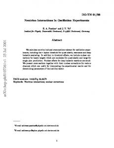
Figures 6 and 7 show the allowed regions in the sin2 2ϑeµ –∆m241 , sin2 2ϑee –∆m241 and sin2 2ϑµµ –∆m241 planes, respectively, together with the marginal ∆χ2 ’s for ∆m241 , sin2 2ϑeµ , sin2 2ϑee and sin2 2ϑµµ . The proposed NESSiE experiment aims at exploring these regions.

18

10 8

1

+

1

2 ∆m 41

[eV2]

0

2

4

∆χ2

6

3+1 68.27% C.L. (1σ) 90.00% C.L. 95.45% C.L. (2σ) 99.00% C.L. 99.73% C.L. (3σ)

10−1 10−4

10−3

10−2

10−1

si n 22ϑeµ

0

2

4

6

8

10

∆χ2

Figure 6: Allowed regions in the sin2 2ϑeµ –∆m241 plane and marginal ∆χ2 ’s for sin2 2ϑeµ and ∆m241 obtained from the global fit of all the considered data in 3+1 schemes. The best-fit point corresponding to χ2min is indicated by a cross. The isolated dark-blue dash-dotted contours enclose the regions allowed at 3σ by the analysis of appearance data (the ν¯µ → ν¯e data of the LSND, KARMEN and MiniBooNE experiments and the νµ → νe data of the NOMAD [26] and MiniBooNE experiments).

19

2 ∆m 41

[eV2]

0

2

4

∆χ2

6

8

10

1

1

+

+

10−1

10−1

10−1 10−3

10−2

1

si n 22ϑµµ

si n 22ϑee

Figure 7: Allowed regions in the sin2 2ϑee –∆m241 and sin2 2ϑµµ –∆m241 planes and marginal ∆χ2 ’s for sin2 2ϑee and sin2 2ϑµµ obtained from the global fit of all the considered data in 3+1 schemes. The best-fit point corresponding to χ2min is indicated by a cross. The line types and color have the same meaning as in Fig. 6. The isolated dark-blue dash-dotted lines are the 3σ exclusion curves obtained from reactor neutrino data in the left plot and from CDHS and atmospheric neutrino data in the right plot. The isolated dark-red long-dashed lines delimit the region allowed at 99% C.L. by the Gallium anomaly.

20

3.9

3+1 and CPT violation model

The only implementation among 3+1 models able to fit global data is the 3+1 and CPT violation model of Giunti-Laveder [3, 14]e . The model was inspired by the analysis of the electron neutrino data of the Gallium radioactive source experiments and the electron antineutrino data of the Bugey [22] and Chooz [23] reactor experiments in terms of neutrino oscillations allowing for a CPT-violating difference of the squared-masses and mixings of neutrinos and antineutrinos. It was found that the discrepancy between the disappearance of electron neutrinos indicated by the data of the Gallium radioactive source experiments and the limits on the disappearance of electron antineutrinos given by the data of reactor experiments reveal a positive CPT-violating asymmetry of the effective neutrino and antineutrino mixing angles. If there is a violation of the CPT symmetry, it is possible that the effective parameters governing neutrino and antineutrino oscillations are different. From a phenomenological point of view, it is interesting to consider the neutrino and antineutrino sectors independently, especially in view of the experimental tests considered in this proposal. The parameters of the model are reported in Tab. 6. ∆m241 1.92

|Ue4 | 0.275

2

|Uµ4 | ∆m41 0.0 0.47

|U e4 | 0.068

|U µ4 | 0.886

Table 6: Best fit parameters of the 3+1 and CPT violation model

In this scenario, neutrinos undergo νe → νe transitions only, see Fig. 8, while antineutrinos have a much richer phenomenology [28, 29]. The νe spectra computed for two years’ run at 30 kW are reported in Fig. 9. According to 3+1 and CPT violation model νe disappearance should be clearly detectable 1127 events detected against a prediction of 1424 for 0.3 < Eν < 2 GeV (Tab. 7). events ν mode ν mode ν mode

νe (0.3-2 GeV) νe (0.3-2 GeV) νµ (0.3-2 GeV)

No-Osc. 1424 1260 329328

Disapp. 1127 1254 277335

Disapp. + App. 1127 1699

Table 7: Events expectation for the 3+1 and CPT violation model

e

Indeed also“Non Standard Neutrino Interactions” or quantum decoherence have been proposed [27].

21

PHΝe®ΝeL

0.5

1.0 1.5 EΝ HGeVL

2.0

1.00 0.95 0.90 0.85 0.80 0.75 0.70 0.0

0.5

1.0 1.5 EΝ HGeVL

2.0

2.0

1.0 0.9 0.8 0.7 0.6 0.5 0.4 0.3 0.0

prob

0.90 0.85

1.0 1.5 EΝ HGeVL

0.80 0.0

2.0

0.5

1.0 1.5 EΝ HGeVL

2.0

PHΝ Μ®Ν ΜL

0.95

0.5

0.5

PHΝ e®Ν eL

1.00 prob

prob

PHΝ Μ®Ν eL

0.014 0.012 0.010 0.008 0.006 0.004 0.002 0.000 0.0

PHΝ Μ®Ν ΜL

1.0 0.8 0.6 0.4 0.2 0.0 0.0

prob

prob

prob

PHΝ Μ®ΝeL

0.014 0.012 0.010 0.008 0.006 0.004 0.002 0.000 0.0

1.0 1.5 EΝ HGeVL

0.5

1.0 1.5 EΝ HGeVL

2.0

Figure 8: Oscillation probabilities computed for the 3+1 and CPT violation model. P (νµ → νµ ) and P (νµ → νe ) are not displayed because they are predicted to be null by the model.

160 300

140

250 events

events

120 100 80 60

200 150 100 50

0.0

0.5

1.0

1.5

2.0

2.5

0 0.0 0.5 1.0 1.5 2.0 2.5 3.0 3.5 EΝ HGeVL

3.0

EΝ HGeVL 40 000 8000 6000 events

events

30 000 20 000 10 000 0 0.0

4000 2000 0

0.5

1.0

1.5

2.0

2.5

3.0

0.5

EΝ HGeVL

1.0

1.5

2.0

2.5

3.0

EΝ HGeVL

Figure 9: Top panel: νe event rates in the negative focussing beam (left) and ν e event rates in the positive focussing beam (right) computed assuming the 3+1 and CPT violation model. Non-oscillated rates are displayed as a blue histogram. Bottom panel: ν µ event rates in the positive focussing beam: on the right absolute event rates computed with (point with errors) and without (blue histogram) oscillations following the 3+1 and CPT violation model; on the left the difference between expected and measured events is shown.

22

4

The Neutrino Beam

The NESSiE detector is planned for exposure to the CERN-PS neutrino beam-line, originally used by the BEBC/PS180 collaboration [30] and re-considered later by the I216/P311 [31] proposal. The baseline setup used by BEBC/PS180 consisted in a 80 cm long, 6 mm diameter beryllium-oxide target followed by a single pulsed magnetic horn operated at 120 kA. The PS can deliver 3 · 1013 protons per cycle at 19.2 GeV kinetic energy in the form of 8 bunches of about 60 ns in a window of 2.1 µs, integrating about 1.25 · 1020 protons on target (p.o.t.)/year under reasonable assumptionsf . The existing decay tunnel, which has a cross section of 3.5 × 2.8 m2 for the first 25 m of length and 5.0 × 2.8 m2 for the remaining 20 m, is followed by a 4 m thick iron shield and 65 m of earth. With respect to the original configuration, the target and the horn must be redesigned and reconstructed due to the present level of radioactivity while the proton beam line magnets and supplies could be recovered (see Sect. 4.3).

4.1

Beam simulation

The BEBC/PS180 fluxes were reproduced by I216/P311 in their Letter of Intent [32] using a simulation based on GEANT3 and GFLUKA. The comparison was updated using a simulation adapted from the one used for the CNGS beam for their proposal [31]. For this memorandum a GEANT4 and FLUKA [33] based simulation has been developed to profit of a modern programming framework and to investigate possible improvements in the beam performance. The generation of proton-target interactions is done with FLUKA-2008 while GEANT4 is used for tracking in the magnetic field and the materials and for the treatment of meson decays. The simulation program, thoroughly described in [34], has been modified to take finite-distance effects into account, which are particularly important due to the short baselines involved (127 and 885 m measured from the target to the beginning of the LAr detector). Neutrinos crossing the LAr and Spectrometer volumes are directly scored using a full simulation avoiding any weighting approachg . A sample of 107 simulated p.o.t. was produced and has been used in the following. In order to benchmark the GEANT4 simulation the existing setup used for the BEBC/PS180 experiment has been reproduced [35]. The layout of the considered volumes is shown in Fig. 10. The spectrum shape of the νµ is in good agreement with that calculated by the I216/P311 experiment whereas the obtained normalization is instead 27% lower (Fig. 11). Investigations are ongoing to understand this difference, in particular the implementation of the geometry and the hadro-production models are under checking. f

180 days’ run per year allocating one third of the protons are assumed, with present performances. g This technique is relatively CPU-consuming but nevertheless affordable.

23

Figure 10: Layout of the focussing system and Near detector station in the GEANT4 simulation.

The flux reduction resulting from negative-focussing, which amounts to about 40%, is well reproduced. Neutrino fluxes at the Far and Near Spectrometers in positive and negativefocussing are shown in Fig. 12. Accounting for the Spectrometer geometries and locations we obtain a ratio ν/p.o.t. of about 10−2 in the Near station and a further reduction of a factor of about 20 in the Far location. The fractions of (νµ , ν¯µ , νe , ν¯e ) in the Near Spectrometer are (92.3, 6.6, 0.87, 0.26)% in positive-focussing mode and (12.2, 86.6, 0.49, 0.75)% in negative-focussing mode. In the Far detector numbers are very close to the previous ones. The electron neutrino contamination is in agreeement with the estimates of I216/P311. The energy dependence of the electron and wrong-sign muon contamination is shown in Fig. 13. It can be noticed that the νe contamination in the energy region between 500 M eV and 1 GeV is very low, approaching a minimum of 0.4%, to the benefit of the νe appearance search. The contamination of ν¯µ in the νµ beam is quite significant especially at high energy where the spectrometer charge separation becomes thus very important. In particular, after folding the spectrum with the CC cross section (Fig. 14), one can see that the negative-focussing beam at high energy yields a comparable mixture of µ− and µ+ . The Spectrometer charge separation allows studying the behavior of both CP states at the same time. The distribution of the impact points of the νµ in the Near Spectrometer is shown in the upper left plot of Fig. 15. The center of the beam is displaced in the bottom direction of 1 m and the radial beam profile can be well fitted with a Gaussian having a σ of about 4 m (Fig. 15 upper right and lower left plots) The spectrum of νµ at the Near detector peaks at lower energies due to the fact 24

POSITIVE FOCUSING

NEGATIVE FOCUSING

6

2

× 10

ν / 10 p.o.t. / GeV / m

BEBC/PS180 ν µ

90

I216/P311 ν µ

80 70

100

G4 x 1.27 ν µ

80

G4 ν µ

70

G4 ν µ

60

50

50

40

40

30

30

20

20

10

10

1 1.5

2

2.5

3

3.5

I216/P311 ν µ

90

60

0.5

× 10

13

G4 x 1.27 ν µ

13

ν / 10 p.o.t. / GeV / m

2

6

100

4 4.5 5 Eν (GeV)

0.5

1 1.5

2

2.5

3

3.5

4 4.5 5 Eν (GeV)

Figure 11: Comparison of the present simulation (dots) with those of BEBC (dashed line) and I216/P311 (continuous line) for positive-focussing mode (left) and negative-focussing mode (right). G4 stands for the new simulation obtained with GEANT4 which introduces a 1.27 reduction factor with respect to the old simulation. Fluxes are referred a distance of 825 m from the target (BEBC site). The target starts at 35 cm upstream of the BEBC/PS180 horn, which is operated at 120 kA.

6

ν / 10 p.o.t. / GeV / m 2

ν / 10 p.o.t. / GeV / m 2

× 10

3500

ν µ NEAR + foc.

3000 2500

ν µ NEAR + foc.

13

13

2000 1500 1000

6

ν µ FAR + foc.

50

ν µ FAR + foc.

40

30

20

10

500

0.5

1

1.5

2

2.5

3

3.5

4

4.5

5

0.5

Eν (GeV)

6

ν / 10 p.o.t. / GeV / m 2

× 10

ν / 10 p.o.t. / GeV / m 2

× 10 60

2500

ν µ NEAR - foc.

2000

ν µ NEAR - foc.

13

13

1500

1000

× 10

1

1.5

2

2.5

3

3.5

4

4.5

5

Eν (GeV)

6

40

ν µ FAR - foc.

35 30

ν µ FAR - foc.

25 20 15 10

500 5

0.5

1

1.5

2

2.5

3

3.5

4

4.5

5

0.5

Eν (GeV)

1

1.5

2

2.5

3

3.5

4

4.5

5

Eν (GeV)

Figure 12: νµ fluxes (black) and ν¯µ fluxes (red) at the Near (left column) and Far (right column) Spectrometers in positive-focussing (upper row) and negative-focussing (lower row) modes.

25

fraction

fraction

0.09

ν e/ ν µ + foc. 0.08

ν e/ ν µ - foc.

1

ν µ / ν µ + foc. ν µ / ν µ - foc.

0.8

0.07 0.06

0.6 0.05 0.04 0.4 0.03 0.02

0.2

0.01

0.5

1 1.5

2

2.5

3

3.5

4 4.5 5 Eν (GeV)

0.5

1 1.5

2

2.5

3

3.5

4 4.5 5 Eν (GeV)

Figure 13: Left: νe /νµ ratio in positive-focussing mode and ν¯e /¯ νµ ratio in negative-focussing mode in the Near Spectrometer as a function of the neutrino energy. Right: ν¯µ /νµ ratio in positivefocussing mode and νµ /¯ νµ ratio in negative-focussing mode in the Near Spectrometer as a function of the neutrino energy.

Event rates. M=0.6 ton, LAr, 2.5e20 pot, L=0.85 Km CC interactions

CC interactions

Event rates. M=0.6 ton, LAr, 2.5e20 pot, L=0.85 Km

νCC µ

50000

CC

νµ

40000

14000

νCC µ

12000

CC

νµ

10000 8000

30000

6000 20000 4000 10000 2000 0 0

0.5

1

1.5

2

2.5

3

3.5

4

0 0

4.5 5 Eν (GeV)

0.5

1

1.5

2

2.5

3

3.5

4

4.5 5 Eν (GeV)

Figure 14: Comparison of νµCC and ν¯µCC event rates for the positive (left) and negative-focussing (right) beams.

26

χ 2 / ndf Constant Mean_value Sigma

ν

y (m)

16

4

10000

14

3

8000

12 2

2.766 / 7 9679 ± 42.4 -0.167 ± 0.110 4.238 ± 0.219

10

6000

8

1

4000

6 0 4

2000

-1

-2

2

-4

-2

0

2

4

0

0 -2

x (m)

χ / ndf 15.28 / 15 Constant 6467 ± 29.5 Mean_value 0.0488 ± 0.0255 Sigma 4.01 ± 0.06

-1

0

1

2

3

4

y (m)

6000 5000

Eν (GeV)

ν

2

5 600

4.5 4

500

3.5 400

3

4000

2.5

300

3000 2

200

1.5

2000

1 100

1000 0.5 0

-4

-2

0

2

0 0

4

x (m)

1

2

3

4

5

0

radius (m)

Figure 15: Up left. Distribution of the neutrino impact points in the transverse plane, X vs Y . Up right: X projection. Bottom left: Y √ projection. The black histogram represents the νµ , the red histogram the ν¯µ . Bottom right: Eνµ vs X 2 + Y 2 . Results refer to positive-focussing mode.

that many interacting neutrinos are off-axis and then tend to have a lower mean energy (Fig 16, left). Nevertheless, restricting to the central region, i.e. the region that subtends an angle similar to that of the Far detector, the shapes tend to get closer. This selection allows smaller corrections in the Near/Far ratio thus decreasing the systematics. The correlation between the energy and the radius of the neutrino impact point is shown the lower right plot of Fig. 15. The shape of the νe spectrum on the other hand is more similar in the Near and Far locations (Fig 16, right) due to the predominantly 3-body decay origin.

4.2

New horn designs

By keeping the basic geometry of the beam (size of the target and horn hall, decay tunnel, shielding) unchanged, studies of several modified horns and targets in addition to the BEBC original setup are undergoing, an optimized design of new and possibly improved beam optics being pursued. Our aim is to move towards a high intensity νµ flux in order to reduce the statistical errors, peaking at hEνµ i ∼ 1 GeV to match the ∆m2 ∼ 1 eV2 region. For the reduction of systematics in the νµ → νe appearance channel the high energy tail above ∼ 2.5 GeV should be reduced to suppress π 0 production and the intrinsic νe contamination should be kept small. Preliminary studies performed with bi-parabolic horns `a la NuMI [36] indicate room for improvement. In particular in the last decades the feasibility of horns pulsed at high currents of order 300 kA has been demonstrated. The fluxes obtained with a 27

a.u.

a.u.

0.08

G4

!

FAR spectr.

0.25

G4 νe FAR LAr

0.07 0.2

G4

0.06

!

NEAR spectr.

G4 νe NEAR LAr 0.15

0.05 0.04

0.1 0.03 0.05

0.02 0.01 0

0 0.5

1

1.5

2

2.5

3

3.5

4

0.5

4.5 5 E (GeV)

1

1.5

2

2.5

3

3.5

4

4.5 5 Eν (GeV)

Figure 16: Comparison of the νµ (left) and νe (right) fluxes in the Near and Far LAr detector in positive-focussing mode. G4 stands for the new simulation obtained with GEANT4 which introduces a 1.27 reduction factor with respect to the old simulation.

new bi-parabolic horn pulsed at 246 kA, are shown in Fig. 17. An overall flux gain is obtained, particularly at low energy. This would be particularly useful to extend the sensitivity towards smaller ∆m2 . Since the interval of the interesting ∆m2 regions is large it would be desirable to get a configuration capable of scanning different neutrino energy regions thus adapting to the physics indications coming from the data taking. Despite the fact that the overall features of the neutrino beam are dictated by the proton energy, an effective way for varying the mean energy consists in using a tunable target-horn distance. While keeping the shape of the original horn unchanged, a scan in the scatter plane (current (i) vs target longitudinal position (ztarg )) was performed to study the effects of the fluxes in terms of νµ normalization, energy distribution and contaminations. Results are shown in Fig. 18 for positive-focussing at the Far location. Plots show how the integral νµ flux is increased going to higher currents; pushing the target upstream (downstream) corresponds to decrease (increase) the ν¯µ contamination and to probe the high(low)-energy region. Two configurations yielding very different spectra are shown in Fig. 19. It is interesting to notice that these fluxes are obtained using the same current of 300 kA just varying the position for the target.

4.3

Beam reactivation

Preliminary evaluations for a renovated TT7 PS neutrino beam line have been already completed at CERN [37]. The TT7 transfer line, the target chamber and the decay tunnel are in good shape and available for the installation of the proton beam line, target and magnetic horn. The main dipoles, quadrupoles, correction dipoles and possibly the transformer for the magnetic horn can be recuperated, reducing significantly the cost and time schedule. The target and secondary beam focussing design can profit of the CNGS experience as well as monitoring systems, primary

28

POSITIVE FOCUSING 2 "

G4 x 1.00

"

70

G4 x 1.00

"

"

100

I216/P311

90 80

G4

"

70

G4

"

60

60

50

50

40

40

30

30

20

20

10

10

1 1.5

2

2.5

3

3.5

! 10

"

13

80

I216/P311

/ 10 p.o.t. / GeV / m

BEBC/PS180

90

0.5

NEGATIVE FOCUSING

6

! 10

13

/ 10 p.o.t. / GeV / m

2

6

100

4 4.5 5 E (GeV)

0.5

1 1.5

2

2.5

3

3.5

4 4.5 5 E (GeV)

Figure 17: New horn fluxes compared to BEBC and I216/P311. The meaning of the symbols is as in Fig. 11, in particular G4 stands for the new simulation obtained with GEANT4 which introduces a 1.27 reduction factor with respect to the old simulation.

beam steering and target alignment [38]. The study dating back to 1999 [31] estimated the time required to be approximately 2 years for a total cost of about 4.2 MSF detailed as follows: • power converters of TT1 and TT7 magnets: consolidation and lower level electronics (1.1 MSF); • civil engineering, mostly new housing for converters (0.5 MSF); • removal of 400 m3 radioactive waste material in TT7, provisions and installations for radiation protections, access control (< 0.5 MSF); • beam line installation, vacuum chamber, general mechanics (0.4 MSF); • beam monitoring instrumentation (0.4 MSF); • new target and horn (0.4 MSF); • new pillars and platform in the Near experimental hall (50 KSF).

29

z target (m)

numu vs I vs Ztarg × 10

9

10000

0.3 0.2

8000

0.1 0

6000

-0.1 -0.2

4000 -0.3 -0.4

2000

-0.5 -0.6 100

150

200

250

300 current (kA)

0

1.6 0.3 1.4

0.2

(GeV)

z target (m)

vs I vs Ztarg

1.2

0.1 0

1

-0.1

0.8

-0.2 0.6

-0.3 -0.4

0.4

-0.5

0.2

-0.6 100

150

200

250

300 current (kA)

0

20

0.3

18 0.2 16

ν µ cont. (%)

z target (m)

anumu/numu (%) vs I vs Ztarg

0.1 14 0 12 -0.1

10

-0.2

8

-0.3

6

-0.4

4

-0.5

2

-0.6 100

150

200

250

300 current (kA)

0

Figure 18: Dependence of the integral νµ flux (top), the νµ mean energy (middle) and the ν¯µ contamination (bottom) from (I, ztarg ) with a test bi-parabolic horn. Results are shown for positivefocussing at the Far location.

30

× 10

6

80

ν µ/10

13

pot/m2/GeV

100

60

40

20

0

0.5

1

1.5

2

2.5

3

3.5

4

4.5 5 E(ν µ) (GeV)

Figure 19: Two extreme low (red) and high-energy (blue) configuration fluxes arising from the scan in the (I, ztarg ) plane. The current is 300 kA and the position of the beginning of the target with respect to the beginning of the horn is +32 and -58 cm respectively. The fluxes refer to a distance of 825 m.

31

5

Spectrometer Design Studies

The main purpose of a spectrometer placed downstream of the target section is to provide charge and momentum reconstruction of muons escaping from LAr detection. This choice would provide a double benefit with respect to a LAr detector running in stand-alone mode. Firstly a precise muon momentum reconstruction would allow a good kinematical closure of CC events occurred in LAr in particular in the high energy tail where the muon momentum resolution is poorer. Secondly muon charge separation would allow us to disentangle νµ and ν¯µ disappearance channels in particular in the negative-focussing option where wrong-sign contamination is larger. This would allow tackling CP and CPT violating scenarios in an unambiguous way. In addition, a proper mass-granularity combination would allow a coarse reconstruction of νµCC events occurring within the Spectrometer itself and provide a way to use the Spectrometer in stand-alone mode, too. We characterize the detector by evaluating the physics performances in terms of CC disappearance and the sensitiveness to (∆m2 , sin2 2θ) values predicted by the models described in Sect. 3. We recall that with a suitable detector the old CDHS νµ disappearance limit will be tested in just one day of data taking. Moreover we assumed some “a priori” constraints by defining a realistic, conservative, relatively inexpensive apparatus.

5.1

Magnetic field in Iron

A magnetized iron spectrometer was chosen as baseline option. Its design was such to match the required sensitivity of the experiment with respect to the sterile neutrino models of Sect. 3. The basic parameters to be tuned are the transverse widthh , the longitudinal dimensions, the iron slab thickness and the tracking detector resolution. The transverse and longitudinal dimensions constrain the detector acceptance and hence the detectable number of events which are directly related to the |Uµ4 | and |U µ4 | mixing parameters (see in particular Table 1 of Sect. 3). On the other hand the target segmentation sets bounds on muon momentum and charge reconstruction and 2 are directly related to ∆m241 and ∆m41 . The transverse width has to be large enough in order to maximize the detection of muons escaping from LAr. Monte Carlo simulation has shown that a transverse size matching the LAr acceptance (∼ 8 × 5 m2 in the Far site (FD) provides a good performance while still keeping the detector size at a feasible level (doubling the dimensions would improve the sensitivity to |Uµ4 | by 5%). Fig. 20 shows the muon impact point distribution along the x axis at FD. Due to the relatively low energy spectrum of the PS neutrino beam the Spectrometer longitudinal size has to be large enough in order to allow energy measureh

Here and in the following the transverse directions are defined by the horizontal x and the vertical y axis while the z axis runs in the beam direction.

32

200 180 160 140 120 100 80 60 40 20 0 -800

-600

-400

-200

0

200

400

600

800 x (cm)

Figure 20: Distribution of muon impact points along the x axis, at the Far site (FD). The dip at the center of the distribution and the sharp tails on the sides are due to the convolution with the LAr detector acceptance. The shaded area corresponds to the 78% of the total one.

33

Muon Momemtum Resolution

p/p

ment by range in a wide energy interval (see later on in this Section). Simulations have shown that 2 m of Iron contain ∼90% of muons in positive-focussing (∼85% in negative-focussing). 5 cm thick iron slabs would allow a spectrum bin size of ∼60÷100 √ MeV/ 12 ' 20 ÷ 30 MeV for perpendicularly impinging muons. Momentum reconstruction for passing-through muons (Eµ > 3 GeV/c) can be performed exploiting the track bending in the magnetic field. A detector resolution of ∼1 cm provides a σp /p resolution ranging from 20% at 3 GeV/c up to 30% at 10 GeV/c (see Fig. 21).

1 det

= 1.0 cm, ! = 5.0 cm and L = 1 m

MCS only, ! = 5.0 cm and L = 1 m

0.9

det det det

0.8

= 1.0 cm, ! = 5.0 cm and L = 2 m = 1.0 cm, ! = 2.5 cm and L = 1 m = 3.0 mm, ! = 5.0 cm and L = 1 m

Range measurement with ! = 5.0 cm and L = 1 m 10% charge misidentification level 1% charge misidentification level

0.7 0.6 0.5 0.4 0.3 0.2 0.1 0 10-1

2!10-1 3!10-1

1

2

3

4

5

6 7 8 9 10

20

Muon Momentum (GeV) Figure 21: Muon momentum resolution as calculated for several Spectrometer configurations, with a magnetic field B = 1.5 T .

Muon charge assignment is performed measuring the direction of track curvature. The experimental sensitivity to ∆m2 scales linearly with the neutrino energy, Eν , and √ only with 4 Nevents . Therefore the possibility to explore CPT-violating νµ disappearance at ∆m2 values below ∼1 eV2 in a baseline of ∼ 850 m relies on the capability to identify the muon charge with good accuracy down to Eν of about few hundreds of MeV and even lower if we consider the muon residual energy reaching the Spectrometer (see Fig. 22). However in this momentum region one has to cope with the severe limits imposed by Multiple Scattering in iron which completely dominates the charge identification capability. Since for stopping muons the path-length L in the B · L product is fixed by range B has to be as large as possible (B ' 1.5 T in iron). Once the magnetic field 34

Number of events 104

103

0

0.5

1

1.5

2

2.5

3

3.5 4 pµ (GeV/c)

Figure 22: Energy spectrum of µ+ intercepted by the Spectrometer in the FD in negative-focussing for 3.75 p.o.t. The shaded region is the subsample of muons from events such that 1.27 × 1 eV2 × L/Eν¯ > π/2.

35

is fixed the momentum resolution σp /p and the charge mis-identification η (defined as the fraction of muon tracks whose charge is wrongly assigned) are limited at low energies by Multiple Coulomb Scattering (MCS). In order to understand qualitatively this behavior let us define η as the fraction of muon tracks whose charge is wrongly assigned. η is related - in the Gaussian approximation of the Moliere distribution- to the momentum resolution by   1 1 η = erfc √ (9) 2 2(σp /p) where erfc is the complementary error function. The capability to separate chargeconjugated oscillation patterns depends on the available statistics and on the value of η: the lower the number of events the lower η has to be in order to assess a separation at a given significance level. For instance neglecting systematic and statistical uncertainties on η a ν/¯ ν separation at 10% level would require η ' 30% in energy bins with 10000 events and η ' 5% with 1000 events. The momentum resolution (or equivalently η) is the combination of two terms, the first one related to MCS and the other to measurement errors: s   2 2 σp σp σp = + (10) p p M CS p res The two terms can be calculated e.g. for the case of uniform detector spacing as in [39, 40, 41]. The first term is almost independent of the number of measurement points along the trajectory and it is expressed as 

σp p



 ' 27%

M CS

1.5T B



1m L

1/2 (11)

where L is the muon path-length in iron and is actually limited by the muon range and the spectrometer size at low and high momenta respectively. This term sets the lower irreducible limit that can be obtained by a measurement of this kind (note that η ' 5% roughly corresponds to σp /p ' 50%). The second term depends on the detector resolution and on the number of measurements (or equivalently on the iron slab thickness, ∆) and, in principle, can be decreased by changing the detector sampling and/or space resolution. In this case, for L >> 5∆, 

σp p



 ' 13%

res

p 1GeV/c



∆ 5cm

1/2 

1m L

5/2 

1.5T B



σdet  1cm

(12)

with the same considerations on L as for equation 11. Curves reported in Fig. 21 and Fig. 23 show the momentum resolution and the η dependence on the muon momentum for various choices of ∆ and σdet (for orthogonally 36

Muon Charge Misidentification

1

10-1

10-2

10-3

10-4

"det = 1.0 cm, ! = 5.0 cm and L = 1 m MCS only, ! = 5.0 cm and L = 1 m

10

-5

10

-6

"det = 1.0 cm, ! = 5.0 cm and L = 2 m "det = 1.0 cm, ! = 2.5 cm and L = 1 m

10-7 -1 10

"det = 5.0 mm, ! = 5.0 cm and L = 1 m

2!10-1 3!10-1

1

2

3

4

5

6 7 8 9 10

20

Muon Momentum (GeV) Figure 23: Muon charge mis-identification η as calculated for several Spectrometer configurations, with a magnetic field B = 1.5 T .

37

impinging muons). It is apparent that at best a mis-identification η below 5% can be obtained only for muons with momenta above ' 500 MeV/c. An option to improve charge identification capability below 500 MeV is to equip the Spectrometer with a magnetic field in air just in front of the first iron slab. This possibility is discussed in the next Section. From now on we will assume as baseline option for the FD site a dipolar magnetic Spectrometer made of two arms separated by 1 m air gap. Each arm consists of 21 iron slabs 585×875 cm2 wide and 5 cm thick interleaved with 2 cm gaps hosting 20 Resistive Plate Chambers (RPC) detectors with ∼1 cm tracking resolution. The Near detector (ND) Spectrometer is a downsized replica of the FD one, the only difference being in fact the transverse dimensions (351.5×625 cm2 ). A calculation of the magnetic field map was performed with the COMSOL code [42]. Fig. 24 shows the distribution of the magnetic field in the 21+21 iron layers (for convenience we show in the figure the entire magnetic system, i.e. in iron and in air, the latter to be discussed later on in the Section). The fringe field is 70 ÷ 100 G at 10 cm distance from the iron slab edge (Fig. 25). The simulation was performed assuming two symmetric coils wrapped around the top and bottom flux return path (following the same concept applied in the OPERA magnet [45]). The turns (36) are made of aluminum bars 27 × 19 mm2 with inner water cooling. The current density is 3 A/mm2 for a total current of 1255 A. The total resistance is 39 mOhm per coil, the voltage is 49 V and the power 61 kW . The conductor cross section can be increased to reduce the power dissipation.

5.2

Magnetic field in Air

For low momentum muons the effect of Multiple Scattering in iron is comparable to the magnetic bending and therefore the charge mis-identification increases (see Fig. 23) For muon momenta < 1 GeV /c the charge measurement can be performed by means of a magnetic field in air. In Fig. 26 the displacement expected in the bending plane is shown for muons crossing a magnetized air volume of 30 cm depth. A uniform magnetic field oriented along the y axis (the bending plane is the z, x one) is assumed. In the left plot the shift is shown as a function of the muon momentum for some values of the magnetic field in the 0.1 − 0.4 T range. In the right panel the spatial displacement in the bending plane estimated for muons of 0.5 GeV in a magnetic field of 0.3 T as a function of the incoming angles is plotted. A simulation of the magnetic field in air was realized based on a coil wound on a large conductor (54 mm × 19 mm) with 170 turns distributed along the spectrometer height. A uniform magnetic field of 0.25 T along the y axis is obtained with a coil current density of 8 A/mm2 (Fig. 24, 7000 A current). The fringe field at 10 cm distance from the edge (Fig 27) is 70 ÷ 200 G. The total resistance is 0.1 Ω, the voltage is 700 V and the power 4.9 M W . This set of parameters shall be intended as preliminary and needs to be optimized for reducing the electrical power and for 38

Figure 24: Simulated magnetic field distribution in the Iron Spectrometer (yellow regions) and in the air volume (light blue region on the left side, see Sect. 5.2). The horizontal axis is in meters; the color bar is in Tesla. The iron field is generated by two coils wrapped around the top and bottom iron flux return (only the upper coil is shown in the figure).

39

0/3

"#$%&'3(45'67")(8'-!!

9:;,&!&$'%(,!-

Figure 25: Magnetic field distribution in the 21+21 iron slabs and in the air volume upstream of the first iron slab. The vertical axis indicates the magnetic field in Tesla.

./2%?&;=> ./1%?&;=> ./0%?&;=> ./8%?&;=>

0

8/3

8

./3

9/ 1:1

9. 2/

1

2.

0: