Prostate Segmentation in 2D Ultrasound Images Using Image ...

Prostate Segmentation in 2D Ultrasound Images Using Image Warping and Ellipse Fitting Sara Badiei1 , Septimiu E. Salcudean1 , Jim Varah2 , and W. James Morris3 1

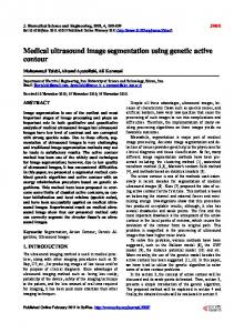
Department of Electrical and Computer Engineering, University of British Columbia, 2356 Main Mall, Vancouver, BC, V6T 1Z4, Canada {sarab, tims}@ece.ubc.ca 2 Department of Computer Science, University of British Columbia, Vancouver 3 Vancouver Cancer Center, British Columbia Cancer Agency, Vancouver

Abstract. This paper presents a new algorithm for the semi-automatic segmentation of the prostate from B-mode trans-rectal ultrasound (TRUS) images. The segmentation algorithm first uses image warping to make the prostate shape elliptical. Measurement points along the prostate boundary, obtained from an edge-detector, are then used to find the best elliptical fit to the warped prostate. The final segmentation result is obtained by applying a reverse warping algorithm to the elliptical fit. This algorithm was validated using manual segmentation by an expert observer on 17 midgland, pre-operative, TRUS images. Distancebased metrics between the manual and semi-automatic contours showed a mean absolute difference of 0.67 ± 0.18mm, which is significantly lower than inter-observer variability. Area-based metrics showed an average sensitivity greater than 97% and average accuracy greater than 93%. The proposed algorithm was almost two times faster than manual segmentation and has potential for real-time applications.

1

Introduction

Prostate cancer strikes one in every six men during their lifetime [1]. In recent years, increased prostate cancer awareness has led to an increase in the number of reported cases. As a result, prostate cancer research has increased dramatically, resulting in a 3.5% decrease in annual deaths due to this illness [1]. Interstitial brachytherapy is the most common curative treatment option for localized prostate cancer in North America. Improvements in ultrasound guidance technology, radioisotopes and planning software suggest an even greater increase in the number of brachytherapy procedures in the years to come [2]. In brachytherapy, small radioactive seeds are inserted into the prostate under TRUS guidance to irradiate and kill the prostate cells along with the tumor. Brachytherapy requires segmentation of the prostate boundary from TRUS images pre-operatively to generate the treatment plan, and post-operatively, to evaluate dose distribution and procedure success. Currently, oncologists segment the prostate boundary by hand. In this paper we emphasize the following requirements, used at the BC Cancer Agency, for prostate segmentation in 2D TRUS images: smooth, continuous R. Larsen, M. Nielsen, and J. Sporring (Eds.): MICCAI 2006, LNCS 4191, pp. 17–24, 2006. c Springer-Verlag Berlin Heidelberg 2006

18

S. Badiei et al.

contours with no sharp edges, no hourglass shapes and approximate symmetry about the median axis of the prostate. In pre and post-operative procedures, achieving these requirements manually is frustrating and time consuming. In intra-operative procedures, where prostate segmentation would enable real time updates to the treatment plan, manual prostate segmentation is unfeasible. It would be desirable to have an automatic or semi-automatic segmentation algorithm that satisfies the prostate segmentation criteria listed above but also has real time capabilities so that it can be incorporated into intra-operative procedures. A significant amount of effort has been dedicated to this area. Strictly edge-based algorithms such as [3, 4, 5, 6] result in poor segmentation due to speckle noise and poor contrast in TRUS images. One such edge-detection algorithm, introduced by Abolmaesumi et al. [6], uses a spatial Kalman filter along with Interacting Multiple Modes Probabilistic Data Association (IMMPDA) filters to detect the closed contour of the prostate. Although the IMMPDA edge-detector is capable of creating continuous contours, it cannot satisfy the smoothness and symmetry requirements on its own. In order to overcome these issues, deformable models such as those outlined in [7, 8, 9] were proposed. These techniques worked moderately well; however, the segmented shapes were not constrained and hourglass contours, for example, were possible. In order to constrain the prostate contours, groups such as Shen et al. [10] and Gong et al. [11] incorporated a priori knowledge of the possible prostate shapes into their algorithm. The automatic segmentation procedure of Shen et al. [10] combined a statistical shape model of the prostate, obtained from ten training samples, with rotation invariant Gabor features to initialize the prostate shape. This shape was then deformed in an adaptive, hierarchical manner until the technique converged to the final model. Unfortunately this technique is very expensive computationally, requiring over a minute to segment a single image. Gong et al. [11] modeled the prostate shape by fitting superellipses to 594 manually segmented prostate contours. These a priori prostate models, along with an edge map of the TRUS image, were then used in a Bayesian segmentation algorithm. The edge map was created by first applying a sticks filter, then an anisotropic diffusion filter and finally a global Canny edge-detector. In this technique, the pre-processing steps are computationally expensive and the global Canny edge-detector finds fragmented, discontinuous edges in the entire image. In this paper we have attempted to create an algorithm with low computational complexity that satisfies the smoothness and symmetry constraints and is driven by the clinical understanding of prostate brachytherapy. The proposed algorithm requires no computationally expensive pre-processing and is insensitive to the initialization points. The algorithm makes use of a novel image warping technique, ellipse fitting and locally applied IMMPDA edge-detection. The ellipse fitting procedure outlined in [12,13] solves a convex problem, is computationally cheap, robust and always returns an elliptical solution. The IMMPDA edge-detector is applied locally meaning that it finds continuous edges only along the boundary of the prostate instead of along the entire image. The method is described in more detail in the following section.

Prostate Segmentation in 2D Ultrasound Images

(a) Initialization

(b) Forward Warp

(c) First Ellipse Fit

(d) IMMPDA Edge Map

(e) Second Ellipse Fit

(f) Reverse Warp

19

Fig. 1. The proposed semi-automatic segmentation algorithm consists of six steps. Steps 1 and 2 show the unwarped (x-mark ) and warped (circles) initialization points respectively. Steps 3 and 5 show the best ellipse fit to the warped initialization points and to the IMMPDA edge map respectively. Step 6 shows the final segmentation result.

2

Segmentation Method

In the first step of our segmentation procedure the user selects six initialization points. Next, the image along with the initialization points are warped as outlined in Section 2.1. The warped prostate should look like an ellipse so that we can make use of the extensive literature on ellipse fitting to fit an initial ellipse to the six warped points as outlined in Section 2.2. This initial ellipse fit is used to confine and locally guide the IMMPDA edge-detector [6] along the boundary of the warped prostate to prevent the trajectory from wandering. A second ellipse is fit to the IMMPDA edge points, which provides a more accurate estimate of the warped prostate boundary. Finally, inverse warping is applied to the second elliptical fit to obtain the final segmented prostate contour. The only pre-processing required is a median filter (5x5 kernel) applied locally along the path of the edge-detector. The six step segmentation procedure outlined above is presented in Fig. 1. 2.1

Image Warping

The prostate is a walnut shaped organ with a roughly elliptical cross section. During image acquisition the TRUS probe is pressed anteriorly against the rectum wall which causes the 2D transverse image of the prostate to be deformed. A

S. Badiei et al.

Warping Function

20

1 0.8 0.6 0.4 4

0.2 0

3

100

2

80

theta (θ) 0−π

60

radius (r) 10−100

1

40 20 0

Fig. 2. The warping function: r /r = 1 − sin(θ) exp

−r 2 2σ 2

. The warped radius (r ) is

approximately equal to the unwarped radius (r) for angles (θ) close to 0 or π and for large r values. The warped radius (r ) is less than the unwarped radius (r) for angles (θ) close to π/2 and small r values; therefore, causing a stretch. The transition point between small and large r values is set by σ.

simple warping algorithm can be used to undo the effect caused by compression so that the prostate boundary in a 2D image looks like an ellipse. We assign a polar coordinate system to the TRUS image with origin on the TRUS probe axis, θ = 0 along the horizontal, and r ranging from Rmin to Rmax . We can undo the effect of the anterior compression caused by the TRUS probe by: i) stretching the image maximally around θ = π/2 and minimally around θ = 0 and θ = π, and ii) stretching the image maximally for small r values and minimally for large r values. These requirements suggest a sin(θ) dependence in the angular direction and a gaussian dependence in the radial direction. The resulting warping function is 2 −r . (1) r = r − r sin(θ) exp 2σ 2 where r represents the new warped radius, r is the unwarped radius, θ ranges from 0 to π and σ is a user selected variable that represents the amount of stretch in the radial direction (Fig. 2). Small σ values indicate less radial stretch and can be used for prostate shapes that are already elliptical and/or have experienced little deformation. Larger σ values indicate greater radial stretch and can be used for prostate shapes that have experienced more deformation by the TRUS probe. The advantages of this warping algorithm are that it is simple and intuitive with only one parameter to adjust. Due to time limits the σ was chosen separately for each image by trial and error. In the future we will automate the selection of σ. This and other more complex warping functions are being investigated as outlined in Section 5. 2.2

Ellipse Fitting

A general conic in 2D has the form F (X, P ) = X · P = P1 x2 + P2 xy + P3 y 2 + P4 x + P5 y + P6 = 0.

(2)


21

T where X = x2 xy y 2 x y 1 and P = P1 P2 P3 P4 P5 P6 . Given a set of points xi ,yi (i = 1 : n) around the boundary of a prostate in a 2D image, our goal is to find the best elliptical fit to these points. The problem reduces to finding the P vector that minimizes the following cost function subject to the constraint P T CP = 1 Cost =

n n (F (Xi , P ))2 = (Xi · P )2 = SP 2 . i=1

(3)

i=1

T T XnT , C is a 6x6 matrix of zeros with the upper Here S = X1T X2T ... Xn−1 left 3x3 matrix being [0 0 2; 0 -1 0; 2 0 0] and the P T CP = 1 constraint ensures elliptical fits only. The solution is the eigenvector P corresponding to the unique positive eigenvalue of the following generalized eigenvalue problem [12, 13]: (C − μS T S) = 0.

(4)

This ellipse fitting technique always returns a P vector that represents an ellipse regardless of the initial condition. Also, the fit has rotational and translational invariance, is robust, easy to implement and computationally cheap.

3

Experimental Results

Using the standard equipment (Siemens Sonoline Prima with 5MHz biplane TRUS probe) and the standard image acquisition procedure used at the BC Cancer Agency, we acquired 17 pre-operative TRUS images of the prostate from the midgland region. The images had low resolution and contained a superimposed needle grid. Although it is possible to obtain higher resolution images our goal was to work with the images currently used at the Cancer Agency. A single expert radiation oncologist with vast experience in prostate volume studies manually segmented the images using the Vari-Seed planning software from Varian. We then applied our semi-automatic segmentation algorithm and the same expert chose the initialization points. The algorithm was written in Matlab 7 (Release 14) and executed on a Pentium 4 PC running at 1.7 GHz. The image sizes were 480x640 with pixel size of 0.18 x 0.18mm. The times for manual and semi-automatic segmentation were recorded and are presented in Table 1. On average the time for manual segmentation, which includes the time for selecting 16-25 points and then re-adjusting them to obtain approximate symmetry, was 45.35 ± 4.85 seconds. The average time for semi-automatic segmentation, which includes the time to choose initialization points and then run the algorithm, was 25.35 ± 1.81 seconds. The average time to run the algorithm alone was 14.10 ± 0.20 seconds; however, we expect this time to decrease by at least five fold when the algorithm is transferred to C++. The manual segmentation was used as the ’gold standard’ while distance [14] and area [7] based metrics were used to validate the semi-automatic segmentation. For distance-based metrics we found the radial distance between the manual and semi-automatic contours, with respect to a reference point at the center of

22

S. Badiei et al. Table 1. Average times for manual and semi-automatic segmentation Manual Total time (sec) Mean STD 45.35 4.85

Semi-automatic (Matlab) Initialization (sec) Algorithm (sec) Total time (sec) Mean STD Mean STD Mean STD 11.26 1.81 14.10 0.20 25.35 1.81

Table 2. Average area and distance-based metrics for validation of segmentation algorithm Area-Based Metrics Sensitivity (%) Accuracy (%) Mean STD Mean STD 97.4 1.0 93.5 1.9

Distance-Based Metrics Sensitivity (mm) Accuracy (mm) Mean STD Mean STD 0.67 0.18 2.25 0.56

the prostate, as a function of theta around the prostate: rdif f (θ). The Mean Absolute Difference (MAD) and Maximum Difference (MAXD) were then found from rdif f (θ) as outlined in [14]. For area-based metrics we superimposed the manually segmented polygon, Ωm , on top of the semi-automatically segmented polygon, Ωa . The region common to both Ωm and Ωa is the True Positive (TP) area. The region common to Ωm but not Ωa is the False Negative (FN) area and the region common to Ωa but not Ωm is the False Positive (FP) area. We then found the following area-based metrics [7]: Sensitivity = T P/(T P + F N ).

(5)

Accuracy = 1 − (F P + F N )/(T P + F N ).

(6)

The MAD, MAXD, sensitivity and accuracy were found for each image and the overall average values along with standard deviations (std) are presented in Table 2. On average, the mean absolute difference between the manual and semi-automatic contours was 0.68 ± 0.18mm which is less than half the average variability between human experts (1.82 ± 1.44mm) [11]. Therefore, the mean absolute distance is on the same order of error as the repeatability between two different expert observers performing manual segmentation. On average, the maximum distance between the manual and semi-automatic contours was 2.25 ± 0.56mm. The average sensitivity and accuracy were over 97 and 93 percent respectively with std values less than 2%. Refer to Fig. 3 for sample outputs.

4

Discussion

The algorithm described above does not require training models or time consuming pre-filtering of TRUS images. The result is a simple, computationally inexpensive algorithm with potential for real-time applications and extension to 3D segmentation. Furthermore, the algorithm works well on the low resolution


23

Fig. 3. Comparison between manual segmentation (dotted line) and the proposed semiautomatic segmentation (solid line)

TRUS images currently used at the BC Cancer Agency and can be integrated easily into their setup without any changes to the image acquisition procedure. In preliminary studies, an untrained observer chose the initialization points. The segmented contour resulted in sensitivity and accuracy values over 90% with MAD and MAXD values less than 1 and 3mm respectively. This result shows that unlike most other semi-automatic segmentation techniques the success of the final segmentation does not rely on precise initialization of the prostate boundary. Consequently, during intra-operative procedures, a less experienced observer can choose the initialization points to update the treatment plan allowing the oncologist to continue their work uninterrupted. A more in-depth study of initialization sensitivity will be carried out in the future. Due to the nature of this technique, the algorithm works best for images that have an elliptical shape after warping and worst for images that have a diamond shape in the anterior region of the prostate.

5

Conclusion and Future Work

We have presented an algorithm for the semi-automatic segmentation of the prostate boundary from TRUS images. The algorithm is insensitive to the accuracy of the initialization points and makes use of image warping, ellipse fitting and the IMMPDA edge-detector to perform prostate segmentation. The merits of the algorithm lie in its straightforward, intuitive process but most importantly in its computational simplicity and ability to create good results despite non-ideal TRUS images.

24

S. Badiei et al.

There is significant potential for improving the warping function and we are currently working on two areas. First, we are attempting to implement an algorithm that will automatically choose the optimal σ and second, we would like to create a more complex warp function based on tissue strain information from elastography images [15]. It is our goal to extend this 2D semi-automatic segmentation algorithm to 3D in order to create real-time visualization tools for oncologists during pre, intra and post-operative procedures.

References 1. American Cancer Society: Key statistics about prostate cancer (2006) http://www. cancer.org. 2. Vicini, F., Kini, V., Edmundson, G., Gustafson, G., Stromberg, J., A., M.: A comprehensive review of prostate cancer brachytherapy: Defining an optimal technique. Int. J. Radiation Oncology Biol. Phys. 44 (1999) 483–491 3. Aarnink, R., Giesen, R., Huynen, A., de la Rosette, J., Debruyne, F., Wijkstra, H.: A practical clinical method for contour determination in ultrasonographic prostate images. Ultrasound Med. Biol. 20 (1994) 705–717 4. Pathak, S., Chalana, V., Haynor, D., Kim, Y.: Edge guided delineation of the prostate in transrectal ultrasound images. In: Proc. First Joint BMES/EMBS IEEE Conf. Volume 2. (1999) 1056 5. Kwoh, C., Teo, M., Ng, W., Tan, S., Jones, L.: Outlining the prostate boundary using the harmonics method. Med. Biol. Eng. Computing 36 (1998) 768–771 6. Abolmaesumi, P., Sirouspour, M.: An interacting multiple model probabilistic data association filter for cavity boundary extraction from ultrasound images. IEEE Trans. Med. Imaging 23 (2004) 772– 784 7. Ladak, H., Mao, F., Wang, Y., Downey, D., Steinman, D., Fenster, A.: Prostate boundary segmentation from 2d ultrasound images. Medical Physics 27 (2000) 1777–1788 8. Knoll, C., Alcaniz, M., Grau, V., Monserrat, C., Juan, M.: Outlining of the prostate using snakes with shape restrictions based on the wavelet transform. Pattern Recogn. 32 (1999) 1767–1781 9. Ghanei, A., Soltanian-Zadeh, H., Ratkewicz, A., Yin, F.: A three-dimensional deformable model for segmentation of human prostate from ultrasound images. Medical Physics 28 (2001) 2147–2153 10. Shen, D., Zhan, Y., Davatzikos, C.: Segmentation of prostate boundaries from ultrasound images using statistical shape model. IEEE Trans. Med. Imaging 22 (2003) 539– 551 11. Gong, L., Pathak, S., Haynor, D., Cho, P., Kim, Y.: Parametric shape modeling using deformable superellipses for prostate segmentation. IEEE Trans. Med. Imaging 23 (2004) 340– 349 12. Fitzgibbon, A., Pilu, M., Fisher, R.: Direct least square fitting of ellipses. IEEE Trans. Pattern Anal. Mach. Intellig. 21 (1999) 476–480 13. Varah, J.: Least squares data fitting with implicit function. BIT 36 (1996) 842–854 14. Chalana, V., Kim, Y.: A methodology for evaluation of boundary detection algorithms on medical images. IEEE Trans. Med. Imaging 16 (1997) 642–652 15. Turgay, E., Salcudean, S., Rohling, R.: Identifying mechanical properties of tissue by ultrasound. Ultrasound Med. Biol 32 (2006) 221–235