Protecting Moving Targets with Multiple Mobile Resources - Teamcore

P ROTECTING M OVING TARGETS WITH M ULTIPLE M OBILE R ESOURCES

Protecting Moving Targets with Multiple Mobile Resources Fei Fang Albert Xin Jiang Milind Tambe

FEIFANG @ USC . EDU JIANGX @ USC . EDU TAMBE @ USC . EDU

University of Southern California Los Angeles, CA 94035 USA

Abstract In recent years, Stackelberg Security Games have been successfully applied to solve resource allocation and scheduling problems in several security domains. However, previous work has mostly assumed that the targets are stationary relative to the defender and the attacker, leading to discrete game models with finite numbers of pure strategies. This paper in contrast focuses on protecting mobile targets that lead to a continuous set of strategies for the players. The problem is motivated by several real-world domains including protecting ferries with escort boats and protecting refugee supply lines. Our contributions include: (i) A new game model for multiple mobile defender resources and moving targets with a discretized strategy space for the defender and a continuous strategy space for the attacker. (ii) An efficient linear-programming-based solution that uses a compact representation for the defender’s mixed strategy, while accurately modeling the attacker’s continuous strategy using a novel sub-interval analysis method. (iii) Discussion and analysis of multiple heuristic methods for equilibrium refinement to improve robustness of defender’s mixed strategy. (iv) Discussion of approaches to sample actual defender schedules from the defender’s mixed strategy. (iv) Detailed experimental analysis of our algorithms in the ferry protection domain.1

1. Introduction In the last few years, game-theoretic decision support systems have been successfully deployed in several domains to assist security agencies (defenders) in protecting critical infrastructure such as ports, airports and air-transportation infrastructure (Tambe, 2011; Gatti, 2008; Marecki, Tesauro, & Segal, 2012; Jakob, Vanˇek, & Pˇechouˇcek, 2011). These decision support systems assist defenders in allocating and scheduling their limited resources to protect targets from adversaries. In particular, given limited security resources it is not possible to cover or secure all target at all times; and simultaneously, because the attacker can observe the defender’s daily schedules, any deterministic schedule by the defender can be exploited by the attacker (Paruchuri, Tambe, Ordonez, & Kraus, 2006; Kiekintveld, Islam, & Kreinovich, 2013; Vorobeychik & Singh, 2012; Conitzer & Sandholm, 2006). 1. A preliminary version of this work appears as the conference paper (Fang, Jiang, & Tambe, 2013). There are several major advances in this article: (i) Whereas the earlier work confined targets to move in 1-D space, we provide a significant extension of our algorithms (DASS and CASS) in this article to enable the targets and the patrollers to move in 2-D space; we also provide detailed experimental results on this 2-D extension. (ii) We provide additional novel equilibrium refinement approaches and experimentally compare their performance with the equilibrium refinement approach offered in our earlier work; this allows us to offer an improved understanding of the equilibrium refinement space. (iii) We discuss several sampling methods in detail to sample actual patrol routes from the mixed strategies we generate – a discussion that was missing in our earlier work. (iv) We provide detailed proofs that were omitted in the previous version of the work.

1

FANG , J IANG , & TAMBE

One game-theoretic model that has been deployed to schedule security resources in such domains is that of a Stackelberg game between a leader (the defender) and a follower (the attacker). In this model, the leader commits to a mixed strategy, which is a randomized schedule specified by a probability distribution over deterministic schedules; the follower then observes the distribution and plays a best response (Korzhyk, Conitzer, & Parr, 2010). Decision-support systems based on this model have been successfully deployed, including ARMOR at the LAX airport (Pita, Jain, Western, Portway, Tambe, Ordonez, Kraus, & Paruchuri, 2008), IRIS for the US Federal Air Marshals service (Tsai, Rathi, Kiekintveld, Ordón˜ ez, & Tambe, 2009), and PROTECT for the US Coast Guard (Shieh, An, Yang, Tambe, Baldwin, DiRenzo, Maule, & Meyer, 2012). Most previous work on game-theoretic models for security has assumed either stationary targets such as airport terminals (Pita et al., 2008), or targets that are stationary relative to the defender and the attacker, e.g., trains (Yin, Jiang, Johnson, Tambe, Kiekintveld, Leyton-Brown, Sandholm, & Sullivan, 2012) and planes (Tsai et al., 2009), where the players can only move along with the targets to protect or attack them). This stationary nature leads to discrete game models with finite numbers of pure strategies. In this paper we focus on security domains in which the defender needs to protect a mobile set of targets. The attacker can attack these targets at any point in time during their movement, leading to a continuous set of strategies. The defender can deploy a set of mobile escort resource(s) (called patrollers for short) to protect these targets. We assume the game is zero-sum, and allow the values of the targets to vary depending on their locations and time. The defender’s objective is to schedule the mobile escort resources to minimize attacker’s expected utility. We call this problem Multiple Mobile Resources protecting Moving Targets (MRMT). The first contribution of this paper is a novel game model for MRMT called MRMTsg . MRMTsg is an attacker-defender Stackelberg game model with a continuous set of strategies for the attacker. In contrast, while the defender’s strategy space is also continuous, we discretize it in MRMTsg for three reasons. Firstly, if we let the defender’s strategy space to be continuous, the space of mixed strategies for the defender would then have infinite dimensions, which makes exact computation infeasible. Secondly, in practice, the patrollers are not able to have such fine-grained control over their vehicles, which makes the actual defender’s strategy space effectively a discrete one. Finally, the discretized defender strategy is still valid in the original game with continuous strategy space for the defender, so the solution calculated under our formulation remains valid and gives a guarantee in terms of expected utility for the original continuous game. On the other hand, discretizing the attacker’s strategy space can be highly problematic as we will illustrate later in this paper. In particular, if we deploy a randomized schedule for the defender under the assumption that the attacker could only attack at certain descretized time points, the actual attacker could attack at some other time point, leading to a possibly worse outcome for the defender. Our second contribution is CASS (Solver for Continuous Attacker Strategies), an efficient linear program to exactly solve MRMTsg . Despite discretization, the defender strategy space still has an exponential number of pure strategies. We overcome this shortcoming by compactly representing the defender’s mixed strategies as marginal probability variables. On the attacker side, CASS exactly and efficiently models the attacker’s continuous strategy space using sub-interval analysis, which is based on the observation that given defender’s mixed strategy, the attacker’s expected utility is a piecewise-linear function. Along the way to presenting CASS, we present DASS (Solver for Discretized Attacker Strategies), which finds minimax solutions for MRMTsg games while constraining the attacker to attack at discretized time points. For clarity of exposition we first derive DASS and 2


CASS for the case where the targets move on a one-dimensional line segment. We later show that DASS and CASS can be extended to the case where targets move in a two-dimensional space. Our third contribution is focused on equilibrium refinement. Our game has multiple equilibria, and the defender strategy found by CASS can be suboptimal with respect to uncertainties in the attacker’s model, e.g., if the attacker can only attack during certain time intervals. We present two heuristic equilibrium refinement approaches for this game. The first, route-adjust, iteratively computes a defender strategy that dominates earlier strategies. The second, flow-adjust, is a linearprogramming-based approach. Our experiments show that flow-adjust is computationally faster than route-adjust but route-adjust is more effective in selecting robust equilibrium strategies. Additionally, we provide several sampling methods for generating practical patrol routes given the defender strategy in compact representation. Finally we present detailed experimental analyzes of our algorithm in the ferry protection domain. CASS has been deployed by the US Coast Guard since April 2013. The rest of the article is organized as follows: Section 2 will provide our problem statement. Section 3 will present the MRMTsg model and an initial formulation of the DASS and CASS for an one-dimensional setting. Section 4 will discuss equilibrium refinement, followed by Section 5 which will give the generalized formulation of DASS and CASS for two-dimensional setting. Section 6 will describe how to sample a patrol route and Section 7 will provide experimental results in the ferry protection domain. Section 8 will discuss related work. Section 9 concludes the article. At the end of the article, Appendix A provides a table listing all the notations used in the article.

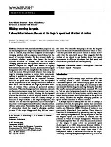
2. Problem Statement One major example of the practical domains motivating this paper is the problem of protecting ferries that carry passengers in many waterside cities. Packed with hundreds of passengers, these may present attractive targets to attack (e.g., with a small boat packed with explosives that may be only detected once it gets close to the ferry). Small, fast patrol boats can provide protection to such ferries (Figure 1(a)), but there are often limited numbers of patrol boats, i.e., they cannot protect the ferries at all times at all locations. We first focus on the case where ferries and patrol boats move in a one-dimensional line segment (this is a realistic setting and also simplifies exposition); we will discuss the two-dimensional case in Section 5. Domain description. In this problem, there are L moving targets, F1 , F2 , ..., FL . We assume that these targets move along a one-dimensional domain, specifically a straight line segment linking two terminal points which we will name A and B. This is sufficient to capture real-world domains such as ferries moving back-and-forth in a straight line between two terminals as they do in many ports around the world; an example is the green line shown in Figure 1(b). We will provide an illustration of our geometric formulation of the problem in Figure 2. The targets have fixed daily schedules. The schedule of each target can be described as a continuous function Sq : T → D where q = 1, ..., L is the index of the target, T = [0, 1] is a continuous time interval (e.g., representing the duration of a typical daily patrol shift) and D = [0, 1] is the continuous space of possible locations (normalized) with 0 corresponding to terminal A and 1 terminal B. Thus Sq (t) denotes the position of the target Fq at a specified time t. We assume Sq is piecewise linear. The defender has W mobile patrollers that can move along D to protect the targets, denoted as P1 , P2 , ..., PW . Although capable of moving faster than the targets, they have a maximum speed of vm . While the defender attempts to protect the targets, the attacker will choose a certain time and 3


(a)

(b)

Figure 1: (a) Protecting ferries with patrol boats; (b) Part of the map of New York Harbor Commuter Ferry Routes. The green straight line indicates a public ferry route run by New York City Department of Transportation.

a certain target to attack. (In the rest of the paper, we denote the defender as “she” and the attacker as “he”). The probability of attack success depends on the positions of the patrollers at that time. Specifically, each patroller can detect and try to intercept anything within the protection radius re but cannot detect the attacker prior to that radius. Thus, a patroller protects all targets within her protective circle of radius re (centered at her current position), as shown in Figure 2. ௘

ଶ

ଵ

ଶ

ଷ

ଵ

Figure 2: An example with three targets (triangles) and two patrollers (squares). The protective circles of the patrollers are shown with protection radius re . A patroller protects all targets in her protective circle. Patroller P1 is protecting F2 and P2 is protecting F3 . Symmetrically, a target is protected by all patrollers whose protective circles can cover it. If the attacker attacks a protected target, then the probability of successful attack is a decreasing function of the number of patrollers that are protecting the target. Formally, we use a set of coefficients {CG } to describe the strength of the protection. Definition 1. Let G ∈ {1, ..., W } be the total number of patrollers protecting a target Fq , i.e., there are G patrollers such that Fq is within radius re of each of the G patrollers. Then CG ∈ [0, 1] specifies the probability that the patrollers can successfully stop the attacker. We require that CG1 ≤ CG2 if G1 ≤ G2 , i.e., more patrollers offer better protection. As with previous work in security games (Tambe, 2011; Yin et al., 2012; Kiekintveld, Jain, Tsai, Pita, Ordonez, & Tambe, 2009), we model the game as a Stackelberg game, where the defender commits to a randomized strategy first, and then the attacker can respond to such a strategy. The 4


patrol schedules in these domains are currently created by hand; and hence suffer the drawbacks of hand-drawn patrols, including lack of randomness (in particular, informed randomness) and reliance on simple patrol patterns (Tambe, 2011), which we remedy in this paper. Defender strategy. A pure strategy of the defender is to designate a movement schedule for each patroller. Analogous to the target’s schedule, a patroller’s schedule can be written as a continuous function Ru : T → D where u = 1, ..., W is the index the patroller. Ru must be compatible with the patroller’s velocity range. Attacker strategy. The attacker conducts surveillance of the defender’s mixed strategy and the targets’ schedules; he may then execute a pure strategy response to attack a certain target at a certain time. The attacker’s pure strategy can be denoted as hq, ti where q is the index of target to attack and t is the time to attack. Utilities. We assume the game is zero-sum. If the attacker performs a successful attack on target Fq at location x at time t, he gets a positive reward Uq (x, t) and the defender gets −Uq (x, t), otherwise both players get utility zero. The positive reward Uq (x, t) is a known function which accounts for many factors in practice. For example, an attacker may be more effective in his attack when the target is stationary (such as at a terminal point) than when the target is in motion. As the target’s position is decided by the schedule, the utility function can be written as Uq (t) ≡ Uq (Sq (t), t). We assume that for each target Fq , Uq (t) can be represented as a piecewise linear function of t.

3. Models In this section, we introduce our MRMTsg model that uses a discretized strategy space for the defender and a continuous strategy space for the attacker. For clarity of exposition, we then introduce the DASS approach to compute a minimax solution for discretized attacker strategy space (Section 3.2), followed by CASS for the attacker’s continuous strategy space (Section 3.3). We first assume a single patroller in Sections 3.1 through 3.3 and then generalize to multiple patrollers in Section 3.4. Since our game is zero-sum, we use minimax (minimizing the maximum attacker utility) which returns the same solution as Strong Stackelberg Equilibrium (Fudenberg & Tirole, 1991; Korzhyk et al., 2010) for MRMTsg . 3.1 Representing Defender’s Strategies Since the defender’s strategy space is discretized, we assume that each patroller only makes changes at a finite set of time points T = {t1 , t2 , ..., tM }, evenly spaced across the original continuous time interval. t1 = 0 is the starting time and tM = 1 is the normalized ending time. We denote by δt the distance between two adjacent time points: δt = tk+1 − tk = M1−1 . We require δt to be small enough such that for each target Fq , the utility function Uq (t) and the moving schedule Sq (t) are linear within each interval [tk , tk+1 ] for k = 1, . . . , M − 1, i.e., the target is moving with uniform speed and linearly changing utility during each of these intervals. In addition to discretization in time, we also discretize the line segment AB that the targets move along into a set of points D = {d1 , d2 , ..., dN } and restrict each patroller to be located at one of the discretized points di at any discretized time point tk .2 During each time interval [tk , tk+1 ], each patroller moves with constant speed from her location di at time tk to her location dj at time 2. It is possible to have additional points where targets may stop (e.g., to load and unload passengers).

5


ĚŝƐƚĂŶĐĞ

tk+1 . The points d1 , d2 , ..., dN are ordered by their distance to terminal A, and d1 refers to A and dN refers to B. Since the time interval is discretized into M points, a patroller’s route Ru can be represented as a vector Ru = (dRu (1) , dRu (2) , ..., dRu (M ) ). Ru (k) is the index of the discretized distance point where the patroller is located at time tk . For expository purpose, we first focus on single defender resource and then generalize to larger number of resources later. For a single defender resource, the defender’s mixed strategy in full representation assigns a probability to each of the patrol routes that can be executed. Since at each time step a patroller can choose to go to at most N different locations, there are at most N M possible patrol routes in total and this number is achievable if there is no speed limit (or vm is large enough). The exponentially growing number of routes will make any analysis based on full representation intractable. Therefore, we use a compact representation of the defender’s mixed strategy where we represent the defender’s strategy with flow distribution variables {f (i, j, k)}. f (i, j, k) is the probability of the patroller moving from di at time tk to dj at time tk+1 . The complexity of the compact representation is O(M N 2 ), much more efficient compared to the full representation. Figure 3 shows a simple example illustrating the compact representation. Numbers on the edges indicate the value of f (i, j, k). We use Ei,j,k to denote the directed edge linking nodes (tk , di ) and (tk+1 , dj ). For example, f (2, 1, 1), the probability of the patroller moving from d2 to d1 during time t1 to t2 , is shown on the edge E2,1,1 from node (t1 , d2 ) to node (t2 , d1 ). While a similar compact representation was used earlier by Yin et al. (2012), we use it in a continuous setting.

݀ଶ ݀ଵ ‫ݐ‬ଵ

ƚŝŵĞ Ϭ͘ϲ ‫ݐ‬ ଶ

Ϭ͘ϲ

‫ݐ‬ଷ

Figure 3: Compact representation: x-axis shows time intervals; y-axis the discretized distancepoints in the one-dimensional movement space. Any strategy in full representation can be mapped into a compact representation. If there are H possible patrol routes R1 , R2 , ..., RH , a strategy in full representation can be denoted as a probability vector (p(R1 ), ...p(RH )) where p(Ru ) is the probability of taking route Ru . Taking route Ru means the patroller moves from dRu (k) to dRu (k+1) during time [tk , tk+1 ], so the edge ERu (k),Ru (k+1),k is taken when route Ru is chosen. Then the total probability of taking edge Ei,j,k is the sum of probabilities of all the routes Ru where Ru (k) = i and Ru (k + 1) = j. Formally, X f (i, j, k) = p(Ru ). (1) Ru :Ru (k)=i and Ru (k+1)=j

Different mixed strategies in full representation can be mapped to the same compact representation. Table 1 shows a simple example. Rows 1 and 2 show full representation for two mixed strategies. The probability of a route is labeled on all edges in the route in full representation. Adding up the numbers of a particular edge Ei,j,k in all routes of a full representation together, we can get f (i, j, k) for the compact representation (shown in Figure 3). 6


R1 = (d1 , d1 , d1 ) Ϭ͘ϲ

Ϭ͘ϲ

R1 = (d1 , d1 , d1 ) Ϭ͘Ϯ

Ϭ͘Ϯ

Full Representation 1 R2 = (d1 , d1 , d2 ) R3 = (d2 , d1 , d1 ) Ϭ

R4 = (d2 , d1 , d2 )

Ϭ

Full Representation 2 R2 = (d1 , d1 , d2 ) R3 = (d2 , d1 , d1 )

R4 = (d2 , d1 , d2 )

Ϭ͘ϰ

Ϭ͘ϰ

Table 1: Two full representations that can be mapped into the same compact representation shown in Figure 3.

This compact representation does not lead to any loss in solution quality. Recall our goal is to find an optimal defender strategy that minimizes maximum attacker expected utility. The attacker expected utility of attacking target Fq at time t given defender strategy f can be expressed as AttEUf (Fq , t) = (1 − C1 ω(Fq , t))Uq (t),

(2)

where Uq (t) is the reward for a successful attack, ω(Fq , t) is the probability that the patroller is protecting target Fq at time t and C1 is the protection coefficient of single patroller. We drop the subscript if f is obvious from the context. As C1 and Uq (t) are constants for a given attacker’s pure strategy hq, ti, AttEU(Fq , t) is purely decided by ω(Fq , t). As we will show in the next subsection, ω(Fq , t) can be calculated from the compact representation {f (i, j, k)}. If two defender strategies under the full representation are mapped to the same compact representation {f (i, j, k)}, they will have the same ω function and then they will have the same AttEU for any attacker’s pure strategy. We exploit the following properties of the compact representation. Property PN PN1. For any time interval [tk , tk+1 ], the sum of all flow distribution variables equals to 1: i=1 j=1 f (i, j, k) = 1. Property 2. The sum of flows that go into a particular node equals the sum PNof flows that go out of the node. Denote the sum for node (tk , di ) by p(i, k), then p(i, k) = j=1 f (j, i, k − 1) = PN j=1 f (i, j, k). Each p(i, k) is equal to the marginal probability that the patroller is at location di at time tk . P Property 3. Combining Property 1 and 2, N i=1 p(i, k) = 1. 3.2 DASS: Discretized Attacker Strategies DASS (Solver for Discretized Attacker Strategies) efficiently finds minimax solutions for MRMTsg based games under the assumption that the attacker will attack at one of the discretized time points tk . That is, we need to minimize v where v is the maximum of attacker’s expected utility. Here, v is the maximum of AttEU(Fq , t) for any target Fq at any discretized time point tk . From Equation (2), we know that AttEU(Fq , t) is decided by ω(Fq , t), the probability that the patroller is protecting target Fq at time t. Given the position of the target Sq (t), we define the 7


protection range βq (t) = [max{Sq (t) − re , d1 }, min{Sq (t) + re , dN }]. If the patroller is located within the range βq (t), the distance between the target and the patroller is no more than re and thus the patroller is protecting Fq at time t. So ω(Fq , t) is the probability that the patroller is located within range βq (t) at time t. For the discretized time points tk , the patroller can only be located at a discretized distance point di , so we define the following. Definition 2. I(i, q, k) is a function of two values. I(i, q, k) = 1 if di ∈ βq (tk ), and otherwise I(i, q, k) = 0. In other words, I(i, q, k) = 1 means that a patroller located at di at time tk is protecting target Fq . The probability that the patroller is at di at time tk is p(i, k). So we have ω(Fq , tk ) =

X i:I(i,q,k)=1

p(i, k),

X AttEU(Fq , tk ) = 1 − C1

i:I(i,q,k)=1

(3)

p(i, k) Uq (tk ).

(4)

Equation (4) follows from Equations (2) and (3), expressing attacker’s expected utility for discretized time points. Finally, we must address speed restrictions on the patroller. We set all flows corresponding to actions that are not achievable to zero,3 that is, f (i, j, k) = 0 if |dj − di | > vm δt. Thus, DASS can be formulated as a linear program. This linear program solves for any number of targets but only one defender resource. min

v

(5)

f (i,j,k),p(i,k)

f (i, j, k) ∈ [0, 1], ∀i, j, k

(6)

f (i, j, k) = 0, ∀i, j, k such that |dj − di | > vm δt

(7)

p(i, k) =

N X

f (j, i, k − 1), ∀i, ∀k > 1

(8)

f (i, j, k), ∀i, ∀k < M

(9)

j=1

p(i, k) =

N X j=1

N X

p(i, k) = 1, ∀k

(10)

i=1

v ≥ AttEU(Fq , tk ), ∀q, ∀k

(11)

Constraint 6 describes the probability range. Constraint 7 describes the speed limit. Constraints 8–9 describes Property 2. Constraint 10 is exactly Property 3. Property 1 can be derived from Property 2 and 3, so it is not listed as a constraint. Constraint (11) shows the attacker chooses the strategy that gives him the maximal expected utility among all possible attacks at discretized time points; where AttEU(·) is described by Equation (4). 3. Besides the speed limit, we can also model other practical restrictions of the domain by placing constraints on f (i, j, k).

8


3.3 CASS: Continuous Attacker Strategies Unfortunately, DASS’s solution quality guarantee may fail: if the attacker chooses to attack between tk and tk+1 , he may get a higher expected reward than attacking at tk or tk+1 . Consider the following example, with the defender’s compact strategy between tk and tk+1 shown in Figure 4. Here the defender’s strategy has only three non-zero flow variables f (3, 4, k) = 0.3, f (3, 1, k) = 0.2, and f (1, 3, k) = 0.5, indicated by the set of three edges E + = {E3,4,k , E3,1,k , E1,3,k }. A target Fq moves from d3 to d2 at constant speed during [tk , tk+1 ]. Its schedule is depicted by the straight line segment Sq . The dark lines L1q and L2q are parallel to Sq with distance re . The area between them indicates the protection range βq (t) for any time t ∈ (tk , tk+1 ). Consider the time points at which an r , r = 1 . . . 4 in Figure 4). Intuitively, edge from E + intersects one of L1q , L2q , and label them as θqk these are all the time points at which a defender patrol could potentially enter or leave the protection 0 and t 5 range of the target. To simplify the notation, we denote tk as θqk k+1 as θqk . For example, a 0 patroller moving from d3 to d4 (or equivalently, taking the edge E3,4,k ) protects the target from θqk 1 1 2 0 1 to θqk because E3,4,k is between L1 and L1 in [θqk , θqk ], during which the distance to the target is r and θ r+1 , for less or equal than protection radius re . Consider the sub-intervals between each θqk qk r = 0 . . . 4. Since within each of these five sub-intervals, no patroller enters or leaves the protection range, the probability that the target is being protected is a constant in each sub-interval, as shown in Figure 5(a).

ĚŝƐƚĂŶĐĞ

݀ସ ‫ݎ‬ ݀ଷ ‫ݎ‬௘ ௘ ݀ଶ ݀ଵ ଴ ଵ ଶ ଷ ସ ହ ߠ௤௞ ߠ௤௞ ߠ௤௞ ߠ௤௞ ߠ௤௞ ߠ௤௞ ‫ݐ‬௞ ‫ݐ‬௞ାଵ

ƚŝŵĞ

Figure 4: An example to show how a target moving from d3 to d2 during [tk , tk+1 ] is protected. In r , θ r+1 ], a patroller either always protects the target or never protects the a sub-interval [θqk qk target. Equivalently, the target is either always within the protective circle of a patroller or always outside the circle.

Suppose Uq (t) decreases linearly from 2 to 1 during [tk , tk+1 ] and C1 = 0.8. We can then calculate the attacker’s expected utility function AttEU(Fq , t) for (tk , tk+1 ), as plotted in Figure 5(b). AttEU(Fq , t) is linear in each sub-interval but the function is discontinuous at the intersection 1 , . . . , θ 4 because of the patroller leaving or entering the protection range of the target. points θqk qk 9


r from the left as: We denote the limit of AttEU when t approaches θqk r− lim AttEU(Fq , t) = AttEU(Fq , θqk )

r− t→θqk

Similarly, the right limit is denoted as: r+ lim AttEU(Fq , t) = AttEU(Fq , θqk )

r+ t→θqk

2 , getIf Fq is the only target, an attacker can choose to attack at a time immediately after θqk ting an expected utility that is arbitrarily close to 1.70. According to Equation (4), we can get 2+ AttEU(Fq , tk ) = 1.20 and AttEU(Fq , tk+1 ) = 1.00, both lower than AttEU(Fq , θqk ). Thus, the attacker can get a higher expected reward by attacking between tk and tk+1 , violating DASS’s quality guarantee.

0.50

1.70 1.43 1.20 1.00

0.20 0.00 ௞଴ ௞ଵ ௞ଶ ௞

௞ଷ

௞ସ

௞ହ ƚŝŵĞ ௞ାଵ

(a) Probability that the target is protected is a constant in each sub-interval.

௞଴ ௞ଵ ௞ଶ ௞

௞ଷ

௞ସ

௞ହ ƚŝŵĞ ௞ାଵ

(b) The attacker’s expected utility is linear in each sub-interval.

Figure 5: Sub-interval analysis in (tk , tk+1 ) for the example shown in Figure 4.] However, because of discontinuities in the attacker’s expected utility function, a maximum might not exist. This implies that the minimax solution concept might not be well-defined for our game. We thus define our solution concept to be minimizing the supremum of AttEU(Fq , t). Supremum is defined to be the smallest real number that is greater than or equal to any AttEU(Fq , t), i.e., it is the least upper bound. In the above example, the supremum of attacker’s expected utility 2+ in (tk , tk+1 ) is AttEU(Fq , θqk ) = 1.70. Formally, a defender strategy f is minimax if f ∈ arg minf 0 sup AttEUf 0 (Fq , t) How can we deal with the possible attacks between the discretized points and find an optimal defender strategy? We generalize the process above (called sub-interval analysis) to all possible edges Ei,j,k . We then make use of the piecewise linearity of AttEU(Fq , t) and the fact that the potential discontinuity points are fixed, which allows us to construct a linear program that solves the problem to optimality. We name the approach CASS (Solver for Continuous Attacker Strategies). We first introduce the general sub-interval analysis. For any target Fq and any time interval (tk , tk+1 ), we calculate the time points at which edges Ei,j,k and L1q , L2q intersect, denoted as interr ,r = 1...M , section points. We sort the intersection points in increasing order, denoted as θqk qk 10


M

0 = t and θ qk where Mqk is the total number of intersection points. Set θqk k qk r , θ r+1 ), r = 0, ..., M . (tk , tk+1 ) is divided into sub-intervals (θqk qk qk

+1

= tk+1 . Thus

Lemma 1. For any given target Fq , AttEU(Fq , t) is piecewise-linear in t. Furthermore, there exists a fixed set of time points, independent of the defender’s mixed strategy, such that AttEU(Fq , t) is r linear between each adjacent pair of points. Specifically, these points are the intersection points θqk defined above. r , θ r+1 ) for a target F , a feasible edge E Proof: In each sub-interval (θqk q i,j,k is either totally qk above or below L1q , and similarly for L2q . Otherwise there will be a new intersection point which contradicts the definition of the sub-intervals. If edge Ei,j,k is between L1q and L2q , the distance between a patroller taking the edge and target Fq is less than re , meaning the target is protected by the patroller. As edge Ei,j,k is taken with probability f (i, j, k), the total probability that the target is protected (ω(Fq , t)) is the sum of f (i, j, k) whose corresponding edge Ei,j,k is between the two lines in a sub-interval. So ω(Fq , t) is constant in t in each sub-interval and thus the attacker’s expected utility AttEU(Fq , t) is linear in each sub-interval according to Equation 2 as Uq (t) is linear in [tk , tk+1 ]. Discontinuity can only exist at these intersection points and an upper bound on the number of these points for target Fq is M N 2 . r , θ r+1 ), and Define coefficient Arqk (i, j) to be C1 if edge Ei,j,k is between L1q and L2q in (θqk qk 0 otherwise. According to Equation (2) and the fact that ω(Fq , t) is the sum of f (i, j, k) whose r , θ r+1 ). corresponding coefficient Arqk (i, j) = C1 , we have the following equation for t ∈ (θqk qk

 AttEU(Fq , t) = 1 −

N X N X

 Arqk (i, j)f (i, j, k) · Uq (t)

(12)

i=1 j=1

Piecewise linearity of AttEU(Fq , t) means the function is monotonic in each sub-interval and the supremum can be found at the intersection points. Because of linearity, the supremum of AttEU r , θ r+1 ) can only be chosen from the one-sided limits of the endpoints, AttEU(F , θ r+ ) and in (θqk q qk qk (r+1)−

AttEU(Fq , θqk

). Furthermore, if Uq (t) is decreasing in [tk , tk+1 ], the supremum is (r+1)− r+ AttEU(Fq , θqk ) and otherwise it is AttEU(Fq , θqk ). In other words, all other attacker’s strater+1 r r or θ r+1 . Thus, CASS adds new gies in (θqk , θqk ) are dominated by attacking at time close to θqk qk constraints to Constraints 6–11 which consider attacks to occur at t ∈ (tk , tk+1 ). We add one constraint for each sub-interval with respect to the possible supremum value in this sub-interval: min

v

(13)

f (i,j,k),p(i,k)

subject to constraints (6 . . . 11) (r+1)−

r+ v ≥ max{AttEU(Fq , θqk ), AttEU(Fq , θqk

)}

(14)

∀k ∈ {1 . . . M }, q ∈ {1 . . . L}, r ∈ {0 . . . Mqk } This linear program stands at the core of CASS and we will not differentiate the name for the solver and the name for the linear program in the following. All the linear constraints included by Constraint 14 can be added to CASS using Algorithm 1. The input of the algorithm include targets’ schedules {Sq }, the protection radius re , the speed limit vm , the set of discretized time points {tk } 11


and the set of discretized distance points {di }. Function CalInt(L1q , L2q , vm ) in Line 5 returns the list of all intersection time points between all possible edges Ei,j,k and the parallel lines L1q , L2q , with M

+1

qk r , θ r+1 ) in Line 7 0 and t . Function CalCoef(L1q , L2q , vm , θqk additional points tk as θqk k+1 as θqk qk returns the coefficient matrix Arqk . Arqk can be easily decided by checking the status at the midpoint r + θ r+1 )/2 and denote the patroller’s position at t in time. Set tmid = (θqk mid when edge Ei,j,k is qk taken as Ei,j,tmid , thus Arqk (i, j) = C1 if Ei,j,tmid ∈ βq (tmid ). Lines 8–11 add a constraint with

(r+1)−

r+ respect to the larger value of AttEU(Fq , θqk ) and AttEU(Fq , θqk ) to CASS for this sub-interval r+1 r (θqk , θqk ). It means when the attacker chooses to attack Fq in this sub-interval, his best choice is r , θ r+1 ). decided by the larger value of the two side-limits of AttEU in (θqk qk

Algorithm 1: Add constraints described in Constraint 14 1 2 3 4 5 6 7 8 9 10 11

Input: Sq , re , vm , {tk }, {di }; for k ← 1, . . . , M − 1 do for q ← 1, . . . , L do L1q ← Sq + re , L2q ← Sq − re ; M

+1

0 , . . . , θ qk ← CalInt(L1q , L2q , vm ); θqk qk for r ← 0, . . . , Mqk do r , θ r+1 ); Arqk ← CalCoef(L1q , L2q , vm , θqk qk if Uq (t) is decreasing in [tk , tk+1 ] then r+ ) add constraint v ≥ AttEU(Fq , θqk

else (r+1)− add constraint v ≥ AttEU(Fq , θqk )

Theorem 1. CASS computes (in polynomial time) the exact solution (minimax) of the game with discretized defender strategies and continuous attacker strategies. Proof: According to Lemma 1, AttEU(Fq , t) is piecewise linear and discontinuity can only ocr . These intersection points divide the time space into sub-intervals. cur at the intersection points θqk Because of piecewise linearity, the supremum of AttEU(Fq , t) equals to the limit of an endpoint of at least one sub-interval. For any defender’s strategy f that is feasible, a feasible v of the linear program 13-14 is no less than any of the limit values at the intersection points according to Constraint 14 and values at the discretized time points tk according to Constraint 11., and thus v can be any upper bound of AttEU(Fq , t) for f . As v is minimized in the objective function, v is no greater than the supremum of AttEU(Fq , t) given any defender strategy f , and further v will be the minimum of the set of supremum corresponding to all defender strategies. Thus we get the optimal defender strategy f , formally f = argf min sup AttEU(Fq , t) (15) The total number of variables in the linear program is O(M N 2 ). The number of constraints represented in Algorithm 1 is O(M N 2 L) as the number of intersection points is at most 2(M − 1)N 2 for each target. The number of constraints represented in Constraints 6–11 is O(M N 2 ). Thus, the linear program computes the solution in polynomial time. 12


Corollary 1. The solution of CASS provides a feasible defender strategy of the original continuous game and gives exact expected value of that strategy. 3.4 Generalized Model with Multiple Defender Resources When there are multiple patrollers, the patrollers will coordinate with each other. Recall the protection coefficient CG in Definition 1, a target is better protected when more patrollers are close to it (within radius re ). So the protection provided to a target is determined when all patrollers’ locations are known. Thus it is not sufficient to calculate the probability that an individual edge is taken as in the single patroller case. Under the presence of multiple patrollers, we need a more complex representation to explicitly describe the defender strategy. To illustrate generalization to the multiple defender resources case, we first take two patrollers as an example. If there are two patrollers, the patrol strategy can be represented using flow distribution variables {f (i1 , j1 , i2 , j2 , k)}. Here the flow distribution variables are defined on the Cartesian product of two duplicated sets of all feasible edges {Ei,j,k }. f (i1 , j1 , i2 , j2 , k) is the joint probability of the first patroller moving from di1 to dj1 and the second patroller moving from di2 to di2 during time tk to tk+1 , i.e., taking edge Ei1 ,j1 ,k and Ei2 ,j2 ,k respectively. The corresponding marginal distribution variable p(i1 , i2 , k) represents for the probability that the first patroller is at di1 and the second at di2 at time tk . Protection coefficients C1 and C2 are used when one or two patrollers are protecting the target respectively. So the attacker’s expected utility can be written as AttEU(Fq , t) = (1 − (C1 · ω1 (Fq , t) + C2 · ω2 (Fq , t))) · Uq (t) ω1 (Fq , t) is the probability that only one patroller is protecting the target Fq at time t and ω2 (Fq , t) is the probability that both patrollers are protecting the target. For attacks that happen at discretized points tk , we can make use of I(i, q, k) in Definition 2 and I(i1 , q, k)+I(i2 , q, k) is the total number of patrollers protecting the ferry at time tk . X ω1 (Fq , tk ) = p(i1 , i2 , k) i1 ,i2 :I(i1 ,q,k)+I(i2 ,q,k)=1 X ω2 (Fq , tk ) = p(i1 , i2 , k) i1 ,i2 :I(i1 ,q,k)+I(i2 ,q,k)=2

Constraints for attacks occurring in (tk , tk+1 ) can be calculated with an algorithm that looks the same as Algorithm 1. The main difference is in the coefficient matrix Arqk and the expression of AttEU. We set the values in the coefficient matrix Arqk (i1 , j1 , i2 , j2 ) as C2 if both edges Ei1 ,j1 ,k and Ei2 ,j2 ,k are between L1q and L2q , and C1 if only one of the edges protects the target. The attacker’s r , θ r+1 ) is expected utility function in (θqk qk X AttEU(Fq , t) = (1 − Arqk (i1 , j1 , i2 , j2 )f (i1 , j1 , i2 , j2 , k)) · Uq (t) i1 ,j1 ,i2 ,j2

For a general case of W defender resources, we can use {f (i1 , j1 , ..., iW , jW , k)} to represent the patrol strategy and get the following equations.   W X AttEU(Fq , t) = 1 − CQ · ωQ (Fq , t) · Uq (t) Q=1

ωQ (Fq , tk ) =

X i1 ,...,iW :

W P

p(i1 , . . . , iW , k) I(iu ,q,k)=Q

u=1

13


Q is the number of patrollers protecting the target, and is the probability of protection for the discretized time points tk . We can modify Algorithm 1 to apply for multiple defender resource case. Set Arqk (i1 , j1 , ..., iW , jW ) as CQ if Q of the edges {Eiu ,ju ,k } are between L1q and L2q . We conclude the linear program for generalized CASS for multiple patrollers as follows. min

v

(16)

f (i1 ,j1 ,...,iW ,jW ,k),p(i1 ,...,iW ,k)

f (i1 , j1 , . . . , iW , jW , k) = 0, ∀i1 , . . . , iW , j1 , . . . , jW such that ∃u, |dju − diu | > vm δt (17) p(i1 , . . . , iW , k) =

n X

...

n X

j1 =1

jW =1

n X

n X

f (j1 , i1 , . . . , jW , iW , k − 1), ∀i1 , . . . , iW , ∀k > 1 (18)

p(i1 , . . . , iW , k) =

...

j1 =1

f (i1 , j1 , . . . , iW , jW , k), ∀i1 , . . . , iW , ∀k < M

jW =1

(19) n X i1 =1

...

n X

p(i1 , . . . , iW , k) = 1, ∀k

(20)

iW =1


(21) (r+1)−


)}, ∀k, ∀q, ∀r

(22)

The number of variables in the linear program is O(M N 2W ) and the number of constraints is O(M N W ). While the expression grows exponentially in the number of resources, in real-world domains such as ferry protection, the number of defender resources are limited. That is the main reason that optimization using security games becomes critical. As a result, the above generalization of CASS is adequate at least for domains such as ferry protection. Further scale-up is an issue for future work.

4. Equilibrium Refinement A game often has multiple equilibria. Since our game is zero-sum, all equilibria achieve the same objective value. However, if an attacker deviates from his best response, some equilibrium strategies for the defender may provide better results than others. Consider the following example game. There are two targets moving during [t1 , t2 ] (no further discretization): one moves from d3 to d2 and the other moves from d1 to d2 (See Figure 6(a)). Suppose d3 − d2 = d2 − d1 = d and 5d/9 < re < d. There is only one patroller available and the protection coefficient C1 = 1. Both targets’ utility functions decrease from 10 to 1 in [t1 , t2 ] (See Figure 6(b)). In one equilibrium, f3,2,1 = f1,2,1 = 0.5, i.e., the patroller randomly chooses one target and follows it all the way. In another equilibrium, f3,3,1 = f1,1,1 = 0.5, i.e., the patroller either stays at d1 or at d3 . In either equilibrium, the attacker’s best response is to attack at t1 , with a maximum expected utility of 5. However, if an attacker is physically constrained (e.g., due to launch point locations) to only attack no earlier than t0 and t0 > θ11 (where θ11 is the intersection time point shown in Figure 6(a)), against both defender strategies he will choose to attack either of the targets at t0 . The attacker’s expected utility is Uq (t0 )/2 in the first equilibrium because there is 14


50% probability that the patroller is following that target. However in the second equilibrium, he is assured to succeed and get a utility of Uq (t0 ) because the distance between the chosen target and d1 (or d3 ) is larger than re at t0 , i.e., the chosen target is unprotected at t0 . In this case, the defender strategy in the first equilibrium is preferable to the one in the second; indeed, the first defender strategy (weakly) dominates the second one, by which we mean the first is no worse than the second no matter what strategy the attacker chooses. We provide a formal definition of dominance in Section 4.1.

ĚŝƐƚĂŶĐĞ

௤

݀ଷ

‫ݎ‬௘

10

‫ݎ‬௘

௤ ଴ 1

ܵଵ ݀ଶ ܵଶ

݀ଵ ‫ݐ‬ଵ

ߠଵଵ

‫ݐ‬଴

‫ݐ‬ଶ

ଵ

ƚŝŵĞ

ଵଵ

଴

ଶ

ƚŝŵĞ

(a) Two targets moves with schedules S1 and S2 . (b) Utility function is the same for both targets and is decreasing linearly over time.

Figure 6: An example to show one equilibrium outperforms another when the attacker is constrained to attack in [t0 , t2 ] if t0 > θ11 . Our goal is to improve the defender strategy so that it is more robust against constrained attackers while keeping the defender’s expected utility against unconstrained attackers the same. This task of selecting one from the multiple equilibria of a game is an instance of the equilibrium refinement problem, which has received extensive study in game theory (Fudenberg & Tirole, 1991; Miltersen & Sørensen, 2007). For finite security games, An, Tambe, Ordón˜ ez, Shieh, and Kiekintveld (2011) proposed techniques that provide refinement over Stackelberg equilibrium. However there has been little prior research on the computation of equilibrium refinements for continuous games. In this section, we introduce two equilibrium refinement approaches. Both approaches are based on the solution calculated by CASS. Recall that any strategy satisfying Constraints 16 – 22 can be a solution of CASS and one equilibrium is chosen depending on how the linear program solver is implemented. Assume we get an equilibrium (f 0 , hq 0 , t0 i) from CASS and now we attempt to select a more robust equilibrium based on it. The first approach, “route-adjust”, is a heuristic method that iteratively computes a defender strategy dominating f 0 . The second approach, “flow-adjust”, constructs M − 1 new linear programs based on f 0 to ensure the resulting defender strategy is robust when the attacker is constrained to attack in each time interval [tk , tk + 1]. For expository simplicity, we still use the single-resource case as an example, but both methods are applicable to the multiple-resources case. The results shown in evaluation section experimentally illustrates these two refinement methods can significantly improve the performance. 4.1 Route Adjust Given f is the defender strategy of one equilibrium of the game, if we can find a defender strategy f 0 such that for any attacker strategy (q, t), the defender’s expected utility under f 0 is equal to or higher 15


than the one under f , f 0 should be chosen for the defender as it is at least as good as the original strategy for any attacker strategy and may achieve better performance for some strategies. So an equilibrium with the dominant strategy f 0 is more robust to unknown deviations on the attacker side. We give the formal definition of dominance as follows. Definition 3. Defender strategy f dominates f 0 if DefEUf (Fq , t) ≥ DefEUf 0 (Fq , t), ∀q, t, or equivalently in this zero-sum game, AttEUf (Fq , t) ≤ AttEUf 0 (Fq , t). Corollary 2. Defender strategy f dominates f 0 if ∀q, t, ω(Fq , t) ≥ ω 0 (Fq , t). Corollary 2 follows from Equation (2). In this section, we introduce the route-adjust approach which gives a procedure for finding dominant strategy f 1 given the original strategy f 0 calculated by CASS. Route-adjust provides final routes using these steps: (i) decompose flow distribution f 0 into component routes; (ii) for each route, greedily find a route which provides better protection to targets; (iii) combine the resulting routes into a new flow distribution, f 1 , which dominates f 0 . To accomplish step (i), we decompose the flow distribution by iteratively finding a route that contains the edge with minimum probability. As shown in Figure 7, we first randomly choose a route that contains edge E1,2,2 , as f (1, 2, 2) = 0.4 is the minimum among all flow variables. We choose R2 = (d1 , d1 , d2 ), and set p(R2 ) = f (1, 2, 2) = 0.4. Then for each edge of the route R2 we subtract 0.4 from the original flow, resulting in a residual flow. We continue to extract routes from the residual flow until there is no route left. Denote by Z the number of non-zero edges in the flow distribution graph, then Z is decreased by at least 1 after each iteration. So the algorithm will terminate in at most Z steps and at most Z routes are found. The result of step (i) is a sparse description of a defender mixed strategy in full representation. As we will discuss in Section 6, this decomposition constitutes one method of executing a compact strategy. ଶ ଵ , ଵ , ଶ p R ଶ 0.4

ଵ ଵ , ଵ , ଵ p Rଵ 0.2

ଶ ଵ ଵ

ଶ ଵ ଵ

ଶ Ϭ͘ϰ ଶ

ଵ ଵ

ଷ

Ϭ͘ϲ

ଷ

ଵ ଵ

Ϭ͘Ϯ ଶ

ଷ

ଷ ଶ , ଵ , ଵ p R ଷ 0.4

ଶ Ϭ͘ϲ ଶ

Ϭ͘Ϯ

ଶ Ϭ͘Ϯ ଶ

Ϭ͘ϲ

ଷ

ଵ ଵ

Ϭ͘ϰ ଶ

ଷ

Figure 7: Step (i): decomposition. Every time a route containing the minimal flow variable is subtracted and a residual graph is left for further decomposition. The original flow distribution is thus decomposed into three routes R2 , R1 , and R3 with probability 0.4, 0.2 and 0.4 respectively.

16


For step (ii), we adjust each of the routes greedily. To that end, we first introduce the (weak) r and the coefficient matrix dominance relation of edges and routes, using the intersection points θqk Arqk (i, j) defined in Section 3.3. Definition 4. Edge Ei,j,k dominates edge Ei0 ,j 0 ,k in [tk , tk+1 ] if Arqk (i, j) ≥ Arqk (i0 , j 0 ), ∀q = 1..L, r , θ r+1 ] if edge E 0 0 protects it. Further, ∀r = 0..Mqk , i.e., edge Ei,j,k protects target Fq in [θqk i ,j ,k qk edge Ei,j,k strictly dominates edge Ei0 ,j 0 ,k if ∃q, r such that Arqk (i, j) > Arqk (i0 , j 0 ). The dominance relation of edges is based on the comparison of protection provided to the targets in each sub-interval. For example, in Figure 6(a), edge E1,2,1 dominate E1,1,1 as it always provide equal or better protection to both targets. Definition 5. Route Ru = (dRu (1) , . . . , dRu (M ) ) dominates Ru0 = (dRu0 (1) , . . . , dRu0 (M ) ) if ERu (k),Ru (k+1),k dominates edge ERu0 (k),Ru0 (k+1),k , ∀k = 1 . . . M − 1, i.e., route Ru dominates Ru0 if each edge of Ru dominates the corresponding edge in Ru0 . Denote the original route to be adjusted as Ru and the new route as Ru1 . A greedy way to improve the route is to replace only one node in the route. If we want to replace the node at time tk∗ , then we have Ru1 (k) = Ru (k), ∀k 6= k ∗ and dRu (k∗ ) in the original route is replaced with dRu1 (k∗ ) . So the patroller’s route changes only in [tk∗ −1 , tk∗ +1 ]. To simplify the notation, we denote the edge ERu (k∗ ),Ru (k∗ +1),k∗ as E(u, k ∗ ). Thus, only edges E(u, k ∗ − 1) and E(u, k ∗ ) in the original route are replaced by E(u1 , k ∗ − 1) and E(u1 , k ∗ ) in the new route. We want Ru1 to provide more protection to the targets, so the new route should dominate the original one. Therefore for a specified k ∗ , we are looking for a position dRu1 (k∗ ) such that: 1) E(u1 , k ∗ − 1) and E(u1 , k ∗ ) meet the speed constraint; 2) E(u1 , k ∗ − 1) and E(u1 , k ∗ ) dominates E(u, k ∗ − 1) and E(u, k ∗ ) respectively; 3) at least one of the edges E(u1 , k ∗ − 1) and E(u1 , k ∗ ) is not strictly dominated by the corresponding edges for any other choice of dRu1 (k∗ ) . The second requirement ensures the changed edges in the new route dominate the corresponding edges in the original route. Thus the new route Ru1 dominates Ru . The third requirement attains a local maxima. We can iterate this process for the new route and get a final route denoted by Ru0 after several iterations or when the state of convergence is reached. Note that we don’t require the new route to be different from the original route in each iteration. When the state of convergence is reached, the resulting route Ru0 keeps unchanged no matter which k ∗ is chosen for the next iteration. For the example in Figure 7, assume the only target’s moving schedule is d1 → d1 → d2 , d3 − d2 = d2 − d1 = δd, re = 0.1δd and utility function is constant. We adjust each route for only one iteration by changing the patroller’s position at time t3 , i.e., Ru (3). As t3 is the last discretized time point, only edge E(u, 2) may be changed. For R1 = (d1 , d1 , d1 ), we enumerate all possible patroller’s positions at time t3 and choose one according to the three constraints mentioned above. In this case, the candidates are d1 and d2 , so the corresponding new routes are R1 (unchanged) and R2 = (d1 , d1 , d2 ) respectively. Note that edge Ed1 ,d2 ,2 dominates Ed1 ,d1 ,2 because the former one protects the target all the way in [t2 , t3 ] and thus R2 dominates R1 . So d2 is chosen as the patroller’s position at t3 and R2 is chosen as the new route. The adjustment for all routes with non-zero probability after decomposition is shown in Table 2. The new routes we get after step (ii) dominate the original routes. That is, whenever a route Ru is chosen according to the defender mixed strategy resulting from step (i), it is always (weakly) better to instead take the corresponding new route Ru0 , because Ru0 provides more protection to the targets than Ru . Suppose there are H possible routes in the defender strategy after step (i), denoted as 17


Ru R1 = (d1 , d1 , d1 ) R2 = (d1 , d1 , d2 ) R3 = (d2 , d1 , d1 )

p(Ru ) after decomposition 0.2 0.4 0.4

Adjusted Routes (d1 , d1 , d2 ) = R2 (d1 , d1 , d2 ) = R2 (d2 , d1 , d2 ) = R4

Table 2: Step (ii): Adjust each route greedily.

R1 R2 R3 R4

Ru = (d1 , d1 , d1 ) = (d1 , d1 , d2 ) = (d2 , d1 , d1 ) = (d2 , d1 , d2 )

p0 (Ru ) after adjustment 0 0.6 0 0.4

Composed Flow Distribution ݀ଶ ݀ଵ ‫ݐ‬ଵ

Ϭ͘ϲ ‫ݐ‬ ଶ

‫ݐ‬ଷ

Table 3: Step (iii): compose a new compact representation. R1 , ..., RH . After adjusting the routes, we get a new defender strategy (p0 (R1 ), p0 (R2 ), ..., p0 (RH )) in full representation (See Table 3). Some routes are taken with higher probability (e.g. p0 (R2 ) = 0.2 + 0.4 = 0.6) and some are with lower probability (e.g. p0 (R3 ) = 0) compared to the original strategy. For step (iii), we reconstruct a new compact representation according to Equation 1. This is accomplished via a process that is the inverse of decomposition and is exactly the same as how we map a strategy in full representation into compact representation. For the example above, the result is shown in Table 3. Theorem 2. After steps (i)–(iii), we get a new defender strategy f 1 that dominates the original one f 0. Proof: We continue to use the notation that the decomposition in step (i) yields the routes R1 , ..., RH . For each flow distribution variable in the original distribution f 0 (i, j, k), it is decomposed into H sub-flows {fu0 (i, j, k)} according to the route decomposition. fu0 (i, j, k) = p(Ru ) if i = Ru (k), j = Ru (k + 1) and fu0 (i, j, k) = 0 otherwise. Thus we have the following equation. f 0 (i, j, k) = =

XH

f 0 (i, j, k) u=1 u

X u:Ru (k)=i,Ru (k+1)=j

(23) fu0 (i, j, k)

(24)

After adjust each route separately, each non-zero sub-flow fu0 (i, j, k) on edge E(u, k) is moved to edge E(u0 , k) as route Ru is adjusted to Ru0 . Reconstructing the flow distribution f 1 can also be regarded as adding up all the sub-flows after adjustment together on each edge. That means, f 1 is composed of a set of sub-flows after adjustment, denoted as {fu1 (i0 , j 0 , k)}. The subscript u represents for the index of the original route to indicate it is moved from edge E(u, k). So fu1 (i0 , j 0 , k) = fu0 (Ru (k), Ru (k + 1), k), if i0 = Ru0 (k) and j 0 = Ru0 (k + 1); otherwise fu1 (i0 , j 0 , k) = 0. Similarly to Equation 24, we have the following equation for f 1 . f 1 (i0 , j 0 , k) = =

XH

f 1 (i0 , j 0 , k) u=1 u

X u0 :Ru0 (k)=i0 ,Ru0 (k+1)=j 0

18

(25) fu1 (i0 , j 0 , k)

(26)


Based on how the adjustment is made, Ru0 dominates Ru and thus E(u0 , k) dominates E(u, k). So if edge E(u, k) protects target Fq at time t, the corresponding edge E(u0 , k) after adjustment also protects target Fq at time t. Recall from Section 3.3 that ω(Fq , t) is the sum of f (i, j, k) whose corresponding edge Ei,j,k can protect the target Fq at time t. We denote by ω 0 (Fq , t) and ω 1 (Fq , t) the probabilities of protection corresponding to f 0 and f 1 respectively. According to Equation 24, ω 0 (Fq , t) can be viewed as the sum of of all the non-zero sub-flows fu0 (i, j, k) where the corresponding E(u, k) protects the target Fq at time t. If fu0 (i, j, k) is a term in the summation to calculate ω 0 (Fq , t), it means E(u, k) protects Fq at t and thus the corresponding E(u0 , k) protects Fq at t, so the corresponding sub-flow fu1 (Ru0 (k), Ru0 (k + 1), k) in f 1 is also a term in the summation to calculate ω 1 (Fq , t). It leads to the conclusion ω 0 (Fq , t) ≤ ω 1 (Fq , t). According to Corollary 2, we have f 1 dominates f 0 . In the example in Figure 7, f 0 (1, 1, 2) is decomposed into two non-zero terms f10 (1, 1, 2) = 0.2 and f30 (1, 1, 2) = 0.4 along with routes R1 and R3 (See Figure 7). After adjustment, we get the corresponding subflows f11 (1, 2, 2) = 0.2, f31 (1, 2, 2) = 0.4. Recall that the target’s schedule is d1 → d1 → d2 . The flow distribution after adjustment (See Table 5) gives more protection to the target in [t2 , t3 ]. Since the flow is equal from t1 to t2 (and therefore the protection is the same), overall the new strategy dominates the old strategy. While step (iii) allows us to prove Theorem 2, notice that at the end of step (ii), we have a probability distribution over a set of routes from which we can sample actual patrol routes. For two or more defender resources, we define the dominance relation on the edge tuple (Ei1 ,j1 ,k , ..., EiW ,jW ,k ) with coefficient matrix for multiple patrollers Arqk (i1 , j1 , ..., iW , jW ). There are other ways to adjust each route. Instead of adjusting only one node in the route, we can adjust more consecutive nodes at a time, for example, we can adjust both Ru1 (k ∗ ) and Ru1 (k ∗ + 1) by checking edges E(u1 , k ∗ − 1), E(u1 , k ∗ ) and E(u1 , k ∗ + 1). However, we need to tradeoff the performance and the efficiency of the algorithm. This tradeoff will be further discussed in Section 7. 4.2 Flow Adjust Whereas route-adjust tries to select an equilibrium that is robust against attackers playing suboptimal strategies, the second approach, flow-adjust, attempts to select a new equilibrium that is robust to rational attackers that are constrained to attack during any time interval [tk , tk+1 ]. As we will discuss below, flow-adjust focuses on a weaker form of dominance, which implies that a larger set of strategies are now dominated (and thus could potentially be eliminated) compared to the standard notion of dominance used by route-adjust; however flow-adjust does not guarantee the elimination of all such dominated strategies. We denote by DefEUkf the defender expected utility when an attacker is constrained to attack during time interval [tk , tk+1 ] when the attacker provides his best response given the defender strategy f . Formally, DefEUkf = minq∈{1...L},t∈[tk ,tk+1 ] {DefEUf (Fq , t)}. We give the following definition of “local dominance”. Definition 6. Defender strategy f locally dominates f 0 if DefEUkf ≥ DefEUkf 0 , ∀k.4 Corollary 3. Defender strategy f locally dominates f 0 if min q∈{1...L},t∈[tk ,tk+1 ]

{DefEUf (Fq , t)} ≥

min q∈{1...L},t∈[tk ,tk+1 ]

4. We don’t require there exists at least one k such that DefEUkf > DefEUkf 0 .

19

{DefEUf 0 (Fq , t)}, ∀k,


or equivalently in this zero-sum game,

max q∈{1...L},t∈[tk ,tk+1 ]

{AttEUf (Fq , t)} ≤

max q∈{1...L},t∈[tk ,tk+1 ]

{AttEUf 0 (Fq , t)}, ∀k.

Corollary 3 follows from the fact that the attacker plays a best response given the defender strategy, and it means that f locally dominates f 0 if the maximum of attacker expected utilities in each time interval [tk , tk+1 ] given f is no greater than that of f 0 . Compared to Definition 3, which gives the standard condition for dominance, local dominance is a weaker condition; that is, if f dominates f 0 then f locally dominates f 0 , however the converse is not necessarily true. Intuitively, whereas in Definition 3 the attacker can play any (possibly suboptimal) strategy, here the attacker’s possible deviations from best response are more restricted. As a result, the set of locally-dominated strategies includes the set of dominated strategies. From Definition 6, if f locally dominates f 0 , and the attacker is rational (i.e., still playing a best response) but constrained to attack during some time interval [tk , tk+1 ], then f is preferable to f 0 for the defender. A further corollary is that even if the rational attacker is constrained to attack in the union of some of these intervals, f is still preferable to f 0 if f locally dominates f 0 . Also observe that the definition of local dominance depends on the time discretization. As we make finer and finer discretizations in the time dimension, i.e., as δt → 0, the attacker can choose from larger and larger sets of strategies, and the condition for local dominance approaches that of standard dominance. Flow-adjust looks for a defender strategy f 1 that locally dominates the original defender strategy To achieve this, we simply adjust the flow distribution variables f (i, j, k) while keeping the marginal probabilities p(i, k) the same. Figure 8 shows an example game with two discretized intervals [t1 , t2 ] and [t2 , t3 ] (only the first interval is shown). Suppose the maximal attacker expected utility is 5U0 in this equilibrium and is attained in the second interval [t2 , t3 ]. If the attacker’s utility for success is a constant U0 in the first interval [t1 , t2 ], then the defender strategy in [t1 , t2 ] could be arbitrarily chosen because the attacker’s expected utility in [t1 , t2 ] in worst case is smaller than that of the attacker’s best response in [t2 , t3 ]. However, if a attacker is constrained to attack in [t1 , t2 ] only, the defender strategy in the first interval will make a difference. In this example, there is only one target moving from d1 to d2 during [t1 , t2 ]. The schedule of the ferry is shown as dark lines and the parallel lines L11 and L21 with respect to protection radius re = 0.2(d2 − d1 ) are shown as dashed lines. The marginal distribution probabilities p(i, k) are all 0.5 and protection coefficient C1 = 1. In f 0 , the defender’s strategy is taking edges E1,1,1 and E2,2,1 with probability 0.5 and the attacker’s maximum expected utility is U0 , which can be achieved around time (t1 + t2 )/2 when neither of the two edges E1,1,1 and E2,2,1 are within the target’s protection range. If we adjust the flows to edge E1,2,1 and E2,1,1 , as shown in Figure 8(b), the attacker’s maximum expected utility in [t1 , t2 ] is reduced to 0.5U0 as edge E1,2,1 is within the target’s protection range all the way. So a rational attacker who is constrained to attack between [t1 , t2 ] will get a lower expected utility given defender strategy f 1 than given f 0 , and thus the equilibrium with f 1 is more robust to this kind of deviation on the attacker side. f 0.

So in flow-adjust, we construct M −1 new linear programs, one for each time interval [tk∗ , tk∗ +1 ], = 1 . . . M − 1 to find a new set of flow distribution probabilities f (i, j, k ∗ ) to achieve the lowest local maximum in [tk∗ , tk∗ +1 ] with unchanged p(i, k ∗ ) and p(i, k ∗ + 1). The linear program for an k∗

20


݀ଶ Ϭ͘ϱ

݀ଵ Ϭ͘ϱ ‫ݐ‬ଵ

Ϭ͘ϱ

Ϭ͘ϱ

Ϭ͘ϱ

݀ଶ Ϭ͘ϱ

Ϭ͘ϱ ‫ݐ‬ଶ

݀ଵ Ϭ͘ϱ ‫ݐ‬ଵ

(a) f 0 : the patroller is taking edges E1,1,1 and E2,2,1 with probability 0.5.

Ϭ

Ϭ͘ϱ

Ϭ͘ϱ ‫ݐ‬ଶ

Ϭ

(b) f 1 : the patroller is taking edges E1,2,1 and E2,1,1 with probability 0.5.

Figure 8: An example of flow adjust. An rational attacker who is constraint to attack in [t1 , t2 ] will choose to attack around time (t1 + t2 )/2 to get utility U0 given f 0 and attack around t1 or t2 to get utility 0.5U0 given f 1 . interval [t∗k , tk∗ +1 ] is shown below. min v

f (i,j,k∗ )

f (i, j, k ∗ ) = 0, if |dj − di | > vm ∗ δt n X p(i, k ∗ + 1) = f (j, i, k ∗ ), ∀i ∈ {1 . . . n} j=1

p(i, k ∗ ) =

n X

f (i, j, k ∗ ), ∀i ∈ {1 . . . n}

j=1

v ≥ AttEU (Fq , tk ), ∀q ∈ {1 . . . L}, k ∈ {k ∗ , k ∗ + 1} (r+1)−

r+ v ≥ max{AttEU (Fq , θqk ∗ ), AttEU (Fq , θqk ∗

)}

∀q ∈ {1 . . . L}, r ∈ {0 . . . Mqk∗ } While the above linear program appears similar to the linear program of CASS, they have significant differences. Unlike CASS, the marginal probabilities p(i, k ∗ ) here are known constants and are provided as input and as mentioned above, there is a seperate program for each [tk∗ , tk∗ +1 ]. Thus, we get f (i, j, k ∗ ) such that the local maximum in [tk∗ , tk∗ +1 ] is minimized. Denote the minimum as vk1∗ . From the original flow distribution f 0 , we get AttEUf 0 (Fq , t) and we denote the original local maximum value in [tk∗ , tk∗ +1 ] as vk0∗ . As the subset {f 0 (i, j, k ∗ )} of the original flow distribution f 0 is a feasible solution of the linear program above, we have vk1∗ ≤ vk0∗ , noting that the equality happens for the interval from which the attacker’s best response is chosen. Note that any change made to f (i, j, k) in an interval [t∗k , tk∗ +1 ] will not affect the performance of f in other intervals as the marginal probabilities p(i, k) are kept the same, i.e., changing f (i, j, k ∗ ) based on the linear program above is independent from any change to f (i, j, k), k 6= k ∗ . So we can solve the M − 1 linear programs independently. After calculating f (i, j, k ∗ ) for all k ∗ = 1..M − 1, we can get the new defender strategy f 1 by combining the solutions f (i, j, k ∗ ) of the different linear 21


programs together. As vk1∗ ≤ vk0∗ , we have max q∈{1...L},t∈[tk∗ ,tk∗ +1 ]

AttEUf 0 (Fq , t) ≤

max q∈{1...L},t∈[tk∗ ,tk∗ +1 ]

AttEUf 1 (Fq , t)

for all k ∗ = 1..M − 1, i.e., f 1 locally dominates f 0 . On the other hand, while we have restricted the strategies to have the same p(i, k), there may exist another strategy f 2 with a different set of p(i, k) that locally dominates f 1 . Finding locally dominating strategies with different p(i, k) from the original is a topic of future research.

5. Extension For Two-Dimensional Space Both DASS and CASS presented in Section 3 are based on the assumption that both the targets and the patrollers move along a straight line. However, a more complex model is needed in some practical domains. For example, Figure 9 shows a part of the route map of Washington State Ferries, where there are several ferry trajectories. If a number of patroller boats are tasked to protect all the ferries in this area, it is not necessarily optimal to simply assign a ferry trajectory to each of the patroller boat and calculate the patrolling strategies separately according to CASS described in Section 3. As the ferry trajectories are close to each other, a patrolling strategy that can take into account all the ferries in this area will be much more efficient, e.g., a patroller can protect a ferry moving from Seattle to Bremerton first, and then change direction halfway and protect another ferry moving from Bainbridge Island back to Seattle.

Figure 9: Part of route map of Washington State Ferries In this section, we extend the previous model to a more complex case, where the targets and patrollers move in a two-dimensional space and provide the corresponding linear-program-based solution. Again we use a single defender resource as an example, and generalize to multiple defenders at the end of this section. 5.1 Defender Strategy for 2-D As in the one-dimensional case, we need to discretize the time and space for the defender to calculate the defender’s optimal strategy. The time interval T is discretized into a set of time points T = {tk }. Let G = (V, E) represents the graph where the set of vertices V corresponds to the locations that the patrollers may be at, at the discretized time points in T , and E is the set of feasible edges that the patrollers can take. An edge e ∈ E satisfies the maximum speed limit of patroller and possibly other practical constraints (e.g., a small island may block some edges). 22


5.2 DASS for 2-D When the attack only occurs at the discretized time points, the linear program of DASS and described in Section 3 can be applied to the two-dimensional setting when the distance in Constraint 7 is substituted with Euclidean distance in 2-D space of nodes Vi and Vj . min

v

(27)

f (i,j,k),p(i,k)

f (i, j, k) ∈ [0, 1], ∀i, j, k

(28)

f (i, j, k) = 0, ∀i, j, k such that ||Vj − Vi || > vm δt

(29)

p(i, k) =

N X

f (j, i, k − 1), ∀i, ∀k > 1

(30)

f (i, j, k), ∀i, ∀k < M

(31)

j=1

p(i, k) =

N X j=1

N X

p(i, k) = 1, ∀k

(32)

i=1


(33)

Note that f (i, j, k) now represents the probability that a patroller is moving from node Vi to Vj during [tk , tk+1 ]. Recall in Figure 2, a patroller protects all targets within her protective circle of radius re . However, in the one-dimensional space, we only care about the straight line AB, so we used βq (t) = [max{Sq (t)−re , d1 }, min{Sq (t)+re , dN }] as the protection range of target Fq at time t, which is in essence a line segment. In contrast, here the whole circle needs to be considered as the protection range in the two-dimensional space and the extended protection range can be written as βq (t) = {V = (x, y) : ||V − Sq (t)|| ≤ re }. This change affects the value of I(i, q, k) and thus the value of AttEU (Fq , tk ) in Constraint 33. 5.3 CASS for 2-D When the attacking time t can be chosen from the continuous time interval T , we need to analyze the problem in a similar way as in Section 3.3. The protection radius is re , which means only patrollers located within the circle whose origin is Sq (t) and radius is re can protect target Fq . As we assume that the target will not change its speed and direction during time [tk , tk+1 ], the circle will also move along a line in the 2-D space. If we track the circle in a 3-D space where the x and y axes indicate the position in 2-D and the z axis is the time, we get an oblique cylinder, which is similar to a cylinder except that the top and bottom surfaces are displaced from each other (See Figure 5.3). When a patroller moves from vertex Vi (∈ V ) to vertex Vj during time [tk , tk+1 ], she protects the target only when she is within the surface. In the 3-D space we described above, the patroller’s movement can be represented as a straight line. Intuitively, there will be at most two intersection points between the patroller’s route in 3-D space and the surface. This can be proved by analytically calculating the exact time of these intersection points. Assume the patroller is moving from V1 = (x1 , y1 ) to V2 = (x2 , y2 ) and the target is moving from Sq (tk ) = (xˆ1 , yˆ1 ) to Sq (tk+1 ) = (xˆ2 , yˆ2 ) during [tk , tk+1 ] (an illustration is shown in Figure 5.3). The patroller’s position at a given time t ∈ [tk , tk+1 ] is denoted as (x, y) and the 23


dŝŵĞ ‫ݐ‬௞ାଵ

‫ݐ‬௔ ‫ݐ‬௞

Vଵ

Vଶ

ܵ௤ ሺ‫ݐ‬௞ାଵ ሻ

‫ݐ‬௕

ܵ௤ ሺ‫ݐ‬௞ ሻ

r௘

Figure 10: An illustration of the calculation of intersection points in the two-dimensional setting. The x and y axes indicates the position in 2-D and the z axis is the time. To simplify the illustration, z axis starts from time tk . In this example, there are two intersection points occurring at time points ta and tb .

target’s position is denoted as (ˆ x, yˆ). Then we have t − tk (y2 − y1 ) + y1 tk+1 − tk t − tk yˆ = (yˆ2 − yˆ1 ) + yˆ1 tk+1 − tk

t − tk (x2 − x1 ) + x1 , tk+1 − tk t − tk x ˆ= (xˆ2 − xˆ1 ) + x1 , tk+1 − tk

y=

x=

(34) (35)

At an intersection point, the distance from the patroller’s position to the target’s position equals to the protection radius re , so we are looking for a time t such that (x − x ˆ)2 + (y − yˆ)2 = re2

(36)

By substituting the variables in Equation 36 with Equations 34–35, and denoting (x2 − x1 ) − (xˆ2 − xˆ1 ) , tk+1 − tk (y2 − y1 ) − (yˆ2 − yˆ1 ) A2 = , tk+1 − tk A1 =

B1 = x1 − xˆ1 , B2 = y1 − yˆ1 ,

Equation 36 can be simplified to (A1 t − A1 tk + B1 )2 + (A2 t − A2 tk + B2 )2 = re2 .

(37)

Denote C1 = B1 − A1 tk and C2 = B2 − A2 tk , and we can easily get the two roots of this quadratic equation, which are p −2(A1 C1 + A2 C2 ) ± 2 (A1 C1 + A2 C2 )2 − (A21 + A22 )(C12 + C22 − re2 ) ta,b = . (38) 2(A21 + A22 ) 24


If a root is within the interval [tk , tk+1 ], it indicates that the patroller’s route intersects with the surface at this time point. So there will be at most two intersection points. Once we find all these intersection points, the same analysis in Section 3.3 applies and we can again claim Lemma 1. So we conclude that we only need to consider the attacker’s strategies at these intersection points. We r as in the one-dimensional case to denote the sorted intersection points and use the same notation θqk get the following linear program for the 2-D case. min

v

(39)

f (i,j,k),p(i,k)

subject to constraints(28 . . . 33) (r+1)−


)}

(40)

∀k ∈ {1 . . . M }, q ∈ {1 . . . L}, r ∈ {0 . . . Mqk } Algorithm 1 can still be used to add constraints to the linear program of CASS for the 2-D case. The main difference compared to CASS in the 1-D case is that since Euclidean distance in 2-D is used in Constraint 29 we need to use the extended definition of βq (t) in 2-D when deciding the entries in the coefficient matrix Arqk (i, j). For multiple defender resources, again the linear program described in Section 3.4 is applicable when the extended definition of βq (t) is used to calculate AttEU and Constraint 17 is substituted with the following constraint: f (i1 , j1 , . . . , iW , jW , k) = 0, ∀i1 , . . . , iW , j1 , . . . , jW such that ∃u, kVju − Viu k > vm δt.

6. Route Sampling We have discussed how to generate an optimal defender strategy in the compact representation; however, the defender strategy will be executed as taking a complete route. So we need to sample a complete route from the compact representation. In this section, we give two methods of sampling and show the corresponding defender strategy in the full representation when these methods are applied. The first method is to convert the strategy in the compact representation into a Markov strategy. A Markov strategy in our setting is a defender strategy such that the patroller’s movement from tk to tk+1 depends only on the location of the patroller at tk . We denote by α(i, j, k) the conditional probability of moving from di to dj during time tk to tk+1 given that the patroller is located at di at time tk . In other words α(i, j, k) represents the chance of taking edge Ei,j,k given that the patroller is already located at node (tk , di ). Thus, given a compact defender strategy specified by f (i, j, k) and p(i, k), we have α(i, j, k) = f (i, j, k)/p(i, k), if p(i, k) > 0. (41) α(i, j, k) can be an arbitrary number if p(i, k) = 0. We can get a sampled route by first determining where to start patrolling according to p(i, 1); then for each tk , randomly choose where to go from tk to tk+1 according to the conditional probability distribution α(i, j, k). The distribution from this sampling procedure matches the given marginal variables as each edge Ei,j,k is sampled with probability p(i, k)α(i, j, k) = f (i, j, k). This sampling method actually leads to a full representation where route Ru = (dRu (1) , dRu (2) , ..., dRu (M ) ) Q −1 is sampled with probability p(Ru (1), 1) M k=1 α(Ru (k), Ru (k + 1), k), the product of the probability of the initial distribution and the probability of taking each step. This method is intuitively 25


straightforward and the patrol route can be decided online during the patrol, i.e., the position of the patroller at tk+1 is decided when the patroller reaches its position at tk , which makes the defender strategy more unpredictable. The downside of the method is that the number of routes chosen with non-zero probability can be as high as N M . For 2-D case, the patroller is located at node Vi at time tk . The sampling process is exactly the same when α(i, j, k) is used to denote the probability of moving from Vi to Vj during [tk , tk+1 ]. The second method of sampling is based on the decomposition process mentioned in Section 4.1 (step (i)). As we discussed above for the first sampling method, sampling is essentially restoring a full representation from the compact representation. As shown in Table 1, there are multiple ways to assign probabilities to different routes and the decomposition process of “route-adjust” constructively defines one of them. So we can make use of the information we get from the process, and sample a route according to the probability assigned to each decomposed route. The number of routes chosen with non-zero probability is at most N 2 M , much less than the first method and thus it becomes feasible to describe the strategy in full representation, by only providing the routes that are chosen with positive probability.

7. Evaluation We use different settings in the ferry protection domain and compare the performance in terms of the attacker’s expected utility AttEU(Fq , t). As it is a zero-sum game, a lower value of AttEU indicates a higher value of defender’s expected utility. We will run experiments both for 1-D and 2-D setting. We will evaluate the performance of CASS and show the sampling results. We will also evaluate the improvement of the two refinement approaches for 1-D. Section 7.1 shows our results for the 1-D setting; Section 7.2 for the 2-D setting. 7.1 Experiments for One Dimensional Setting 7.1.1 E XPERIMENTAL S ETTINGS We used the following setting for the experiments in one dimensional case. This is a complex spatio-temporal game; rather than a discrete security game as in most previous work. There are three ferries moving between terminals A and B and the total distance AB = 1. The simulation time is 30 minutes. The schedules of the ferries are shown in Figure 11, where the x-axis indicates the time and the y-axis is the distance from terminal A. Ferry 1 and Ferry 3 are moving from A to B while Ferry 2 is moving from B to A. The maximum speed for patrollers is vm = 0.1/min and the protection radius is re = 0.1. Experiments in the one-dimensional case are using 2 patrollers (where C1 = 0.8, and C2 = 1.0), except in Section 7.1.5 where we report on experiments with different numbers of patrollers. 7.1.2 P ERFORMANCE OF S OLVERS We compare the strategies calculated by CASS with DASS and a baseline strategy. In the baseline strategy, the two patrollers choose a ferry with a probability of 1/3 (uniformly random) and move alongside it to offer it full protection, leaving the other two unprotected (strategy observed in practice). First we wished to stress-test CASS by using more complex utility functions than in the realistic case that follows. Therefore, we tested under 4 different discretization levels (details about discretization levels are included in Table 4) with random utilities, and at each discretization level, 26


d − distance

1

0.5

Ferry1 Ferry2 Ferry3

0 0

10

t − time

20

30

Figure 11: Schedules of the ferries we created 20 problem instances. In this ferry protection domain, the utility function for each ferry usually depends on the ferry’s position, so each instance has utilities uniformly randomly chosen between [0, 10] at discretized distance points; an example is shown in Figure 12(a). The chosen discretization levels have ensured that Uq (t) is linear in t in each time interval [tk , tk+1 ] for each target Fq . In Figure 12(a), the x-axis indicates the distance d from terminal A, the y-axis indicates the utility of a successful attack if the ferry is located at distance d. In Figure 12(b), x-axis plots the four discretization levels and y-axis plots the average attacker expected utility if he plays best response over the 20 instances for baseline, DASS and CASS. CASS is shown to outperform DASS and baseline (p < 0.01). e.g., at level 1, M = 4, N = 3, and at level 4, M = 16, and N = 11 Level 1 2 3 4

δt (minutes) 10 5 2.5 2

δd 0.5 0.25 0.125 0.1

M 4 7 13 16

N 3 5 9 11

Table 4: Details about discretization levels. In the experiments mentioned in this section, the distance space is evenly discretized, parameterized by δd = di+1 − di .

Next we turn to more realistic utility function in this ferry domain, which is of U -shape or inverse U -shape. Figure 13(a) shows a sample utility curve where the attacker gains higher utility closer to the shore. We fix the utility at the shore as 10, vary the utility in the middle (denoted as Umid ), which is the value on the floor of the U -shape or the top of the inverse U -shape and evaluate the strategies. In Figure 13(b), Umid is shown on x-axis and we compare performance of the strategies in terms of attacker’s expected utility when he plays best response on the y-axis. We conclude that 1) the strategy calculated by CASS outperforms the baseline and DASS; 2) DASS may actually achieve worse results than the baseline. Among all these different experiment settings of discretization and utility function, we choose one instance and provide a more detailed analysis for it. We refer to this instance as example setting in the following of this section. In this example setting, discretization level 4 is used and the utility curve is as shown in Figure 13(a), other parameters involved are described in Section 7.1.1. Figure 14 compares the attacker expected utility function when DASS and CASS is used respectively. The x-axis indicates the time t, and the y-axis indicates the attacker’s expected utility if he attacks Ferry 1 at time t. For the strategy calculated by DASS, the worst performance at discretized time points 27


Average Attacker EU

U − utility

10

5

0 0

0.5 d − distance

1

(a) Randomized attacker utility function

8 6

NAIVE DASS CASS

4 2 0

Level1 Level2 Level3 Level4

(b) Average solution quality of different strategies

Figure 12: Performance under different randomized utility function settings. The utility function in this set of experiments is a function of the distance to Terminal A. The utility function is piece-wise linear and the value at discretized distance points di is chosen randomly between [0,10].

15 Sup(AttEU)

U − utility

10 8 6 4 0

0.5 d − distance

10 5 0 0

1

(a) Realistic attacker utility function with Umid = 5

NAIVE DASS CASS

5

10 Umid

15

20

(b) Solution quality of different strategies

Figure 13: Performance under different realistic utility function settings. The utility function is U-shape or inverse U-shape. The utility around distance 0.5 is denoted as Umid . We compare the defender strategy given by DASS and CASS with the baseline when Umid is changing from 1 to 20.

is 3.50 (AttEU(F1 , 20)), however, the supremum of AttEU(F1 , t), t ∈ [0, 30] can be as high as 4.99 (AttEU(F1 , 4+ )), which experimentally shows that taking into consideration the attacks between the discretized time points is necessary. For the strategy calculated by CASS, the supremum of AttEU(F1 , t) is reduced to 3.82. 7.1.3 I MPROVEMENT U SING R EFINEMENT M ETHODS We compare the refinement approaches described in Section 4 and analyze the tradeoff between performance improvement and runtime. Three approaches are considered for comparison: routeadjust, flow-adjust and a variation of route-adjust, denoted by route-adjust2. In step (ii) of routeadjust, we replace every node in the route one-by-one in sequence.5 In step (ii) of route-adjust2, we replace every consecutive pair of nodes in the route in sequence. 5. In supplementary experiments, we also tested route-adjust with more iterations, e.g., repeating the process of replacing every node in sequence five times. The extra benefit is insignificant while the runtime increases proportionally to

28


5

AttEU

4 3 2

DASS CASS

1 0

10 20 t − time

30

4

4

3

3

AttEU

AttEU

Figure 14: The attacker’s expected utility function given the defender strategy calculated by DASS vs CASS under example setting. The expected utilities at the discretized time points are indicated by squares for CASS and dots for DASS. The maximum of AttEU under CASS is 3.82, 30%less than the maximum of AttEU under DASS, which is 4.99.

2 1 0

CASS Route−Adjust 10

t − time

20

2 1 0

30

(a) AttEU function of Ferry 1 after route-adjust (one node at a time)

Route−Adjust Route−Adjust2 10

t − time

20

30

(b) AttEU function of Ferry 1 after route-adjust2 (two nodes at a time)

AttEU

4 3 2 1 0

CASS Flow−Adjust 10

t − time

20

30

(c) Performance of flow-adjust

Figure 15: Performance of equilibrium refinement approaches. We first show results for the example setting. In Figure 15(a), we compare the AttEU(Fq , t) function of the defender strategy given by CASS and of the one after route-adjust for Ferry 1. It shows for an attack aiming at any target at any time, the defender strategy after route-adjust refinement is equally good or better than the one in the original equilibrium, and thus the defender performs equally or better no matter how the attacker is constrained in time, i.e., the defender stratethe number of iterations. In light of this, we choose to replace each node only once in the experiments reported in this article.

29


gy after route-adjust dominates the original strategy. Figure 15(b) is the comparison between AttEU function of the defender strategy after route-adjust and the one after route-adjust2 for Ferry 1. The one after route-adjust2 does not dominate the one after route-adjust but overall the former appears to perform better than the latter more frequently and by larger amounts. If we use the average value of AttEU function as a metric of performance, we will show that route-adjust2 is better than route-adjust in this example setting later in Table 5. Figure 15(c) shows the comparison between the AttEU function of the defender strategy given by CASS and that of the defender strategy after flow-adjust for Ferry 1. The strategy given by CASS is not dominated by the one after flow-adjust under Definition 3, but if we investigate the maximum of AttEU in each time interval [tk , tk+1 ], as shown in Table 6, we find that the defender strategy after flow-adjust locally dominates the original strategy. We list the worst case performance and the average performance of AttEU function over all ferries in this example setting for four defender strategies (CASS, route-adjust, route-adjust2, flowadjust) in Table 5, from which we conclude that 1) the worst case performance of all strategies of flow-adjust is the same, which means the defender achieves exactly same expected utility towards an unconstrained rational attacker; 2) the average performance of flow-adjust is slightly better than the CASS, but is outperformed by route-adjust and route-adjust2, while it takes much less time to run compared to the other two; 3) in this example setting, when we adjust two consecutive nodes at a time, the performance is better than adjusting only one node at a time, but the difference is not significant and it is much more expensive in terms of run-time. Strategies CASS Route-Adjust Route-Adjust2 Flow-Adjust

Worst Case Performance 3.82 3.82 3.82 3.82

Average Performance 3.40 2.88 2.76 3.34

Runtime (minutes) 8.96 32.31 0.50

Table 5: Comparison of different refinement approaches in terms of average performance and runtime. Only the runtime for the refinement process is calculated.

time interval [tk , tk+1 ] [2, 4] [4, 6] [6, 8] [8, 10] [10, 12] [12, 14] [14, 16]

maximum before refinement 3.7587 3.8182 3.8153 3.8137 3.8052 3.8050 3.7800

maximum after refinement

time interval [tk , tk+1 ]

3.6675 3.8182 3.6164 3.6316 3.6316 3.5664 3.2100

[16, 18] [18, 20] [20, 22] [22, 24] [24, 26] [26, 28] [28, 30]

maximum before refinement 3.8111 3.8182 3.8182 3.8182 3.8182 3.8182 3.8182

maximum after refinement 3.7291 3.8182 3.8182 3.8182 3.8182 3.8182 3.8182

Table 6: The maximum of attacker’s expected utility in each time interval decreases after flow adjustment

30


Figure 16(a) and Figure 16(b) shows the maximum and the average improvement of routeadjust, route-adjust2 and flow-adjust, averaged over all the 20 instances of Level 4 with randomized utilities that have been used for Figure 12(b); and Figure 16(c) shows the average runtime. The maximum improvement is the largest difference between the AttEU function given defender strategy calculated by CASS and the one after refinement. The average improvement is the average difference between the two functions. The standard deviations over all instances are shown as error bars. Figure 16 confirms that all the refinement approaches improve the defender strategy calculated by CASS in terms of both the maximum performance and average performance and thus provide better defender strategies given possible constrained attackers. Route-adjust2 achieves the most improvement, then route-adjust, and flow-adjust the least. Flow-adjust achieves much less improvement compared to the other two approaches and the difference between route-adjust2 and route-adjust is not as significant. In terms of run-time, flow-adjust is the least expensive, route-adjust the second and route-adjust2 the most. Route-adjust2 is significantly more expensive compared to the other two. So we conclude that route-adjust is a better choice considering the tradeoff between improvement and the runtime. 0.6

route−adjust route−adjust2 flow−adjust

2

Ave Improvement

Max Improvement

2.5

1.5 1 0.5 0

route−adjust route−adjust2 flow−adjust

0.4 0.2 0

Runtime (minutes)

(a) Average of maximal improvement

(b) Average of average improvement route−adjust route−adjust2 flow−adjust

40 30 20 10 0

(c) Average of runtime

Figure 16: Comparison of refinement approaches.

7.1.4 S AMPLED ROUTES We first convert the defender strategy under the example setting into a Markov strategy and sample 1000 pair of patrol routes. The defender strategy used here is the one after “route-adjust”. In each sample, a pair of routes is chosen step by step for the two patrol boats according to the joint conditional probability distribution {α(i1, j1, i2, j2, k)}. The routes for the two patrol routes are chosen simultaneously as they are coordinating with each other. We cannot show each pair seperately for all 1000 samples. Instead, Figure 17(a) shows the frequency of being taken out of the 1000 samples of each edge. The x-axis indicates the time and the y-axis is the distance to terminal A. The width 31


of the each edge indicates the frequency of being chosen by at least one patroller. Although Figure 17(a) does not precisely depict the samples, it provides a rough view of how the routes are taken by the patrol boats. Figure 17(b) shows the pair of routes that is of highest probability when we use the decomposition method of sampling. The solid lines show the patrol boats’ routes and the dashed lines show the ferries’ schedules. We get 3958 different pair of patrol routes in total in the decomposition process and the shown pair of routes is chosen with probability 1.57%. 1

d − distance

d − distance

1 0.8 0.6 0.4 0.2 0 0

5

10

15

20

25

0.8 0.6

0.2 0 0

30

t − time

Patrol Boat 1 Patrol Boat 2

0.4

5

10

15

20

25

30

t − time

(a)

(b)

Figure 17: Results for sampling under the example setting: (a) Frequency of each edge is chosen when the first sampling method based on Markov strategy is used. (b) Decomposed routes with highest probability superimposed on ferry schedules when the second sampling method based on decomposition is used.

7.1.5 N UMBER OF PATROLLERS Figure 18(a) shows the improvement in performance of CASS with increasing number of patrollers under discretization Level 1. The x-axis shows the number of patrollers and the y-axis indicates the average of attacker’s maximal expected utility, i.e., the expected reward when he plays his best response. The results are averaged over 20 random utility settings of discretization Level 1. With fewer patrollers, the performance of the defender varies a lot depending on the randomized utility function (as indicated by standard deviation shown as the error bar). But the variance gets much smaller with more patrollers, which means the defender has sufficient resources for different instances. Figure 18(b) shows the run-time for CASS; not surprisingly, the run-time increases when the number of patrollers increases. Figure 18(c) and 18(d) show the average performance and run-time of CASS with discretization Level 2, using the same set of utility settings as used in Level 1. Only results for 1 to 3 patrollers are shown. The program runs out of memory for 4 patrollers as there are N 8 M = 2734375 flow distribution variables and at least N 4 M = 8757 constraints. Note that the average solution quality of Level 2 is better than the result of Level 1 (e.g., the average attacker EU for 1 patroller is 4.81 in Level 1 and 4.13 in Level 2), which indicates a higher level of granularity can improve the solution quality. However, granularity clearly affect the ability to scale-up; which means that we need to consider the tradeoff between the solution quality and the memory used and one way to combat the scaling-up problem is to reduce the level of granularity. Nonetheless, the number of patrollers we have encountered in real-world scenarios such as at New York is of the order of 3 or 4, so CASS is capable at least for key real-world scenarios. 32


4

1 patroller 2 patrollers 3 patrollers 4 patrollers

Runtime (seconds)

Attacker EU

6

2 0

4 3 2 1 0

(a) Solution quality of Level 1

4

(b) Runtime of Level 1 40

1 patroller 2 patrollers 3 patrollers

Runtime (seconds)

Attacker EU

5

1 patroller 2 patrollers 3 patrollers 4 patrollers

3 2 1 0

30

1 patroller 2 patrollers 3 patrollers

20 10 0

(c) Solution quality of Level 2

(d) Runtime of Level 2

Figure 18: Performance with varying number of patrollers.

7.2 Experiments for Two Dimensional Setting The settings in 2-D space are more complex even with single patroller. Here we show an example setting motivated by the ferry system between Seattle, Bainbridge island and Bremerton as shown in Figure 9. In this example setting, three terminals (denoted as A,B and C) are non-collinear in the 2-D space as shown in the Figure 19(a). Ferry 1 and Ferry 2 are moving on the trajectory between Terminal B and C (denoted as Trajectory 1) and Ferry 3 and Ferry 4 are moving on the trajectory between Terminal B and A (denoted as Trajectory 2). The schedules of the four ferries are shown in Figure 19(b), where the x-axis is the time and the y-axis is the distance from the common terminal B. Ferry 1 moves from C to B, Ferry 2 moves from B to C, Ferry 3 moves from B to A and Ferry 4 moves from A to B. Similar to the one-dimensional scenario in ferry domain, we assume the utility is decided by the ferry’s position and the utility function is shown in Figure 19(c). The x-axis is the distance from the common terminal B and the y-axis is the utility for the two trajectories respectively. The 2-D space is discretized into a grid as shown in Figure 19(d) with δx = 1.5 and δy = 1 indicating the interval in the x-axis and y-axis. A patroller will be located at one of the intersection points of the grid graph at any discretized time points. The simulation time is 60 minutes and M = 13, i.e., tk+1 − tk = 5 minutes. The speed limit for the patroller is ve = 0.38 and all the available edges that a patroller can take during [tk , tk+1 ] are shown in Figure 19(d). Only one patroller is involved. The protection radius is set to re = 0.5, and protection coefficient is C1 = 0.8. Figure 20(a) compares the performance of DASS and CASS for Ferry 2. Ferry 2 is chosen because in both strategies, the attacker’s best response is to attack Ferry 2. The x-axis is the time t, and the y-axis is the attacker expected utility of attacking Ferry 1 at time t. The maximum of AttEU of CASS is 6.1466, 12% lower compared to the result of DASS, which is 6.9817. Figure 20(b) and 20(c) show two sampled route given the strategy calculated by CASS on the 2-D map 33


C

2

y

distance from Terminal B

Terminals in 2D Trajectory 1 B

1

Trajectory 2 0

A 0

1.5

3

4.5

x

Ferry Schedules 1

0.6 0.4 0.2 0 0

60

Edges Available 2

Ferry Trajectory1 Ferry Trajectory2

6

y

utility

40

(b) Ferry schedules

Utility Function 8

20

time

(a) Three terminals 10

Ferry1 Ferry2 Ferry3 Ferry4

0.8

1

4 2 0 0

0.2

0.4

0.6

0.8

0 0

1

1.5

3

4.5

x

distance from Terminal B (c) Utility function

(d) Available edges

Figure 19: An example setting in two-dimensional space where the dashed lines represents for the ferry trajectories. The patroller starts from the node with text “start” and follows the arrowed route, and ends at the node with text “end” at the end of the patrol. She may stay at the nodes with text “stay”. The patrol routes are shown in a intuitive way but can be ambiguous. The exact route should be listed as a table with time and position. The routes are sampled based on the converted Markov strategy, and the total number of patrol routes that may be chosen with non-zero probability is 4.49 × 1010 .

8. Related Work In this section we discuss literature related to our work. We will first discuss work on the computation of game-theoretic patrolling strategies, then discuss work on continuous games, and finally discuss work on equilibrium refinement. As mentioned in the introduction, Stackelberg games have been widely applied to security domains, although most of this work has considered static targets (e.g., Korzhyk et al., 2010; Krause, Roper, & Golovin, 2011; Letchford & Vorobeychik, 2012; Kiekintveld et al., 2013). Agmon, Kraus, and Kaminka (2008) proposed algorithms for computing mixed strategies for setting up a perimeter patrol in adversarial settings with mobile robot patrollers. Similarly, Basilico, Gatti, and Amigoni (2009) computed randomized leader strategies for robotic patrolling in environments with arbitrary topologies. Even when both of the players are mobile, e.g., in hider-seeker games (Halvorson, Conitzer, & Parr, 2009), infiltration games (Alpern, 1992) or search games (Gal, 1980), the targets (if any) were assumed to be static. Tsai et al. (2009) applied Stackelberg games to the domain of 34


Sampled Route by CASS

7

stay

6 y

AttEU

2

4 0

stay staystart end

1

DASS CASS

5

0

20 40 t − time

60

0

1.5

3

4.5

x

(a) Solution quality of DASSand CASS for Ferry (b) Sampled route 1 superimposed on ferry 2 trajectories

Sampled Route by CASS staystart

y

2

stay end

1

0 0

1.5

3

4.5

x (c) Sampled route 2 superimposed on ferry trajectories

Figure 20: Experimental results under two-dimensional setting

scheduling federal air marshals on board flights. The targets (i.e., flights) in this domain are mobile, but the players are restricted to move along the targets to protect or attack them. This stationary nature leads to discrete game models with finite numbers of pure strategies. Boˇsanský, Lisý, Jakob, and Pˇechouˇcek (2011) and Vanˇek, Jakob, Hrstka, and Pˇechouˇcek (2011) studied the problem of protecting moving targets. However, they both considered a model in which the defender, the attacker and targets have discretized movements on a directed graph. Such discretization of attacker strategy spaces can introduce suboptimality in the solutions, as we have shown with DASS. We, in our work, generalize the strategy space of the attacker to the continuous realm and compute optimal strategies even in such a setting. Furthermore, while we provide an efficient and scalable linear formulation, Boˇsanský et al. (2011) presented a formulation with non-linear constraints, which faced problems scaling up to larger games even with a single defender resource. Yin et al. (2012) considered the domain of patrolling in public transit networks (such as the LA Metro subway train system) in order to catch fare evaders. Because the players ride along trains that follow a fixed schedule, the domain is inherently discrete and they modeled the patrolling problem as a finite zero-sum Bayesian game. Yin et al. (2012) proposed a compact representation for defender mixed strategies as flows in a network. We adapt this compact representation idea to a continuous domain. In particular, in our domain we need to model the interaction between the 35


defender’s flow and attacker’s continuous strategy space. Our proposed sub-interval analysis used spatio-temporal reasoning to efficiently reduce the problem into a finite LP. Games with continuous strategy spaces have been well-studied in game theory. Much of the economics literature has focused on games whose equilibria can be solved analytically (and thus the question of computation does not arise), for example the classical theory of auctions (see e.g., Krishna, 2009). Recent computational approaches for the analysis and design of auctions have focused on discretized versions of the auction games (e.g., Thompson & Leyton-Brown, 2009; Daskalakis & Weinberg, 2012). There has been research on efficiently solving two-player continuous games with specific types of utility functions, such as zero-sum games with convex-concave utility functions (Owen, 1995) and separable continuous games with polynomial utility functions (Stein, Ozdaglar, & Parrilo, 2008). Johnson, Fang, and Tambe (2012) studied a continuous game model for protecting forests from illegal logging. In their model the target (i.e., the forest) is stationary, and with further simplifying assumptions (e.g., the forest having a circular shape) they were able to solve the game efficiently. In contrast to existing work, our game model has moving targets in a continuous domain, and the resulting utility functions are discontinuous and thus existing approaches are not applicable. Our CASS algorithm solves the game optimally without needing to discretize the attacker’s strategy space. There is an extensive literature on equilibrium refinement; however most existing work on the computation of equilibrium refinement focuses on finite games. For simultaneous-move finite games, solution concepts such as perfect equilibrium and proper equilibrium were proposed as refinements of Nash equilibrium (Fudenberg & Tirole, 1991). Miltersen and Sørensen (2007) proposed an efficient algorithm for computing proper equilibria in finite zero-sum games. For finite security games, An et al. (2011) proposed a refinement of Stackelberg equilibrium and techniques for computing such refinements. The resulting defender strategy is robust against possibilities of constrained capabilities of the attacker. These existing approaches rely on the finiteness of action sets, and is thus not applicable to our setting. Simon and Stinchcombe (1995) proposed definitions of perfect equilibrium and proper equilibrium for infinite games with continuous strategy sets, however they did not propose any computational procedure for the resulting solution concepts. Exact computation of equilibrium refinements of continuous games such as MRMTsg remains a challenging open problem.

9. Conclusion This paper makes several contributions in computing optimal strategies given moving targets and mobile patrollers. First, we introduce MRMTsg , a novel Stackelberg game model that takes into consideration spatial and temporal continuity. In this model, targets move with fixed schedules and the attacker chooses his attacking time from a continuous time interval. Multiple mobile defender recourses protect the targets within their protection radius, and bring in continuous space in our analysis. Second, we develop a fast solution approach, CASS, based on compact representation and sub-interval analysis. Compact representations dramatically reduce the number of variables in designing the optimal patrol strategy for the defender. Sub-interval analysis reveals the piece-wise linearity in attacker expected utility function and shows there is a finite set of dominating strategies for the attacker. Third, we propose two approaches for equilibrium refinement for CASS’s solutions: route-adjust and flow-adjust. Route-adjust decomposes the patrol routes, greedily improves the routes and composes the new routes together to get the new defender strategy. Flow-adjust is a fast 36


and simple algorithm that adjusts the flow distribution to achieve optimality in each time interval while keeping the marginal probability at the discretized time points unchanged. Additionally, we provide detailed experimental analysis in the ferry protection domain. CASS has been deployed by the US Coast Guard since April 2013. There are several important avenues for future work. These include: (i) use a decreasing function to model the protection provided to the targets instead of using a fixed protection radius; (ii) handle practical constraints on patrol boat schedule as not all are easily implementable; (iii) relax the constraints on schedules and utility functions.

10. Acknowledgements We thank the USCG officers, and particularly Craig Baldwin, Joe Direnzo and Francis Varrichio at sector New York, for their exceptional collaboration. This research is supported by US Coast Guard grant HSHQDC-10-D-00019 and MURI grant W911NF-11-1-0332.

37


Appendix A. Notation Table

Notation MRMT MRMTsg L Fq A, B T D Sq (t) W Pu vm re CG Uq (t) M N tk di δt Ru Ru (k) f (i, j, k) p(i, k) Ei,j,k p(Ru ) AttEU(Fq , t) βq (t) ω(Fq , t) I(i, q, k) L1q ,L2q r θqk r± AttEU(Fq , θqk ) Mqk Arqk (i, j) E(u, k)

Meaning The problem of multiple Mobile Resources protecting Moving Targets Game model with a continuous set of strategies for the attacker for MRMT. Number of ferries. Ferry with index q. Terminal points. Continuous time interval or a finite set of time points. Continuous space of possible locations or a set of distance points. Ferry schedule. Position of the target Fq at a specified time t. Number of patrollers. Patroller with index u. Speed limit of patroller. Protection radius of patroller. Probability that the attacker can be stopped with G patrollers. Positive reward of a successful attack on target Fq at time t for the attacker. Number of discretized time points. Number of discretized distance points. Discretized time point. Discretized distance point. Distance between two adjacent time points. Patrol route for patroller Pu . The patroller is located at dRu (k) at time tk . Flow distribution variable. Probability that the patroller moves from di to dj during time [tk , tk+1 ]. Marginal distribution variable. Probability that the patroller is located at di tk . The directed edge linking nodes (tk , di ) and (tk+1 , dj ). Probability of taking route Ru . Attacker expected utility of attacking target Fq at time t. Protection range of target Fq at time t Probability that the patroller is protecting target Fq at time t. Whether a patroller located at di at time tk is protecting target Fq . Lines of Sq (t) ± re . The rth intersection point in [tk , tk+1 ]. r . Left/right-side limit of AttEU(Fq , t) at θqk Number of intersection points in [tk , tk+1 ] with respect to target Fq . r , θ r+1 ; 0 otherwise. C1 if patroller taking edge Ei,j,k can protect target Fq in [θqk qk Short for ERu (k),Ru (k+1),k . Table 7: Summary of notations involved in the paper.

38


Bibliography Agmon, N., Kraus, S., & Kaminka, G. A. (2008). Multi-robot perimeter patrol in adversarial settings. In ICRA. Alpern, S. (1992). Infiltration Games on Arbitrary Graphs. Journal of Mathematical Analysis and Applications, 163, 286–288. An, B., Tambe, M., Ordón˜ ez, F., Shieh, E., & Kiekintveld, C. (2011). Refinement of strong stackelberg equilibria in security games. In AAAI. Basilico, N., Gatti, N., & Amigoni, F. (2009). Leader-follower strategies for robotic patrolling in environments with arbitrary topologies. In AAMAS. Boˇsanský, B., Lisý, V., Jakob, M., & Pˇechouˇcek, M. (2011). Computing time-dependent policies for patrolling games with mobile targets. In AAMAS. Conitzer, V., & Sandholm, T. (2006). Computing the optimal strategy to commit to. In EC. Daskalakis, C., & Weinberg, M. (2012). Symmetries and optimal multi-dimensional mechanism design. In ACM Conference on Electronic Commerce. Fang, F., Jiang, A. X., & Tambe, M. (2013). Optimal patrol strategy for protecting moving targets with multiple mobile resources. In International Conference on Autonomous Agents and Multiagent Systems (AAMAS). Fudenberg, D., & Tirole, J. (1991). Game Theory. MIT Press. Gal, S. (1980). Search Games. Academic Press, New York. Gatti, N. (2008). Game theoretical insights in strategic patrolling: Model and algorithm in normalform. In ECAI, pp. 403–407. Halvorson, E., Conitzer, V., & Parr, R. (2009). Multi-step Multi-sensor Hider-Seeker Games. In IJCAI, pp. 159–166. Jakob, M., Vanˇek, O., & Pˇechouˇcek, M. (2011). Using agents to improve international maritime transport security. Intelligent Systems, IEEE, 26(1), 90–96. Johnson, M. P., Fang, F., & Tambe, M. (2012). Patrol strategies to maximize pristine forest area. In AAAI. Kiekintveld, C., Islam, T., & Kreinovich, V. (2013). Security games with interval uncertainty. In AAMAS. Kiekintveld, C., Jain, M., Tsai, J., Pita, J., Ordonez, F., & Tambe, M. (2009). Computing optimal randomized resource allocations for massive security games. In AAMAS. Korzhyk, D., Conitzer, V., & Parr, R. (2010). Complexity of computing optimal stackelberg strategies in security resource allocation games. In AAAI, pp. 805–810. Krause, A., Roper, A., & Golovin, D. (2011). Randomized sensing in adversarial environments. In Proceedings of the 22nd International Joint Conference on Artificial Intelligence, pp. 2133– 2139. Krishna, V. (2009). Auction theory. Academic press. Letchford, J., & Vorobeychik, Y. (2012). Computing optimal security strategies for interdependent assets. In The Conference on Uncertainty in Artificial Intelligence (UAI). 39


Marecki, J., Tesauro, G., & Segal, R. (2012). Playing repeated stackelberg games with unknown opponents. In Proceedings of the 11th International Conference on Autonomous Agents and Multiagent Systems, pp. 821–828. Miltersen, P. B., & Sørensen, T. B. (2007). Computing proper equilibria of zero-sum games. In Proceedings of the 5th international conference on Computers and games, CG’06, pp. 200– 211, Berlin, Heidelberg. Springer-Verlag. Owen, G. (1995). Game Theory (3rd ed.). Academic Press. Paruchuri, P., Tambe, M., Ordonez, F., & Kraus, S. (2006). Security in multiagent systems by policy randomization. In AAMAS. Pita, J., Jain, M., Western, C., Portway, C., Tambe, M., Ordonez, F., Kraus, S., & Paruchuri, P. (2008). Deployed ARMOR protection: The application of a game theroetic model for security at the los angeles international airport. In AAMAS. Shieh, E., An, B., Yang, R., Tambe, M., Baldwin, C., DiRenzo, J., Maule, B., & Meyer, G. (2012). Protect: A deployed game theoretic system to protect the ports of the united states. In AAMAS. Simon, L. K., & Stinchcombe, M. B. (1995). Equilibrium refinement for infinite normal-form games. Econometrica, 63(6), 1421–1443. Stein, N. D., Ozdaglar, A., & Parrilo, P. A. (2008). Separable and low-rank continuous games. International Journal of Game Theory, 37(4), 475–504. Tambe, M. (2011). Security and Game Theory: Algorithms, Deployed Systems, Lessons Learned. Cambridge University Press. Thompson, D. R. M., & Leyton-Brown, K. (2009). Computational analysis of perfect-information position auctions. In ACM Conference on Electronic Commerce. Tsai, J., Rathi, S., Kiekintveld, C., Ordón˜ ez, F., & Tambe, M. (2009). IRIS - a tool for strategic security allocation in transportation networks. In AAMAS - Industry Track. Vanˇek, O., Jakob, M., Hrstka, O., & Pˇechouˇcek, M. (2011). Using multi-agent simulation to improve the security of maritime transit. In MABS. Vorobeychik, Y., & Singh, S. (2012). Computing stackelberg equilibria in discounted stochastic games. In AAAI. Yin, Z., Jiang, A., Johnson, M., Tambe, M., Kiekintveld, C., Leyton-Brown, K., Sandholm, T., & Sullivan, J. (2012). TRUSTS: Scheduling randomized patrols for fare inspection in transit systems. In IAAI.

40

Protecting Moving Targets with Multiple Mobile Resources - Teamcore

Protecting Moving Targets with Multiple Mobile Resources - Teamcore

Suggest Documents

Tracking Multiple Moving Targets with a Mobile ... - Semantic Scholar

Tracking Multiple Moving Targets with a Mobile ... - Semantic Scholar

The Multiple Traveling Salesmen Problem with Moving Targets

Hitting moving targets - Cyberneum

Keeping Multiple Moving Targets in the Field of View of a Mobile ...

Research Article Real-Time Multiple Moving Targets Detection from

Cooperative Observation of Multiple Moving Targets - Robotics@UC

Keeping Multiple Moving Targets in the Field of View of a Mobile ...

Multiagent coordination for Multiple Resource Job ... - Teamcore

Multiple targets detection with a FMCW radar

Metastatic cells: moving onco-targets.

Multiple interacting targets tracking with ... - Semantic Scholar

Hitting moving targets - Springer Link

Protecting My Interests: HRM and Targets' Coping with Workplace - Eric

Tracking Multiple Targets from a Mobile Robot Platform ... - FORTH-ICS

Mobile Sink to Track Multiple Targets in Wireless Visual Sensor ...

Tracking Multiple Moving Objects for Mobile Robotics Navigation

Delineation of moving targets with slow MVCT scans - Google Sites

Dynamic MLC tracking of moving targets with a ... - Semantic Scholar

Moving Targets: Instruction with iPads - Special Libraries Association

Detection/Tracking of moving targets with ... - EECS @ Michigan

Treatment of moving targets with active scanning carbon ion beams

Clutter Suppression for Moving Targets Detection with ... - eurasip

The Human Resources Assignment with Multiple ...