PROTOCOL An automated approach for defining core atoms and ...

Protein Engineering vol.10 no.6 pp.737–741, 1997

PROTOCOL An automated approach for defining core atoms and domains in an ensemble of NMR-derived protein structures

Lawrence A.Kelley, Stephen P.Gardner1,2 and Michael J.Sutcliffe3 Department of Chemistry, University of Leicester, Leicester LE1 7RH and 1Oxford Molecular Ltd, The Medawar Centre, Oxford OX4 4GA, UK 2Present 3To

address: Astra Draco AB, PO Box 34, S-221 00 Lund, Sweden

whom correspondence should be addressed

A single NMR-derived protein structure is usually deposited as an ensemble containing many structures, each consistent with the restraint set used. The number of NMR-derived structures deposited in the Protein Data Bank (PDB) is increasing rapidly. In addition, many of the structures deposited in an ensemble exhibit variation in only some regions of the structure, often with the majority of the structure remaining largely invariant across the family of structures. Therefore it is useful to determine the set of atoms whose positions are ‘well defined’ across an ensemble (also known as the ‘core’ atoms). We have developed a computer program, NMRCORE, which automatically defines (i) the core atoms, and (ii) the rigid body(ies), or domain(s), in which they occur. The program uses a sorted list of the variances in individual dihedral angles across the ensemble to define the core, followed by the automatic clustering of the variances in pairwise inter-atom distances across the ensemble to define the rigid body(ies) which comprise the core. The program is freely available via the World Wide Web (http://neon.chem.le.ac.uk/nmrcore/). Keywords: core definition/domain definition/NMR spectroscopy/protein structure

Introduction Protein structures determined by X-ray crystallography are deposited in the Brookhaven Protein Data Bank (Abola et al., 1987) as a single structure. In contrast, a single NMR-derived protein structure is often deposited as an ensemble containing many structures, each consistent with the restraint set used. Owing to the growing number of structures being determined by NMR spectroscopy and a corresponding increase in the number of ensembles deposited, there is often a need to summarize the common features within an ensemble, whilst separating out the variable ones. One of the most basic commonalities shared by each member of an ensemble is a set of atoms that occupy the same relative positions in space, i.e. the ‘well defined’ or core atoms. This is not to be confused with an alternative definition of the core as a well packed assembly of secondary structures. The focus of this work was (i) to define these core atoms and (ii) to define the domains in which they occur. The ability to define automatically the core atoms and the domains of an ensemble of protein structures is useful in © Oxford University Press

several respects. First, knowledge of the core region allows more emphasis to be placed on these core atoms than on the more variable non-core atoms. This is useful to the experimentalist during structure determination and analysis. Such knowledge is also useful, for example, if the protein structure is to be analysed subsequently, or if the protein is to be used in homology modelling. Second, the definition of domains can contribute to ongoing work in the creation of domain libraries and may eventually prove useful in summarizing the set of roughly 1000 folds that have been predicted to occur in nature (Chothia, 1992). The problem of core definition across families of related structures has been addressed previously by, for example, Gerstein and Altman (1995) and Billeter (1992). The approach of Gerstein and Altman has three potential limitations. First, as its starting point, it simultaneously superposes all structures within the family, with all atoms equally weighted. Unfortunately, under some circumstances (e.g. in a protein with multiple domains connected by flexible linker regions), such an approach could result in a sub-optimal initial superposition, the effects of which would then propagate through the remainder of the algorithm. The second potential limitation is that the approach requires the construction of an average structure; when average structures are used, doubts may be raised as to the relevance of these ‘artificial’ structures to the real structure under study (see, e.g., Sutcliffe, 1993). The third potential limitation is that, although the difficulties involved in determining the well defined regions of a multi-domain protein are discussed, manual intervention is required in order to assign different domains. An alternative approach to core definition across an ensemble of NMR-derived protein structures has been suggested by Billeter (1992); this uses both backbone r.m.s. and all heavy atom r.m.s. values. This method, because it is based on rigid body fitting, is unlikely to identify correctly atoms in the well defined core when the protein contains more than one structurally independent region (or domain). In addition, this method uses a rigid cut-off criterion for determining core versus non-core atoms. Considering the highly diverse nature of NMR-derived ensembles of proteins, it would seem most appropriate to avoid such a rigid criterion. The problem of domain identification has been addressed previously (e.g. Sowdhamini and Blundell, 1995 and references therein; Swindells, 1995). These approaches, although useful for identifying domains when only a single protein structure is available, would not be entirely appropriate for use with an ensemble of NMR-derived protein structures. A prerequisite of the approach of Sowdhamini and Blundell is that domains comprise compact folding units. This is a very reasonable assumption. However, within an ensemble of structures, (i) noncompact regions of structure and/or (ii) subset(s) of a compact region, but not the entire compact region of structure, can be locally well defined across the ensemble. Conversely, compact 737

L.A.Kelley, S.P.Gardner and M.J.Sutcliffe

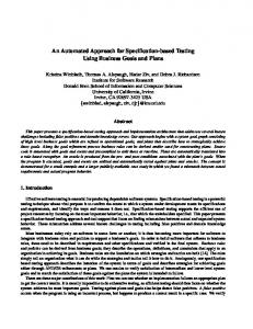
folded regions of the structure can exhibit structural variability across the ensemble. The approach of Swindells considers residues to contribute to a domain when they occur in regular secondary structure and have buried side chains that form predominantly hydrophobic contacts with one another. Again, this method is not entirely appropriate for identifying well defined regions across an ensemble of NMR-derived protein structures. An alternative approach to domain identification is suggested by work involving the analysis of protein conformational changes (Boutonnet et al., 1995). In this approach, (i) a pairwise comparison of two structures is performed, (ii) a rigid cut-off criterion is used for determining core versus non-core atoms and (iii) loops are not considered in defining the static core. Unfortunately, in the case of NMR-derived ensembles, (i) it is unclear how the method can be extended to consider an ensemble containing more than two structures, (ii) the diverse nature of NMR-derived ensembles makes the use of rigid cut-off criteria unappealing and (iii) as mentioned above, loop regions can often be well conserved across an ensemble and so their exclusion from the core would be inappropriate. Thus, in the context of NMR-derived ensembles of protein structures, it is useful to concentrate on spatially distinct regions of a protein whose local structure is conserved (i.e. behaves as a rigid body) across the ensemble. Subsequently, such regions will be referred to as ‘local structural domains’ (LSDs). We have recently developed a method for automatically clustering an ensemble of NMR-derived protein structures into conformationally related subfamilies (Kelley et al., 1996). This has laid the foundation for the current work: a computer program which automatically defines (i) the core atoms and (ii) the LSD(s) comprising the core, across an ensemble of structures. The method has the advantages that it does not use average structures, problems of rigid body superposition are avoided, cut-offs are a function of the particular ensemble and LSDs are determined automatically. This program, known as NMRCORE, is available via the World Wide Web (URL: http://neon.chem.le.ac.uk/). Materials and methods In brief, our approach uses the dihedral angle order parameter values (Hyberts et al., 1992) of all torsion angles followed by the application of a penalty function (Kelley et al., 1996) to define a core atom set. This atom set is then used as the starting point for an automated clustering procedure that uses inter-atom distances as its data set followed by the application of a second penalty function to determine the clustering cut-off position. This results in clusters of atoms each of which comprises a single LSD. An overview of the method is given in Figure 1. Step 1. Dihedral angle order parameter calculation To define the degree of order/disorder for each atom in the protein, the dihedral angle order parameter (OP) is used (Hyberts et al., 1992). Initially, all torsion angles in all members of the ensemble are calculated. The order parameter of each dihedral angle in each residue is then calculated in turn across the ensemble. The order parameter OP(αi) for the angle αi of residue i (where α 5 φ, ϕ, χ1 or χ2, etc.) is defined as OP(αi) 5

1 N

|

N

Σα

j i

j 5 1

|

where N is the total number of structures in the ensemble, 738

Fig. 1. Flow chart illustrating the progress of the NMRCORE algorithm.

αji (j 5 1, ..., N) is a 2D unit vector with phase equal to the dihedral angle αi, i represents the residue number and j stands for the number of the ensemble member. If the angle is the same in all structures, then OP has a value of 1, whereas a value for OP much smaller than 1 indicates a disordered region of the structure. NMRCORE generates a sorted list (ranked in decreasing order) of the OP values for every torsion angle (except ω) for every residue. This list is denoted OPlist .

Core and domain definition for NMR ensembles

Step 2. Defining a cut-off in the list of dihedral angle order parameter values A penalty function has been devised to define automatically a cut-off in OPlist . This function attempts to maximize the number of atoms considered to comprise the core whilst simultaneously maximizing the OP values (i.e. minimizing the dihedral angle disorder) in the list. The penalty value Pk for position k in the list is an extension of our previous work (in which such a function has been shown to work well; Kelley et al., 1996) and is calculated as follows: Pk 5

(T – 1) (OPk – OPmin) OPmax – OPmin

1k

where T is the total number of order parameters in OPlist , k 5 (1, ..., T), OPk is the order parameter at position k in the OPlist , OPmin is the last and smallest OP value in (the sorted) OPlist and OPmax is the first and largest OP value in OPlist . The maximum value of Pk (k 5 1, ..., T) is taken as the cut-off point. Thus, the cut-off is a function of the particular ensemble, rather than being a fixed (or ‘rigid’) parameter. All atoms corresponding to order parameters above the cut-off point in OPlist are taken as comprising the core. Step 3. Generation of inter-atom variance matrix For this and all subsequent steps, only the Cα atoms within the core are used by default (see Discussion). This Cα subset is denoted CAcore. For a given pair of Cα atoms a and b within CAcore, it is possible to calculate their distance from one another within each member of the ensemble. In an ensemble of N members, this will result in a set of distances [dj(a,b), j 5 1, ..., N], where dj(a,b) is the distance between atoms a and b in structure j. Using this set of distances it is possible to define the variance V(a,b) in their distance from one another across the ensemble: N

Σ (d (a,b) – d

2 avg(a,b))

j

V(a,b) 5

j51

N–1

where dj(a,b) is as defined above and davg(a,b) is the average distance between atoms a and b across the entire ensemble. In this way, every pairwise variance V(a,b) is calculated from the atoms within CAcore: V(a,b) (a 5 1, ..., Z); (b 5 1, ..., Z; b , a); (a,b ε CAcore) where Z is the total number of atoms within CAcore. Thus a symmetrical Z3Z matrix of variance values, VM, is formed. Step 4. Clustering of inter-atom variances The matrix of variances, VM, generated in step 3 can be used as input to a hierarchical clustering algorithm. The details of this clustering method have been described previously (Kelley et al., 1996). In brief, the method uses the average linkage clustering algorithm followed by the application of a penalty function to define automatically a cut-off in the clustering hierarchy; this cut-off is a function of the variances. The penalty function seeks to minimize simultaneously (i) the number of clusters and (ii) the spread across each cluster. The cut-off chosen (Kelley et al., 1996) then represents a state where the clusters are as highly populated as possible, whilst simultaneously maintaining the smallest spread. The smaller the spread of a cluster, the lower are the variances in the interatom distances of its members; the greater the population of

a cluster, the less likely is the chance of excluding atoms forming part of the same LSD. Step 5. Output of local structural domains Once a cut-off has been found in the clustering hierarchy, the clusters present at that point may be output to a file for later viewing. Each of these clusters consists of a set of atoms, all of whose pairwise inter-atom variances are low. Thus, a given cluster corresponds to a region of the structure whose internal distances are conserved across the ensemble and hence a single LSD. For example, in an α-helix with a flexible central residue [i.e. low OP(φ, ϕ) value] all residues except this central one will lie in the core. The N- and C-terminal halves of the helix will, however, lie in two different LSDs. Example applications To illustrate the performance of the program, its application to two proteins is presented: the oligomerization domain of the tumour suppressor p53 [Clore et al., 1995; deposited as Protein Data Bank (Abola et al., 1987) accession numbers 1SAE, 1SAG and 1SAI] and the HIV-1 nucleocapsid protein (Summers et al., 1992; 1AAF). These structures were chosen because they differ widely in the following respects: (i) numbers of residues, (ii) average number of NMR-derived restraints per residue and (iii) number of structures deposited. Tumour suppressor p53. The NMR solution structure of the oligomerization domain of the tumour suppressor p53 (1SAE,1SAG and1SAI) comprises a dimer of dimers. The structure contains a total of 164 residues, is based on 4472 experimental NMR restraints and is very well defined: the average pairwise ensemble r.m.s. over all Cα atoms of the 76 structures is 2.50 Å (0.3 Å for the well defined core backbone atoms). Using NMRCORE, one large LSD was identified (and four trivial LSDs comprising two residues each) consisting of residues 326–355 (Figure 2). This finding is in very close agreement with the authors, who identify the core region of the tetramer as residues 326–354. HIV-1 nucleocapsid protein. In contrast to the tumour suppressor p53, the HIV-1 nucleocapsid protein (1AAF) contains 55 residues, was determined from 191 NMR restraints and exhibits a high degree of variability across its ensemble of structures: the average ensemble r.m.s. over all Cα atoms of the 20 structures is 9.95 Å. Analysing the ensemble using NMRCORE, two LSDs were identified comprising (i) residues 15–21 and 23–31 and (ii) residues 36–39, 41–42 and 44–49. Note that residues 22, 40 and 43 exhibit a higher degree of conformational variability across the ensemble than those in the LSDs identified and are therefore excluded from our definition of the core. This observation is consistent with all three residues (22, 40 and 43) being glycine. These two LSDs are not simultaneously superposable because they are connected by a flexible linker region (residues 32–35). This is illustrated in Figure 3. The two LSDs identified automatically by NMRCORE are in very close agreement with the domains identified by the authors (residues 14–30 and 35–51, Summers et al., 1992), which correspond to N- and C-terminal zinc fingers, respectively. These two examples illustrate two important properties of the NMRCORE algorithm. First, the lack of a rigid cut-off criterion in defining the core atoms allows the algorithm to perform well with both relatively poorly defined (1AAF) and very well defined (1SAE, 1SAG and 1SAI) ensembles. Second, 739

L.A.Kelley, S.P.Gardner and M.J.Sutcliffe

Fig. 2. Cα trace for the A chain of the 76 models of the tumour suppressor p53 (1SAE, 1SAG, 1SAI) fitted on residues 326–355. The shaded region indicates the core as defined by NMRCORE. Only one of the four chains is shown for clarity.

in the case of the HIV-1 nucleocapsid protein (1AAF), the algorithm is shown to perform very well by identifying distinct LSDs exhibiting rigid body motion in close agreement with the authors’ definition. Flexibility of NMRCORE For each of the processes carried out by NMRCORE, the program can accept user-defined values to override its automatic calculations. The user may specify the dihedral angles used in step 1, the cut-off value used in step 2, atoms other than solely Cα atoms in step 3 and the cut-off used in the clustering in step 4. NMRCORE can also output the core atom set for use by the related program, NMRCLUST, for the automatic clustering of ensembles of structures into conformationally related subfamilies (Kelley et al., 1996). It can additionally output colour-coded LSDs for use by INSIGHT II (MSI, San Diego, CA, USA) for visual inspection. Discussion The default use of Cα atoms after core definition was chosen following findings (Gerstein and Altman, 1995) that essentially no difference is found in calculations using all heavy atoms from the use of Cα atoms alone. This was interpreted to indicate that Cα atoms alone were sufficient to define the essential features of the core. NMRCORE is fast. For example, in the case of the tumour suppressor p53 ensemble (1SAE, 1SAG and 1SAI) where 76 models have been deposited, each consisting of four chains of 41 residues each (i.e. 164 residues in total), NMRCORE 740

Fig. 3. Cα trace for 20 models of the HIV-1 nucleocapsid protein (1AAF) fitted on (a) residues 15–31 and (b) residues 36–49. In both parts, the LSDs identified by NMRCORE on which fitting has been performed are shaded in grey; the other LSD in each case is encircled by a black line. Note that each of the LSDs corresponds to a single zinc finger.

completed its analysis in 30 s on an SGI R4000. Also, NMRCORE is not restricted to ensembles of NMR-derived structures alone. It can also be used, for example, to define the core atoms and LSDs in ensembles of homology models (M.J.Sutcliffe, unpublished results) generated using a modelling program such as MODELLER (Sali and Blundell, 1993). In conclusion, the method described here can be used to define automatically a set of core atoms and their local structural domains across a set of structures, e.g. an ensemble of NMR-derived structures or an ensemble of homology models, rapidly and consistently, without the need for subjectively defined cut-offs. NMRCORE takes a file in PDB format containing an ensemble of structures as input and outputs a list of the atoms in each LSD. In addition, NMRCORE can take a series of user-defined parameters for full control over

Core and domain definition for NMR ensembles

the various calculations performed. The program is freely available via the World Wide Web (http://neon.chem.le.ac.uk/). Acknowledgements We thank Roman Laskowski and Janet Thornton for useful discussions. L.A.K. is supported by a BBSRC CASE studentship, sponsored by Oxford Molecular Ltd. M.J.S. is a Royal Society University Research Fellow.

References Abola,E.E., Bernstein,F.C., Bryant,S.H., Koetzle,T.F. and Weng,J. (1987) In Allen,F.H., Bergerhoff,G. and Sievers,R. (eds), Crystallographic Databases—Information Content, Software Systems, Scientific Applications. Data Commission of the International Union of Crystallography, Bonn, pp. 107–132. Billeter,M. (1992) Q. Rev. Biophys., 25, 325–377. Boutonnet,N.S., Rooman,M.J. and Wodak,S.J. (1995) J. Mol. Biol., 253, 633–647. Chothia,C. (1992) Nature, 357, 543–544. Clore,G.M., Ernst,J., Clubb,R., Omichinski,J.G., Poindexter Kennedy,W.M., Sakaguchi,K., Appella,E. and Gronenborn,A.M. (1995) Nature Struct. Biol., 2, 4. Gerstein,M. and Altman,R.B. (1995) J. Mol. Biol., 251, 161–175. Hyberts,S.G., Goldberg,M.S., Havel,T.F. and Wagner,G. (1992) Protein Sci., 1, 736–751. Kelley,L.A., Gardner,S.P. and Sutcliffe,M.J. (1996) Protein Engng, 9, 1063– 1065. Sali,A. and Blundell,T.L. (1993), J. Mol. Biol., 234, 779–815. Sowdhamini,R. and Blundell,T.L. (1995) Protein Sci., 4, 506–520. Summers,M.F. et al. (1992) Protein Sci., 1, 563. Sutcliffe,M.J. (1993) Protein Sci., 2, 936–944. Swindells,M.B. (1995) Protein Sci., 4, 103–112. Received November 14, 1996; revised January 27, 1997; accepted February 6, 1997

741