Protocols for optimal readout of qubits using a continuous quantum ...

Protocols for optimal readout of qubits using a continuous quantum nondemolition measurement Jay Gambetta,1 W. A. Braff,1 A. Wallraff,1, 2 S. M. Girvin,1 and R. J. Schoelkopf1

arXiv:cond-mat/0701078v2 [cond-mat.mes-hall] 24 Dec 2007

1

Departments of Applied Physics and Physics, Yale University, New Haven, CT 06520 2 Department of Physics, ETH Zurich, CH-8093 Zurich, Switzerland (Dated: February 6, 2008)

We study how the spontaneous relaxation of a qubit affects a continuous quantum non-demolition measurement of the initial state of the qubit. Given some noisy measurement record Ψ, we seek an estimate of whether the qubit was initially in the ground or excited state. We investigate four different measurement protocols, three of which use a linear filter (with different weighting factors) and a fourth which uses a full non-linear filter that gives the theoretically optimal estimate of the initial state of the qubit. We find that relaxation of the qubit at rate 1/T1 strongly influences the fidelity of any measurement protocol. To avoid errors due to this decay, the measurement must be completed in a time that decrease linearly with the desired fidelity while maintaining an adequate signal to noise ratio. We find that for the non-linear filter the predicted fidelity, as expected, is always better than the linear filters and that the fidelity is a monotone increasing function of the measurement time. For example, to achieve a fidelity of 90%, the box car linear filter requires a signal to noise ratio of ∼ 30 in a time T1 whereas the non-linear filter only requires a signal to noise ratio of ∼ 18. PACS numbers: 03.65.Yz, 03.67.Lx, 03.65.Wj, 89.70.+c

I.

INTRODUCTION

In this paper we consider the following problem. Given a qubit initially either in the ground or excited state with finite lifetime T1 , how can we best make use of a continuous-in-time noisy quantum non-demolition (QND) measurement to optimally estimate the initial state (ground or excited) of the qubit? A number of authors have previously considered the related problem of optimal estimation of the present state of the qubit based on the past and current measurement record [1, 2, 3, 4, 5, 6], but, to the best of our knowledge, the problem we consider here has not been previously studied. QND measurements play a central role in the theory and practical implementation of quantum measurements [7]. In a QND measurement, the interaction term in the Hamiltonian coupling the system to the measuring apparatus commutes with the quantity being measured, so that this quantity is a constant of the motion. This does not imply that the quantum state of the system is totally unaffected, but it does imply that the measurement is repeatable. For example, a Stern-Gerlach measurement of σ ˆz for a spin 1/2 particle initially prepared in an eigenstate of σ ˆx will randomly yield the results +1 and −1 with equal probability. However, all subsequent measurements of σ ˆz will yield exactly the same result as the initial measurement. The fact that QND measurements are repeatable is of fundamental practical importance in overcoming detector inefficiencies. A prototypical example is the electronshelving technique [8, 9] used to measure trapped ions. A related technique is used in present implementations of ion-trap based quantum computation. Here the (extremely long-lived) hyperfine state of an ion is read out

via state-dependent optical fluorescence. With properly chosen circular polarization of the exciting laser, only one hyperfine state fluoresces and the transition is cycling; that is, after fluorescence the ion almost always returns to the same state it was in prior to absorbing the exciting photon. Hence the measurement is QND. Typical experimental parameters [10] allow the cycling transition to produce N ∼ 106 fluorescence photons. Given the photomultiplier quantum efficiency and typically small solid angle coverage, only a very small number n ¯ d will be detected on average. The probability of getting zero detections (ignoring dark counts for simplicity) and hence misidentifying the hyperfine state is P (0) = e−¯nd . Even for a very poor overall detection efficiency of only 10−5 , we still have n ¯ d = 10 and nearly perfect fidelity F = 1 − P (0) ∼ 0.999955. It is important to note that the total time available for measurement is not limited by the phase coherence time (T2 ) of the qubit or by the measurement-induced dephasing [3, 4, 11, 12], but rather only by the rate at which the qubit makes real transitions between measurement (ˆ σz ) eigenstates. In a perfect QND measurement there is no measurement-induced state mixing [4] and the relaxation rate 1/T1 is unaffected by the measurement process. The ability to read out a qubit with high fidelity is of central importance to the successful construction of a quantum computer [13]. In order to successfully measure a qubit, its quantum state must be mapped into a piece of classical information by measuring the relative occupation of its two states with the highest possible fidelity. Possible qubit implementations include superconducting circuits, silicon based electron and nuclear spins, and trapped ions, among others [14, 15, 16, 17, 18, 19, 20, 21, 22, 23]. In order for qubits prepared in different states to be distinguishable, the measurement must be

2 completed before the excited qubits decay[4, 24]. Many atomic qubits have sufficiently long lifetimes so that relaxation is not a major concern [14, 16, 20], but most solid state qubits have lifetimes on the order of microseconds or less, and spontaneous relaxation plays a significant role in the measurement. The qubit relaxation affects different measurement schemes differently, but in all cases, it can limit the maximum fidelity. Although the behavior of a qubit during continuous measurement has been studied using Monte Carlo simulations [2, 3, 4, 5, 6], no attempt has been made to derive an analytical expression for the probability distribution of the initial state or to study how spontaneous emission impacts the measurement fidelity. This is at least partially because there exist very few high fidelity continuous QND measurements, and even fewer that operate in a regime where qubit relaxation is a limiting factor. With the application of low temperature amplifiers, high fidelity (though not necessarily weak continuous) measurements of superconducting qubits are now becoming feasible [19, 23, 25, 26, 27, 28, 29, 30, 31, 32]. These measurements have found asymmetries between the probability distributions for the integrated signal corresponding to the ground and excited states, but could not accurately predict them. Here we find that when we use a measurement protocol that only records the integrated signal, the qubit relaxation induces asymmetry in the probability distributions, and that with a sufficiently precise detector, the distributions become distinctly non-Gaussian. Unlike measurement of a perfect (i.e., non-decaying) qubit, where fidelity is always improved by a longer measurement, we show that there is some optimal measurement fidelity that depends on the signal to noise ratio (SNR) of the detector and the filter used. The first filter we consider is the linear box car filter and optimize over the integrated time tf . Choosing a longer or shorter integration time will lower the fidelity of the measurement. Next we show that by choosing a filter that gives exponentially less importance to results at later times slightly increases the fidelity. We then numerically find the optimal linear filter and compare these linear filters to a nonlinear filter that yields the theoretically optimal estimate of the initial state of the qubit given some measurement record Ψ. We find that we can reach the same fidelity as the linear filters at a substantially lower SNR. Furthermore, due to the nature of the updating protocol, the fidelity is a non-decreasing function of the measurement time. In summary, in this paper we determine the optimal measurement fidelity given four measurement protocols for continuous measurement experiments currently being performed, and also provides a guideline for the necessary detector signal to noise ratio in order to reach a particular desired fidelity in future experiments. There are two major ways of measuring qubits. The first method is a latching measurement, for example by having the qubit state modify the switching current (or state) of an adjacent Josephson junction [28, 29] or the

bifurcation point of the non-linear Josephson plasma oscillation [30, 31, 32]. In such latching measurements, the qubit is measured very quickly with very high signal to noise, and after only a short waiting time [15, 17, 28, 32]. Some versions of such strong measurements can in principle be QND [32]. The second method is to perform a sequence of repeated or weak continuous quantum non-demolition (QND) measurements, which each leave the populations of the qubit unchanged. Several recent experiments with solid-state qubits [23, 33, 34], have used continuous QND measurement schemes in which the qubit lifetime imposes the main limitation on the measurement fidelity, for which the analysis of this paper should apply. It is not just continuous measurements that are affected by qubit relaxation. For example, consider an idealized latching measurement scheme where a qubit is prepared in an eigenstate, but there is some finite arming time tarm before a perfect measurement is made. In this case, a qubit prepared in the ground state will always be measured correctly, but a qubit prepared in the excited state may have decayed during tarm and be misidentified. Thus if tarm is not infinitesimally small, the qubit lifetime places a limit on fidelity even with a perfect detector. II.

QUBIT WITH INFINITE LIFETIME

It is worthwhile to first consider the case when the qubit cannot relax from the state it is initially prepared in, so it is “fixed” for all time. This allows us to formalize our intuitive understanding of a general continuous measurement and to give us a result against which we can compare the finite lifetime case. We consider the measurement of a qubit with two states |+i (excited) and |−i (ground) and assume that the measurement result is given by the actual value of the qubit state plus Gaussian noise. This assumption is justified for example in the current circuit quantum electrodynamic experiments [11, 12, 22, 23] in which a cavity is dispersively coupled to the qubit (no energy is exchanged between the cavity and the qubit). A homodyne measurement on the cavity output will reveal the cavity state (which is proportional to σ ˆz ) plus Gaussian noise [12, 21]. This Gaussian noise will be at least the photon shot noise but in present experiments it is dominated by the following amplifier. In other words, the measurement is faithful and given that the system is in state i = ±1 our detector for a time interval dτ outputs ψ(τ ) with statistics r dτ SNR P (ψ|i) = exp[−(ψ − i)2 dτ SNR/2]. (2.1) 2π For convenience we have also introduced a dimensionless time τ = t/T1 where T1 is an arbitrary but finite number, that will become the relaxation lifetime when we treat the finite lifetime case. Here SNR is the ratio of integrated signal power to noise power. It is linear in the integration

time and we will adopt the convention of specifying the SNR as that achieved after integrating for time T1 . From this distribution we can write ψ(τ ) in terms of the Wiener increment dW (τ ) [35] as p ψ(τ )dτ = i± (τ )dτ + SNR−1 dW (τ ). (2.2)

Here we have introduced the subscript ± to indicate a possible realization of the dynamics of the qubit given the initial condition ±1. For this case the qubit can be initialized in either state, but because it has an infinite lifetime, it is fixed in whatever state it starts in for the duration of the measurement. That is, i± (τ ) = ±1. We define our measurement signal s as the output of the detector integrated over time τf Z τf dτ ψ(τ ). (2.3) s= 0

Formally we are restricting ourselves here to a simple box car linear filter which uniformly weights the measurement record ψ(τ ) in the interval 0 < τ < τf . Using Eq. (2.2) it is simple to carry out the above integral and rewrite the measurement signal as s± (τf ) = ±τf + XG [0, σ 2 ] where XG [0, σ 2 ] is a Gaussian p random variable of mean 0 and standard deviation σ = τf /SNR. The signals then follow the familiar Gaussian distributions P±fixed (s) =

2 2 1 √ e−(s∓τf ) /(2σ ) . σ 2π

(2.4)

Because these distributions are symmetric about s = 0, the most obvious analysis is to set a signal threshold νth = 0 and call every measurement with s > νth a (+1) state, and every measurement with s < νth a (−1) state. Calculation of fidelity in this case is accomplished using the definition

F ≡ 1−

Z

νth

−∞

ds P+ (s) −

Z

∞ νth

ds P− (s).

(2.5)

For the case of infinite qubit lifetime we have the simple result ! r τf SNR F = erf . (2.6) 2 A fidelity of zero corresponds to a completely random measurement that extracts no information, a fidelity of one corresponds to a perfect faithful measurement, and in between the measurement conveys varying degrees of certainty. As τf becomes large, Eq. (2.5) predicts that the fidelity rapidly approaches unity. Higher SNR serves to speed up the convergence, but as long as SNR is non zero, any desired fidelity is attainable simply by measuring the qubit for long enough. In Table I, the required SNRfixed is listed in order to achieve a given fidelity within T1 . Note the same results for the fidelity would be obtained if we used the optimal non-linear filter of Sec. VI. That is, for

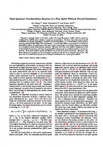
Detector output, s(o)

3 2 1 0