Hydrol. Earth Syst. Sci., 21, 4879–4893, 2017 https://doi.org/10.5194/hess-21-4879-2017 © Author(s) 2017. This work is distributed under the Creative Commons Attribution 3.0 License.
Providing a non-deterministic representation of spatial variability of precipitation in the Everest region Judith Eeckman1 , Pierre Chevallier1 , Aaron Boone2 , Luc Neppel1 , Anneke De Rouw3 , Francois Delclaux1 , and Devesh Koirala4 1 Laboratoire
HydroSciences (CNRS, IRD, Université de Montpellier) CC 57 – Université de Montpellier 163, rue Auguste Broussonnet 34090 Montpellier, France 2 CNRM UMR 3589, Météo France/CNRS, Toulouse, France 3 Institut de Recherche pour le Développement, Université Pierre et Marie Curie, 4 place Jussieu, 75252 Paris CEDEX 5, France 4 Nepal Academy of Science and Technology, G.P.O. box 3323, Khumaltar, Lalitpur, Nepal Correspondence to: Judith Eeckman (
[email protected]) Received: 9 March 2017 – Discussion started: 17 May 2017 Revised: 3 August 2017 – Accepted: 4 August 2017 – Published: 28 September 2017
Abstract. This paper provides a new representation of the effect of altitude on precipitation that represents spatial and temporal variability in precipitation in the Everest region. Exclusive observation data are used to infer a piecewise linear function for the relation between altitude and precipitation and significant seasonal variations are highlighted. An original ensemble approach is applied to provide non-deterministic water budgets for middle and high-mountain catchments. Physical processes at the soil– atmosphere interface are represented through the Interactions Soil–Biosphere–Atmosphere (ISBA) surface scheme. Uncertainties associated with the model parametrization are limited by the integration of in situ measurements of soils and vegetation properties. Uncertainties associated with the representation of the orographic effect are shown to account for up to 16 % of annual total precipitation. Annual evapotranspiration is shown to represent 26 % ± 1 % of annual total precipitation for the mid-altitude catchment and 34% ± 3 % for the high-altitude catchment. Snowfall contribution is shown to be neglectable for the mid-altitude catchment, and it represents up to 44 % ± 8 % of total precipitation for the highaltitude catchment. These simulations on the local scale enhance current knowledge of the spatial variability in hydroclimatic processes in high- and mid-altitude mountain environments.
1
Introduction
The central part of the Hindu Kush Himalaya region presents tremendous heterogeneity, in particular in terms of topography and climatology. The terrain ranges from the agricultural plain of Terai to the highest peaks of the world, including Mount Everest, over a south–north transect about 150 km long (Fig. 1). Two main climatic processes on the synoptic scale are distinguished in the central Himalayas (Barros et al., 2000; Kansakar et al., 2004). First, the Indian monsoon is formed when moist air arriving from the Bay of Bengal is forced to rise and condense on the Himalayan barrier. Dhar and Rakhecha (1981) and Bookhagen and Burbank (2010) assessed that about 80 % of annual precipitation over the central Himalayas occurs between June and September. However, the timing and intensity of this summer monsoon is being reconsidered in the context of climate change (Bharati et al., 2016). The second main climatic process is a west flux that gets stuck in appropriately oriented valleys and occurs between January and March. Regarding high altitudes (> 3000 m), this winter precipitation can occur exclusively in solid form and can account for up to 40 % of annual precipitation (Lang and Barros, 2004) with considerable spatial and temporal variation.
Published by Copernicus Publications on behalf of the European Geosciences Union.
4880
J. Eeckman et al.: Providing a representation of precipitation in the Everest region
On a large spatio-temporal scale, precipitation patterns over the Himalayan Range are recognized to be strongly dependent on topography (Anders et al., 2006; Bookhagen and Burbank, 2006; Shrestha et al., 2012). The main thermodynamic process is an adiabatic expansion when air masses rise, but, at very high altitudes (> 4000 m), the reduction of available moisture is a concurrent process. Altitude thresholds of precipitation can then be discerned (Alpert, 1986; Roe, 2005). However, this representation of orographic precipitation has to be modulated considering the influence of such a protruding relief (Barros et al., 2004). Products for precipitation estimation currently available in this area, e.g. the APHRODITE interpolation product (Yatagai et al., 2012) and the Tropical Rainfall Measuring Mission (TRMM) remote product (Bookhagen and Burbank, 2006), do not represent spatial and temporal variability in orographic effects at a resolution smaller than 10 km (GongaSaholiariliva et al., 2016). Consequently, substantial uncertainty remains in water budgets simulated for this region, as highlighted by Savéan et al. (2015). In this context, groundbased measurements condensed in small areas have been shown to enhance the characterization of local variability in orographic processes (Andermann et al., 2011; Pellicciotti et al., 2012; Immerzeel et al., 2014). However, although the Everest region is one of the most closely monitored areas of the Himalayan Range, valuable observations remain scarce. In particular, the relation between altitude and precipitation is still poorly documented. The objective of this paper is to provide a representation of the effect of altitude on precipitation that represents spatial and temporal variability in precipitation in the Everest region. The parameters controlling the shape of the altitudinal factor are constrained through an original sensitivity analysis step. Uncertainties associated with variables simulated through the Interactions Soil–Biosphere–Atmosphere (ISBA) surface scheme (Noilhan and Planton, 1989) are quantified. The first section of the paper presents the observation network and recorded data. The second section describes the model chosen to represent orographic precipitation, including computed altitude lapse rates for air temperature and precipitation. The method for statistical analysis through hydrological modelling is also described. The third section presents and discusses the results of sensitivity analysis and uncertainty analysis.
2 2.1
Data and associated uncertainties Meteorological station transect
stations are located to depict the altitudinal profile of P and T over (1) the main river valley (Dudh Kosi Valley), oriented south–north, and (2) the Kharikhola tributary river, oriented east–west. To reduce undercatching of solid precipitation, two Geonors® were installed at 4218 and 5035 m in 2013. Measurements at Geonor® instrumentation allow us to correct the effect of wind and the loss of snowflakes. Records from four other stations administrated by the Ev-K2-CNR association (www.evk2cnr.org) are also available. Total precipitation, air temperature, atmospheric pressure (AP), relative humidity (RH), wind speed (WS), short-wave radiation (direct and diffuse) (SW) and long-wave radiation (LW) have been recorded with an hourly time step since 2000 at Pyramid station (5035 m a.s.l.). Overall, these 10 stations cover an altitude range from 2078 m to 5035 m a.s.l., comprising a highly dense observation network, compared to the scarcity of ground-based data in this type of environment. The characteristics of the 10 stations are summarized Table 1. The meteorological data provided by the EVK2-CNR association are available by contacting the respective authors. All other data used in this study are freely available through the platform www.papredata.org. Annual means of temperature and precipitation measured at these stations are presented are Table 2 for the two hydrological years 2014–2015 and 2015–2016. These time series contain missing data periods, which can represent up to 61 % of the recorded period. For stations LUK, NAM, PHA, PAN, PHE and PYR, where relatively long time series are available, gaps were filled with the interannual hourly mean for each variable. For the other stations, gaps were filled with values at the closest station, weighted by the ratio of mean values over the common periods. Time series from 1 January 2013 to 30 April 2016 were then reconstructed from these observations. Two seasons are defined based on these observations and knowledge of the climatology of the central Himalayas: (1) the monsoon season, from April to September, including the early monsoon, whose influence seems to be increasing with the current climate change (Bharati et al., 2014); (2) the winter season, dominated by westerly entrances with a substantial spatio-temporal variability. Local measurements cannot be an exact quantification of any climatic variables, and they are necessarily associated with errors that follow an random distribution law. In particular, snowfall is usually undercaught by instrumentation (Sevruk et al., 2009). However, since this study focuses most particularly on uncertainty associated with spatialization of local measurements, aleatory errors in measurements will not be considered here.
An observation network of 10 stations (Table 1 and Fig. 1) records hourly precipitation (P ) and air temperature (T ) since 2010 and 2014. The stations are equipped with classical rain gauges and HOBO® sensors for temperature. The Hydrol. Earth Syst. Sci., 21, 4879–4893, 2017
www.hydrol-earth-syst-sci.net/21/4879/2017/
J. Eeckman et al.: Providing a representation of precipitation in the Everest region
4881
Table 1. Overview of the observation network used in this study. Air temperature (T ), precipitation (P ) atmospheric pressure (AP), relative humidity (RH), wind speed (WS), and short- and long-wave radiation (SW, LW) are recorded on an hourly timescale. The Geonor® at the Pyramid and Pheriche stations record total precipitation (PGEO ) on an hourly timescale. The two hydrometric stations at Kharikhola and Pangboche have been recording water level since 2014. ID
Station
Altitude m a.s.l.
Latitude
Longitude
Period (date format: yyyy-mm-dd)
Measured variable
KHA MER BAL PHA LUK PAR TCM NAM PAN PHE
Kharikhola Mera School Bhalukhop Phakding Lukla Paramdingma Pangom Namche Pangboche Pheriche
2078 2561 2575 2619 2860 2869 3022 3570 3976 4218
27.60292 27.60000 27.60097 27.74661 27.69694 27.58492 27.58803 27.80250 27.85722 27.89528
86.70311 86.72269 86.74017 86.71300 86.72270 86.73956 86.74828 86.71445 86.79417 86.81889
PYR
Pyramid
5035
27.95917
86.81333
2014-05-03 2014-05-02 2014-05-03 2010-04-07 2002-11-02 2014-05-03 2014-05-03 2001-10-27 2010-10-29 2001-10-25 2012-12-06 2000-10-01
2015-10-28 2015-10-28 2015-10-28 2016-05-16 2016-01-01 2015-10-28 2015-10-28 2016-01-01 2016-05-08 2016-01-01 2016-05-16 2016-01-01
668.7 668.03
Kharikhola Pangboche
1985 3976
27.60660 27.85858
86.71847 86.79253
2016-04-26 2014-05-03 2014-05-17
2016-04-26 2016-05-20 2016-05-09
P,T P,T P,T P,T P,T P,T P,T P,T P,T T PGEO T , AP, RH, WS, LW, SW PGEO Water level Water level
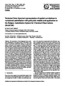
Figure 1. Map of the monitored area: the Dudh Kosi River basin at the Rabuwabazar station, managed by the Department of Hydrology and Meteorology, Nepal Government (station coordinates: 27◦ 160 0900 N, 86◦ 400 0300 E; station elevation: 462 m a.s.l.; basin area: 3712 km2 ). The Tauche and Kharikhola subcatchments are defined by the corresponding limnimetric stations.
2.2
Discharge measurement stations and associated hydrological catchments
Two hydrometric stations were equipped with Campell® hydrometric sensors and encompass two subbasins: the Kharikhola catchment (18.2 km2 ) covers altitudes from 1900 to 4450 m (mid-altitude mountain catchment), and Tauche www.hydrol-earth-syst-sci.net/21/4879/2017/
catchment (4.65 km2 ) altitudes range from 3700 to 6400 m (high-altitude mountain catchment). Water level time series are available from March 2014 to March 2015. The time series at Kharikhola station contains 34 % of missing data in 2014–2015, corresponding to damage to the sensor (Table 3). Uncertainty in discharge is usually considered to account for less than 15 % of discharge (Lang et al., 2006). Hydrol. Earth Syst. Sci., 21, 4879–4893, 2017
4882
J. Eeckman et al.: Providing a representation of precipitation in the Everest region
Recession times are computed for available recession periods using the lfstat R library (Koffler and Laaha, 2013) with both the recession curves method (World Meteorological Organization, 2008) and the base flow index method (Chapman, 1999). We found recession times for Kharikhola and Tauche catchments of, respectively, around 70 days and around 67 days. Consequently, we consider that there is no interannual storage in either of the two catchments. This hypothesis can be modulated if a contribution of deep groundwater is considered (Andermann et al., 2011). Since these two catchments have no (Kharikhola) or neglectable (Tauche) glacier contribution, we hypothesized that the only entrance for water budgets in these catchments is total precipitation. In this study we used these two catchments as samples to assess generated precipitation fields against observed discharge on the local scale. The hydrological year is considered to start on 1 April, as decided by the Department of Hydrology and Meteorology of the Nepalese Government and generally accepted (Nepal et al., 2014; Savéan et al., 2015). 3
3.1
Spatialization methods for temperature and precipitation Temperature
In mountainous areas, temperature and altitude generally correlate well linearly, considering a large timescale (Valéry et al., 2010; Gottardi et al., 2012). In the majority of studies based on field observations, air temperature values are extrapolated using the inverse distance weighting method (IDW) (Andermann et al., 2012; Immerzeel et al., 2012; Duethmann et al., 2013; Nepal et al., 2014). An altitude lapse rate θ (in ◦ C km−1 ) is also used to take altitude into account for hourly temperature computation at any point M of the mesh extrapolated by IDW: X d −1 (M, Si ) · (T (Si ) + θ · (zm − zi )) T (M) =
Si
X d −1 (M, Si )
,
(1)
Si
where T is the hourly temperature, Si the ith station of the observation network, zi the altitude of station Si , zM the altitude of grid point M, and d −1 is the inverse of distance in latitude and longitude. In the Himalayas, seasonal (Nepal et al., 2014; Ragettli et al., 2015) or constant (Pokhrel et al., 2014) altitudinal lapse rates (LRs) are used for temperature. Figure 2 presents seasonal LRs computed from temperature time series at the 10 stations described in Sect. 2.1. The linearity is particularly satisfying for both seasons, even if stations follow differently oriented transects (W–E or N–S orientation). Computed LRs for both seasons are very close to values proposed by Immerzeel et al. (2014) and Heynen Hydrol. Earth Syst. Sci., 21, 4879–4893, 2017
Figure 2. Linear regression for measured seasonal temperatures for the winter and monsoon seasons. Points (circles or triangles) are the seasonal means at each monitored station. Altitude lapse rates are displayed for each season in ◦ C km−1 .
et al. (2016) (Langtang catchment; 585 km2 ; elevation ranging from 1406 to 7234 m a.s.l.) and Salerno et al. (2015) (Kosi Basin; 58 100 km2 ; from 77 m a.s.l. to 8848 m a.s.l.). Consequently, these values for seasonal LRs will be used in this study. Uncertainties associated with temperature interpolation will therefore be neglected because they have minor impact on modelling compared to uncertainties in precipitation. 3.2 3.2.1
Precipitation Model of orographic precipitation
The complexity of precipitation spatialization methods has been commented on by Barros and Lettenmaier (1993). When orographic effects are not well understood, complex approaches do not necessarily reproduce local measurements efficiently (Bénichou and Le Breton, 1987; Frei and Schär, 1998; Daly et al., 2002). In the central Himalayas, various hydrologic and glaciological studies are based on observation networks to produce a precipitation grid. However, few studies provide precipitation fields on an hourly timescale (Ragettli et al., 2015; Heynen et al., 2016), and precipitation fields on spatial scales lower than 1 km are always obtained using altitude linear lapse rates (Immerzeel et al., 2012; Nepal et al., 2014; Pokhrel et al., 2014). However, the considered lapse rates are constant in time and/or uniform in space. The spatial and temporal variability in the precipitation is then not represented in these studies. Moreover, the geostatistical co-kriging method has been applied by GongaSaholiariliva et al. (2016) for monsoon precipitation interpolation over the Kosi catchment. However, the provided precipitation fields overall underestimate the observations, and this method is shown not to be adequate for the interpolation of solid precipitation. The IDW method is a simple, widely www.hydrol-earth-syst-sci.net/21/4879/2017/
J. Eeckman et al.: Providing a representation of precipitation in the Everest region
4883
Table 2. Overview of measurements at meteorological stations used in this study over the hydrological years 2014–2015 and 2015–2016. T and P stand for, respectively, annual mean temperature and annual total precipitation. T and P are computed for time series completed with either a weighted value at the closest station when available or their respective interannual mean. 2014–2015 Temperature Station
Precipitation
Gaps
T ◦C
KHA MER BAL PHA LUK PAR TCM NAM PAN PHE PYR
13.96 13.44 9.92 9.26 10.18 7.98 7.07 5.09 3.81 0.80 −2.71
2015–2016
0.1 % 12.4 % 15.1 % 41.9 % 54.5 % 20 % 21.1 % 19.9 % 0.2 % 61 % 18.6 %
P mm
Gaps
2453 3241 3679 1664 2278 3592 3592 964 876 701 701
34.5 % 12.2 % 34.4 % 0.0 % 41.8 % 19.8 % 20.8 % 0.1 % 0.0 % 0.0 % 0.0 %
Station Kharikhola Pangboche
2015–2016
Q mm
Gaps
Q mm
Gaps
2341 416
34.0 % 0.0 %
1746 499
0.0 % 0.0 %
used method to spatialize precipitation in mountainous areas (Valéry et al., 2010; Gottardi et al., 2012; Duethmann et al., 2013; Nepal et al., 2014). In the French Alps, Valéry et al. (2010) combine the IDW method with a multiplicative altitudinal factor. Precipitation at any point M of the mesh extrapolated by the IDW is given by X d −1 (M, Si ) · (P (Si ) exp(β(zM − zi )) P (M) =
Si
X d −1 (M, Si )
.
(2)
Si
In Eq. (2), the altitude effect is represented through the introduction of the altitudinal factor β, defined by Valéry et al. (2010) as the slope of the linear regression between the altitude of stations (in m a.s.l.) and the logarithm of the seasonal volume of total precipitation expressed in millimetres. This method presents the advantage of using an altitudinal factor which can vary in time and space. The spatial and temporal variability in the precipitation is therefore represented in this method. Moreover, the effect of altitude is independently www.hydrol-earth-syst-sci.net/21/4879/2017/
T 15.50 14.83 10.48 9.16 10.19 7.84 6.90 5.17 4.20 0.84 −2.30
Precipitation
Gaps
P mm
Gaps
100 % 100 % 0.0 % 0.0 % 40 % 100 % 100 % 57.9 % 0.0 % 8.6 % 9.3 %
1752 2278 2628 1226 2278 2540 2628 788 526 526 438
100 % 100 % 0.0 % 0.0 % 0.2 % 100 % 100 % 0.1 % 0.0 % 0.0 % 0.0 %
◦C
Table 3. Overview of measurements at hydrological stations used in this study over the hydrological years 2014–2015 and 2015– 2016. Q stands for annual discharge. Q for the Kharikhola station in 2014–2015 is completed with the interannual mean. 2014–2015
Temperature
studied and the controlling parameters have physical meaning. 3.2.2
Observed relation between altitude and seasonal precipitation
Several studies based on observations (Dhar and Rakhecha, 1981; Barros et al., 2000; Bookhagen and Burbank, 2006; Immerzeel et al., 2014; Salerno et al., 2015) or theoretical approaches (Burns, 1953; Alpert, 1986) have observed that precipitation in the Himalayan Range generally presents a multimodal distribution along elevation. Precipitation is considered to increase with altitude until a first altitudinal threshold located between 1800 and 2500 m, depending on the study, and to decrease above 2500 m. Moreover, the linear correlation of precipitation with altitude is reported to be weak for measurements above 4000 m (Salerno et al., 2015). The decreasing of precipitation with altitude is characterized through various functions (Dhar and Rakhecha, 1981; Bookhagen and Burbank, 2006; Salerno et al., 2015). Nevertheless, the hypothesis of linearity of precipitation (P ) with altitude (z) is often made with a constant (Nepal et al., 2014) or time-dependent lapse rate (Immerzeel et al., 2014). Gottardi et al. (2012) noted that, in mountainous areas, the hypothesis of a linear relation between P and z is only acceptable over a small spatial extension and for homogeneous weather types. Consequently, we considered altitude lapse rates for precipitation on the seasonal timescale, and we analysed the spatial variability in the relation between P and z. For this purpose, we chose to regroup the stations into three groups (see Fig. 1): (1) stations with elevation ranging from 2078 to 3022 m, following a west–east transect (Group 1); (2) stations with elevation ranging from 2619 to Hydrol. Earth Syst. Sci., 21, 4879–4893, 2017
4884
J. Eeckman et al.: Providing a representation of precipitation in the Everest region
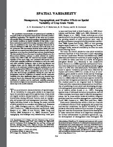
3570 m following a south-westerly transect (Group 2); and (3) stations with elevation above 3970 m (Group 3). Figure 3 shows that for Group 1, observed seasonal volumes of precipitation increase globally with altitude at a rate lower than 0.1 km−1 ; for Group 2, seasonal volumes decrease at a rate around −0.3 km−1 ; for Group 3, seasonal volumes decrease at a rate lower than 0.2 km−1 , with a poor linear trend. The overlapping of altitude ranges between Group 1 and Group 2 highlights that the relation between precipitation and altitude strongly depends on terrain orientation. The difference in seasonal volumes at the BAL (2575 m a.s.l., 3471 mm year−1 ) and MER stations (2561 m a.s.l., 2245 mm year−1 ) (GROUP 1) also results from site effects on precipitation. In summary, β values inferred from local observations mainly express local variability and are not sufficient to establish any explicit relation between precipitation and altitude on the catchment scale. However, for operational purposes, the β factor can be simplified as a multimodal function of altitude within the Dudh Kosi catchment. The β factor is represented as a piecewise linear function of altitude using two altitude thresholds (z1 and z2 ) and three altitude lapse rates (β1 , β2 and β3 ): z ≤ z1 β1 > 0 if β2 < 0 if z1 < z ≤ z2 . β(z) = (3) β3 ∼ 0 if z > z2 . As no deterministic value can be ensured for the five parameters controlling the shape of Eq. (3), an ensemble approach was applied (see Sect. 4) to estimate parameter sets on the scale of the entire Dudh Kosi River basin that are optimally suitable for both the Tauche and the Kharikhola catchments. 4 4.1
Sensitivity and uncertainties analysis method Overall strategy
Saltelli et al. (2006) distinguishes between sensitivity analysis (SA), which does not provide a measurement of error, and uncertainties analysis (UA), which computes a likelihood function according to reference data. SA is run before UA as a diagnostic tool, in particular to reduce variation intervals for parameters and therefore save computation time. The algorithm chosen for SA was the regional sensitivity analysis (RSA) (Spear and Hornberger, 1980) method. The RSA method is based on the separation of the parameter space into (at least) two groups: behavioural or nonbehavioural parameter sets. A behavioural parameter set is a set that respects conditions (maximum or minimum thresholds) on the output of the orographic precipitation model. Thresholds will be defined for solid and total precipitation in the “Results and discussion” section. The analysis is performed using the R version of the SAFE(R) toolbox, developed by Pianosi et al. (2015). Hydrol. Earth Syst. Sci., 21, 4879–4893, 2017
SA and UA are set up as follows (Beven, 2010): 1. First, the parameter space is sampled, according to a given sampling distribution. For each parameter set, hourly precipitation fields are computed at the 1 km resolution using Eq. (2) for both the Tauche and the Kharikhola catchments. Since physical processes strongly differ between the winter and monsoon seasons, we chose to differentiate the altitude correction for the two seasons. Behavioural parameter sets were then selected for each of the two seasons. 2. Then, for each behavioural precipitation field, the ISBA surface scheme, described in the next section, was run separately on Kharikhola and Tauche catchments. The objective function was computed as the difference between simulated and observed annual discharge at the outlet of each catchment. Parameter sets that lead to acceptable discharge regarding observed discharge for the two catchments are finally selected. 4.2 4.2.1
Hydrological modelling on the local scale The ISBA surface scheme
We considered that there was no interannual storage in either of the two subcatchments studied; i.e. the variation in the groundwater content was considered zero from one hydrological year to the other. Consequently, annual simulated discharges were computed as the sum over all grid cells and all time steps of simulated surface flow and simulated subsurface flow. The question of the calibration of flow routing in the catchment was thus avoided. The ISBA surface scheme (Noilhan and Planton, 1989; Noilhan and Mahfouf, 1996) simulates interactions between the soil, vegetation and the atmosphere with a sub-hourly time step (SVAT model). The multilayer version of ISBA (ISBA-DIF) uses a diffusive approach (Boone et al., 2000; Decharme et al., 2011): surface and soil water fluxes are propagated from the surface through the soil column. Transport equations for mass and energy are solved using a multilayer vertical discretization of the soil. The explicit snow scheme in ISBA (ISBA-ES) uses a three-layer vertical discretization of snowpack and provides a mass and energy balance for each layer (Boone and Etchevers, 2001). Snowmelt and snow sublimation are taken into account in balance equations. The separation between runoff over saturated areas (Dunne runoff), infiltration excess runoff (Horton runoff) and infiltration is controlled by the variable infiltration capacity scheme (VIC) (Dümenil and Todini, 1992). The ISBA code is freely available from the respective authors. The precipitation phase was estimated depending on hourly air temperature readings. Mixed phases occurred for temperatures between 0 and 2 ◦ C, following a linear relation. Other input variables required for ISBA (atmospheric pressure, relative humidity, wind speed, short- and long-wave rawww.hydrol-earth-syst-sci.net/21/4879/2017/
J. Eeckman et al.: Providing a representation of precipitation in the Everest region
4885
Figure 3. Piecewise relation between altitude and the logarithm of observed seasonal volumes of total precipitation, separated by season and station group. Seasonal values for β (km−1 ) are computed from observed precipitation for each of the three station groups.
diations) were interpolated from measurements at Pyramid station as functions of altitude, using the method proposed by Cosgrove et al. (2003). Short-wave radiation and wind speed are not spatially interpolated and are considered to be equals to the measurements at Pyramid station for the two catchments. 4.2.2
Parametrization of surfaces
Several products provide parameter sets for physical properties of surfaces on the global scale (Hagemann, 2002; Masson et al., 2003; Arino et al., 2012). However, these products are not accurate enough at the resolution required for this study. The most recent analysis (Bharati et al., 2014; Ragettli et al., 2015) exclusively used knowledge garnered from the literature. To detail the approach, in this study the parametrization was based on in situ measurements. A classification into nine classes of soil/vegetation entities was defined based on Sentinel-2 images at a 10 m resolution (Drusch et al., 2012), using a supervised classification tool of the QGIS Semi-Automatic Classification Plugin (Congedo, 2015). In and around the two catchments, 24 reference sites were sampled during field missions. Data collection included soil texture, soil depth and root depth, determined by augering to a maximum depth of 1.2 m. Vegetation height and structure and dominant plant species were also determined. The results were classified into nine surface types. The nine classes and their respective fractions in the Kharikhola and Tauche catchments are presented Table 4. Analysis of soil samples showed that soils were mostly sandy (∼ 70 %), with a small proportion of clay (∼ 1 %). Soil depths varied from very thin (∼ 30 cm) at high altitudes to 1.2 m for flat cultivated areas. Forest areas were separated into three classes: dry forests were characterized by high slopes and shallow soils; wet forests presented deep silty www.hydrol-earth-syst-sci.net/21/4879/2017/
Figure 4. Classification of surfaces defined for the two Kharikhola and Tauche subcatchments, established using the supervised classification tool of the QGIS Semi-Automatic Classification Plugin (Congedo, 2015), based on Sentinel-2 images at a 10 m resolution (Drusch et al., 2012). In situ sample points were used to describe the soil and vegetation characteristics of each class.
soils (1 m), with high trees (7 m); intermediate forests had moderate slopes and relatively deep, sandy soils. Crop areas presented different soil depths depending on their average slope. In addition, values for unmeasured variables (leaf area index (LAI), soil and vegetation albedos, surface emissivity, surface roughness) were taken from the ECOCLIMAP1 classification (Masson et al., 2003) for ecosystems representative of the study area. ECOCLIMAP1 provides the annual cycle of dynamic vegetation variables, based both on a surface properties classification (Hagemann, 2002) and on a global climate map (Koeppe and De Long, 1958). The ECOCLIMAP2 product (Faroux et al., 2013) is derived from ECOCLIMAP1 and provides enhanced descriptions of surfaces. However, ECOCLIMAP2 is only available for Europe and therefore is not used in this study. Hydrol. Earth Syst. Sci., 21, 4879–4893, 2017
4886
J. Eeckman et al.: Providing a representation of precipitation in the Everest region
Table 4. Soil and vegetation characteristics of the nine classes defined in the Kharikhola and Tauche catchments; “% KK” and “% Tauche” represent the fraction of each class in the Kharikhola and Tauche catchments. Sand and clay fractions (“% Sand” and “% Clay”, respectively), soil depth (SD), root depth (RD), and tree height (TH) are defined based on in situ measurements. The dynamic variables (e.g. the fraction of vegetation and leaf area index) are found in the ECOCLIMAP1 classification (Masson et al., 2003) for representative ecosystems.
5
ID
Class
1 2 3 4 5 6 7 8 9
Snow and ice Screes Steppe Shrubs Dry forest Intermediary forest Wet forest Slope terraces Flat terraces
% KK
% Tauche
% Sand
% Clay
TH m
SD m
RD m
ECOCLIMAP1 cover
– 3.1 % 0.6 % 7.4 % 9.7 % 45.7 % 20.6 % 11.2 % 1.4 %
0.7 % 31.2 % 33.7 % 34.4 % – – – – –
0.00 0.00 81.41 70.60 72.86 84.97 70.12 70.89 67.01
0.00 0.00 1.70 1.55 1.00 1.01 1.00 1.38 1.69
0.0 0.0 0.0 0.0 12.0 27.5 6.8 5.6 2.5
0.00 0.00 0.10 0.35 0.20 0.42 1.04 0.56 1.267
0.00 0.00 0.10 0.27 0.20 0.40 0.50 0.26 0.20
6 5 123 86 27 27 27 171 171
Results and discussion
5.1
Regional sensitivity analysis
The parameter space was sampled using the “All at a time” (AAT) sampling algorithm from the SAFE(R) toolbox (Pianosi et al., 2015). Since no particular information was available on prior distribution and interaction for the five parameters, uniform distributions were considered. The size of parameter samples was chosen according to Sarrazin et al. (2016) (Table 5). The optimization method is highly sensitive to the choice of initial values for the β1 , β2 , β3 , z1 and z2 parameters. Several attempts have been made, and the choices presented Table 6 are justified by the following arguments: – Minimum and maximum values for the altitude thresholds z1 and z2 are chosen according to both literature review (Barros et al., 2000; Anders et al., 2006; Bookhagen and Burbank, 2006; Shrestha et al., 2012; Nepal, 2012; Savéan, 2014) and observations. The first inquired altitudinal threshold is described in the literature as between 2000 and 3000 m, and the second threshold is described as above 4000 m. These intervals have been enlarged to also test related values. – Maximum (minimum) values for β1 (β2 ) are chosen about 10 times larger than the value computed based on observation. Considering the definition of the beta coefficient, a value greater than 2 km−1 (lower than −2 km−1 ) would lead to a multiplication of precipitation by 1.22 (by 0.82) within 100 m. When applied to the precipitation observed at stations, this would lead to inconsistent precipitation when increasing altitude by 100 m. – The β3 coefficient has to be negative because a positive value would lead to unrealistic values at high altitudes. Moreover, the minimum value is chosen to be significantly smaller than the value computed for β3 based on Hydrol. Earth Syst. Sci., 21, 4879–4893, 2017
the observations but also to remain higher than the value computed for β2 based on the observations. A behavioural parameter set is a set that leads to an annual amount of total precipitation for both catchments comprised between a minimum and a maximum value. A parameter sets that does not meet these conditions is considered as nonbehavioural. Maximum and minimum conditions on annual total precipitation for a set to be behavioural were chosen according to the annual observed discharge for each of the two catchments. The mean observed discharge for the recorded period was 2043 mm year−1 at the Kharikhola station and 457 mm year−1 at the Tauche station. Annual total precipitation was expected to be greater than the measured annual discharge and lower than annual discharge plus 70 %. These thresholds take into account both the uncertainty in measured discharges and actual evapotranspiration. Based on values proposed in the literature, evapotranspiration is assumed to represent less than 50 % of observed discharge, for both catchments. The minimum and maximum thresholds for both catchments are summarized in Table 7. The method’s convergence (i.e. the stability of the result when the sample size grows) was graphically assessed. The results converged for sample sizes from 1000 samples. Figure 5 shows the cumulative density function (CDF) for behavioural and nonbehavioural parameter sets for the monsoon and winter seasons. Of the 2000 parameter sets sampled, 712 sets verified the chosen minimum and maximum conditions for annual total precipitation and snowfall (i.e. they were behavioural). The sensitivity of the output to each parameter was evaluated by the maximum vertical distance (MVD) between CDF for both behavioural and nonbehavioural parameter sets. Annual total precipitation appeared to be less sensitive to parameters controlling winter precipitation than to parameters controlling monsoon precipitation. This result can be explained by the fact that winter precipitation was less than monsoon precipitation. However, since the applied sampling method does not take into account the www.hydrol-earth-syst-sci.net/21/4879/2017/
J. Eeckman et al.: Providing a representation of precipitation in the Everest region Table 5. The algorithm selected, sample size and prior distribution for sampling the parameter space using the SAFE(R) toolbox (Pianosi et al., 2015). Sample size No. of model evaluation Sampling algorithm Sampling method Prior distributions
2000 2000 All at a time Latin hypercube Uniforms
Table 6. Initial ranges considered for the five shape parameters of the altitudinal factor: z1 , z2 β1 , β2 and β3 . Ranges are defined based on measurements at stations and on values found in the literature.
z1 z2 β1 β2 β3
Minimum
Maximum
1900 3500 0.00 −2.00 −0.30
3500 6500 2.00 0.00 0.00
m a.s.l. m a.s.l. km−1 km−1 km−1
existing interaction between the five parameters, further analysis for parameter ranking was not significant. The method was necessarily sensitive to the prior hypothesis presented Table 5. In particular, the conditions for a set to be behavioural have a significant impact on the distribution of the behavioural sets. In contrast, increasing the sample size does not affect the output distribution, since minimum size for convergence is reached. 5.2 5.2.1
Uncertainties analysis Annual simulated water budgets
The precipitation fields generated using each behavioural parameter set were used as input data within the ISBA surface scheme. The simulations over the Tauche and Kharikhola catchments were run separately over the 1 January 2013 to 31 March 2016 period, on an hourly timescale. The 2013– 2014 hydrological year was used as a spin-up period, and the results were observed for the 2014–2015 and 2015–2016 hydrological years. To overcome the issue of calibrating a flowrouting module, the simulated discharge were aggregated on an annual timescale and compared to annual observed discharge at the outlet (Qobs ). Figure 6 presents boxplots obtained for the 712 behavioural parameter sets for the terms of the annual water budget, i.e. liquid and solid precipitation, discharge, and evapotranspiration. The dashed line represents Qobs for each catchment. The mean annual volumes of simulated variables were also computed for each parameter set in 2014–2015 and 2015–2016, and the intervals of uncertainty associated with simulated annual volumes are provided. This method highlights the propagation of uncertainties associated with www.hydrol-earth-syst-sci.net/21/4879/2017/
4887
Table 7. Maximum and minimum condition on total precipitation for a parameter set to be behavioural, for the Kharikhola and Tauche catchments. Annual total precipitation was expected to be greater than the measured annual discharge plus 20 % and lower than annual discharge plus 50 %.
Kharikhola Tauche
Minimum
Maximum
2043 457
3473 777
mm year−1 mm year−1
the representation of orographic effects toward the simulated terms of annual water budgets. Table 8 presents the mean value, standard deviation and relative standard deviation for all of the ISBA-simulated variables for the Kharikhola and Tauche catchments for 2014–2015 and 2015–2016. The annual actual evapotranspiration accounted for 26 % of annual total precipitation for Kharikhola and 34 % for Tauche. In comparison, evapotranspiration was estimated at about 20, 14 and 53 % of total annual precipitation, respectively, by Andermann et al. (2012), Nepal et al. (2014) and Savéan et al. (2015) over the entire Dudh Kosi Basin, and Ragettli et al. (2015) estimated it at 36.2 % of annual total precipitation for the upper part of the Langtang Basin. Annual snowfall volume for Kharikhola was a neglectable fraction of annual total precipitation (∼ 1 %), and it was around 44 % for Tauche. Annual snowfall was estimated at, respectively, 15.6 and 51.4 % of annual total precipitation by Savéan et al. (2015) (entire Dudh Kosi River basin) and Ragettli et al. (2015) (upper part of the Langtang Basin). Moreover, this statistical approach shows that the only uncertainties associated with representation of the orographic effect result in significant uncertainties in simulated variables. These uncertainties account for up to 16 % for annual total precipitation, up to 25 % for annual discharge and up to 8 % for annual actual evapotranspiration. Uncertainty in annual snowfall is quantified at 16 % for a high-mountain catchment and up to 32 % for a middle-mountain catchment. These uncertainty intervals are essentially conditioned by model structure and parametrization, and these results indicate that simulated water budgets provided by modelling studies must necessarily be associated with error intervals. 5.2.2
Toward optimizing parameter sets with bias in annual discharge
Going further into the simulation results, the hydrological cycle was inverted, in order to use observed discharge to optimize the relation between precipitation and altitude, as presented for mountainous areas by Valéry et al. (2009). Precipitation fields were then constrained on the local scale according to simulated discharges. Annual bias in discharge was computed for each catchment as the absolute value of the ratio between the observed and simulated annual disHydrol. Earth Syst. Sci., 21, 4879–4893, 2017
4888
J. Eeckman et al.: Providing a representation of precipitation in the Everest region
Figure 5. Cumulative density function of behavioural and nonbehavioural output for each parameter for the two seasons. Black lines are cumulative distributions of behavioural parameter sets, and grey lines are cumulative distributions of nonbehavioural sets. Parameters with the indication “w” or “m” stand for winter values or monsoon values, respectively. The greater the maximum vertical distance (MVD), the more influential the parameter was. MVD is shown as an example for parameter β2 m Table 8. Mean values (X), standard deviation (X) and relative standard deviation (σ/X) for total precipitation (PTOT), snowfall (SNOWF), discharge (RUNOFF) and actual evapotranspiration (EVAP) simulated with ISBA for the Kharikhola catchment and Tauche catchment; mean for 2014–2015 and 2015–2016. Kharikhola catchment 2014–2015
EVAP PTOT RUNOFF SNOWF
Tauche catchment
2015–2016
2014–2015
2015–2016
X mm
σ mm
σ/X –
X mm
σ mm
σ/X –
X mm
σ mm
σ/X –
X mm
σ mm
σ/X –
604 2868 2279 32
17 295 293 8
3% 10 % 13 % 25 %
664 2069 1421 22
16 207 203 7
2% 10 % 14 % 32 %
213 766 517 364
16 110 128 56
8% 14 % 25 % 15 %
219 525 459 205
15 82 85 35
7% 16 % 19 % 17 %
charges minus 1. Figure 7 presents the scatter plot of the distributions of bias in annual discharge for the Kharikhola and Tauche catchments. The Pareto optima, minimizing bias in annual discharge for both catchments, were computed using the R rPref package (Roocks and Roocks, 2016). For example, the first 10 Pareto optima were selected among the 712 behavioural parameter sets considered. The values of parameters for the winter and monsoon seasons for the 10 first optimum sets are summarized in Table 9. For the 10 parameter sets selected, the altitudinal threshold z1 was located between 2010 and 3470 m a.s.l. during the monsoon season and between 2287 m a.s.l. and 3488 m a.s.l. during winter. The second altitudinal threshold z2 was located between 3709 and 6167 m a.s.l. during monsoon and between 3734 and 6466 m a.s.l. during winter. Altitudes found for z1
Hydrol. Earth Syst. Sci., 21, 4879–4893, 2017
were globally higher than altitudes proposed in the literature for the second mode of precipitation (between 1800 and 2400 m a.s.l., as described in Sect. 3.2.2). Since these values were calibrated on the local scale, according to groundbased measurements, they can be considered to accurately represent the local variability encountered in the Tauche and Kharikhola catchments. Moreover, values for an altitudinal threshold of precipitation located above 4000 m a.s.l. were proposed. 5.2.3
Ensemble of hourly precipitation fields on the Dudh Kosi River basin
Observed precipitation at measuring stations was then interpolated on an hourly timescale over the Dudh Kosi River www.hydrol-earth-syst-sci.net/21/4879/2017/
J. Eeckman et al.: Providing a representation of precipitation in the Everest region
4889
Figure 6. Boxplots for distribution of annual volumes of the terms of the water budget: discharge (RUNOFF), solid and total precipitation (SNOWF and PTOT), and evapotranspiration (EVAP) for 2014–2015, for the Kharikhola and Tauche catchments.
Figure 7. Scatter plot of bias in mean annual discharges for the Kharikhola and Tauche catchments for 2014–2015. Darker dots are parameter sets that provide the 10 first Pareto optima according to both criteria: bias for discharges on the Kharikhola and Tauche catchments. Optimal value for bias is 0. Graphical window is limited.
basin at the 1 km spatial resolution. The method given by Eq. (2) is applied, using shape parameters for the altitudinal factor selected Table 9. The average annual volumes of computed total precipitation ranged between 1365 and 1652 mm, and annual snowfall volumes ranged between 89 and 126 mm, on average over the 2014–2015 and 2015–2016 hydrological years. These values are consistent with other products available for the area. In particular, Savéan (2014) www.hydrol-earth-syst-sci.net/21/4879/2017/
showed that the APHRODITE (Yatagai et al., 2012) product underestimates total precipitation over the Dudh Kosi River basin, with annual total precipitation of 1311 mm for the interannual average between 2001 and 2007, and Nepal et al. (2014) proposed a mean annual total precipitation for the Dudh Kosi Basin of 2114 mm over the 1986–1997 period. The ERA-Interim reanalysis (25 km resolution) provided a mean annual precipitation of 1743 mm over the 2000–2013 Hydrol. Earth Syst. Sci., 21, 4879–4893, 2017
4890
J. Eeckman et al.: Providing a representation of precipitation in the Everest region
Table 9. Values of parameters for the winter and monsoon seasons for the 10 first Pareto optimum sets. The Pareto optima minimize bias in annual discharge for both catchments. Sample no.
78
106
211
213
282
381
452
459
490
696
z1 m z2 m β1 m β2 m β3 m
3470 3709 0.032 −1.382 −0.283
3066 4938 0.028 −0.48 −0.229
3286 6101 0.455 −0.556 −0.059
2010 4379 1.772 −0.143 −0.207
2971 4813 1.089 −0.169 −0.298
2946 5596 1.755 −0.397 −0.037
3337 5681 0.787 −0.516 −0.003
2333 3915 0.73 −1.394 −0.25
2064 6167 0.135 −0.587 −0.033
2253 5978 0.003 −0.341 −0.111
m a.s.l. m a.s.l. km−1 km−1 km−1
z1 w z2 w β1 w β2 w β3 w
3113 4943 1.917 −1.83 −0.191
2727 4716 0.288 −1.096 −0.2
2287 3871 0.869 −1.588 −0.255
2895 6466 1.533 −1.791 −0.244
3236 5657 1.658 −0.804 −0.068
2623 3734 0.293 −0.455 −0.165
2446 4336 0.115 −1.568 −0.294
3488 5163 1.729 −1.457 −0.011
2554 4732 1.256 −1.612 −0.039
2639 5155 0.348 −0.508 −0.037
m a.s.l. m a.s.l. km−1 km−1 km−1
0.033 0.001
0.037 0.001
0 0.067
0.052 0.001
0.022 0.001
0.003 0.006
0.074 0
0 0.012
0.001 0.007
0.004 0.004
Bias Kharikhola Bias Tauche
period. Different relations between altitude and annual precipitation are then represented. The steeper the slope, the more variation in precipitation. This has to be considered in light of the physical properties of convection at such high altitudes.
6
Conclusions
The main objective of this paper is to provide a representation of the effect of altitude on precipitation that represents spatial and temporal variability in precipitation in the Everest region. A weighted inverse distance method coupled with a multiplicative altitudinal factor was applied to spatially extrapolate measured precipitation to produce precipitation fields over the Dudh Kosi Basin. The altitudinal factor for the Dudh Kosi Basin is shown to acceptably fit a piecewise linear function of altitude, with significant seasonal variations. A sensitivity analysis was run to reduce the variation interval for parameters controlling the shape of the altitudinal factor. An uncertainty analysis was subsequently run to evaluate an ensemble of simulated variables according to observed discharge for two small subcatchments of the Dudh Kosi Basin located in mid- and high-altitude mountain environments. Non-deterministic annual water budgets are provided for two small gauged subcatchments located in high- and midaltitude mountain environments. This work shows that the only uncertainties associated with representation of the orographic effect account for about 16 % for annual total precipitation and up to 25 % for simulated discharges. Annual evapotranspiration is shown to represent 26 % ± 1 % of annual total precipitation for the mid-altitude catchment and 34% ± 3 % for the high-altitude catchment. Snowfall contribution is shown to be neglectable for the mid-altitude catchment, and it represents up to 44 % ± 8 % of total precipitation for the high-altitude catchment. These simulations on the loHydrol. Earth Syst. Sci., 21, 4879–4893, 2017
cal scale enhance current knowledge of the spatial variability in hydroclimatic processes in high- and mid-altitude mountain environments. This work paves the way to produce hourly precipitation maps extrapolated from ground-based measurements that are reliable on the local scale. However, additional criteria would be needed to provide a single optimum parameter set for the altitudinal factor that would be suitable for the entire Dudh Kosi River basin. For example, snow cover areas simulated on a scale larger than the two catchments could be compared to available remote products (Behrangi et al., 2016). Independent measurements of precipitation could also be used to constrain the ensemble of precipitation fields. Moreover, since observations are made over a very short duration and contain long periods with missing information, the results are limited to the 2014–2015 and 2015–2016 hydrological years and to the Dudh Kosi River basin. In addition, this study focuses only on one source of uncertainty in the measurement–spatialization–modelling chain, whereas sensitivity analysis should include all types of uncertainty (Beven, 2015; Saltelli et al., 2006). A more complete method would include epistemic uncertainty in model parameters and aleatory uncertainty in input variables in the sensitivity analysis (Fuentes Andino et al., 2016).
Data availability. The ISBA model implemented within the Surfex platform is freely available at www.umr-cnrm.fr/surfex/. The SAFE(R) toolbox is freely available at www.safetoolbox.info/. The data provided by the EV-K2-CNR association are freely available at www.evk2cnr.org. For collaboration reasons, the observation data provided by the PRESHINE project will be freely available in December 2018. These data will be distributed through www.papredata.org. The codes used for this work are implemented in R language and they are freely available at www.papredata.org/ codes.asp.
www.hydrol-earth-syst-sci.net/21/4879/2017/
J. Eeckman et al.: Providing a representation of precipitation in the Everest region Competing interests. The authors declare that they have no conflict of interest.
Acknowledgements. The authors extend special thanks to Isabelle Sacareau (Passages Laboratory of the CNRS and Montaigne University of Bordeaux, France), coordinator of the Preshine Project. They are also grateful to the hydrometry team and the administrative staff of the Laboratoire Hydrosciences Montpellier, France, the hydrologists of the Institut des Géosciences de l’Environnement in Grenoble, France, the meteorologists of the Centre National de la Recherche Météorologique in Toulouse and Grenoble, France, the Association Ev-K2 CNR and the Pyramid Laboratory staff in Bergamo, Italy, and Kathmandu and Lobuche, Nepal, and the ViceChancellor of the Nepalese Academy of Science and Technology. The authors are particularly grateful to Keith Beven from Lancaster University (UK) and to Patrick Wagnon from the Institut de Recherche pour le Développement. Finally, they gratefully acknowledge the local observers, local authorities, Sagarmatha National Park and the Cho-Oyu trekking agency with its staff and porters. This work was funded by the Agence Nationale de la Recherche (references ANR-09-CEP-0005-04/PAPRIKA and ANR-13-SENV0005-03/PRESHINE), Paris, France. It was locally approved by the Bilateral Technical Committee of the Ev-K2-CNR Association (Italy) and the Nepal Academy of Science and Technology (NAST) within the Ev-K2-CNR/NAST Joint Research Project. It is supported by the Department of Hydrology and Meteorology, Kathmandu, Nepal. Edited by: Uwe Ehret Reviewed by: two anonymous referees
References Alpert, P.: Mesoscale indexing of the distribution of orographic precipitation over high mountains, J. Clim. Appl. Meteorol., 25, 532–545, 1986. Andermann, C., Bonnet, S., and Gloaguen, R.: Evaluation of precipitation data sets along the Himalayan front, Geochem. Geophy. Geosy., 5, 127–132, https://doi.org/10.1029/2011GC003513, 2011. Andermann, C., Longuevergne, L., Bonnet, S., Crave, A., Davy, P., and Gloaguen, R.: Impact of transient groundwater storage on the discharge of Himalayan rivers, Nat. Geosci., 5, 127–132, 2012. Anders, A. M., Roe, G. H., Hallet, B., Montgomery, D. R., Finnegan, N. J., and Putkonen, J.: Spatial patterns of precipitation and topography in the Himalaya, Geological Society of America Special Papers, 398, 39–53, 2006. Arino, O., Perez, J. J. R., Kalogirou, V., Bontemps, S., Defourny, P., and Van Bogaert, E.: Global land cover map for 2009 (GlobCover 2009), https://doi.org/10.1594/PANGAEA.787668, 2012. Barros, A., Joshi, M., Putkonen, J., and Burbank, D.: A study of the 1999 monsoon rainfall in a mountainous region in central Nepal using TRMM products and rain gauge observations, Geophys. Res. Lett., 27, 3683–3686, 2000.
www.hydrol-earth-syst-sci.net/21/4879/2017/
4891
Barros, A. P. and Lettenmaier, D. P.: Dynamic modeling of the spatial distribution of precipitation in remote mountainous areas, Mon. Weather Rev., 121, 1195–1214, 1993. Barros, A. P., Kim, G., Williams, E., and Nesbitt, S. W.: Probing orographic controls in the Himalayas during the monsoon using satellite imagery, Nat. Hazards Earth Syst. Sci., 4, 29–51, https://doi.org/10.5194/nhess-4-29-2004, 2004. Behrangi, A., Gardner, A., Reager, J. T., and Fisher, J. B.: Using GRACE to constrain precipitation amount over cold mountainous basins, Geophys. Res. Lett., 44, 219–227, 2016. Bénichou, P. and Le Breton, O.: AURELHY: une méthode d’analyse utilisant le relief pour les besoins de l’hydrométéorologie, in: Deuxièmes journées hydrologiques de l’ORSTOM à Montpellier, Colloques et Séminaires, 299–304, ORSTOM, available at: http://www.documentation.ird.fr/hor/fdi:25973 (last access: May 2017), 1987. Beven, K.: Environmental modelling: An uncertain future?, CRC Press, 2010. Beven, K.: Facets of uncertainty: epistemic uncertainty, nonstationarity, likelihood, hypothesis testing, and communication, Hydrolog. Sci. J., 61, 1652–1665, 2015. Bharati, L., Gurung, P., Jayakody, P., Smakhtin, V., and Bhattarai, U.: The Projected Impact of Climate Change on Water Availability and Development in the Koshi Basin, Nepal, Mountain Research and Development, 34, 118–130, https://doi.org/10.1659/MRD-JOURNAL-D-13-00096.1, 2014. Bharati, L., Gurung, P., Maharjan, L., and Bhattarai, U.: Past and future variability in the hydrological regime of the Koshi Basin, Nepal, Hydrolog. Sci. J., 61, 79–93, 2016. Bookhagen, B. and Burbank, D. W.: Topography, relief, and TRMM-derived rainfall variations along the Himalaya, Geophys. Res. Lett., 33, https://doi.org/10.1029/2006GL026037, 2006. Bookhagen, B. and Burbank, D. W.: Toward a complete Himalayan hydrological budget: Spatiotemporal distribution of snowmelt and rainfall and their impact on river discharge, J. Geophys. Res.Earth, 115, https://doi.org/10.1029/2009JF001426, 2010. Boone, A. and Etchevers, P.: An Intercomparison of Three Snow Schemes of Varying Complexity Coupled to the Same Land Surface Model: Local-Scale Evaluation at an Alpine Site, J. Hydrometeorol., 2, 374–394, https://doi.org/10.1175/15257541(2001)0022.0.CO;2, 2001. Boone, A., Masson, V., Meyers, T., and Noilhan, J.: The influence of the inclusion of soil freezing on simulations by a soil-vegetation-atmosphere transfer scheme, J. Appl. Meteorol., 39, 1544–1569, https://doi.org/10.1175/15200450(2000)0392.0.CO;2, 2000. Burns, J. I.: Small-scale topographic effects on precipitation distribution in San Dimas Experimental Forest, Eos, Transactions American Geophysical Union, 34, 761–768, 1953. Chapman, T.: A comparison of algorithms for stream flow recession and baseflow separation, Hydrol. Process., 13, 701–714, https://doi.org/10.1002/(SICI)10991085(19990415)13:53.0.CO;2-2, 1999. Congedo, L.: Semi-Automatic Classification Plugin Documentation, https://doi.org/10.13140/RG.2.2.29474.02242/1, 2015. Cosgrove, B., Lohmann, D., Mitchell, K., Houser, P., Wood, E., Schaake, J., Robock, A., Marshall, C., Sheffield, J., Duan, Q., Luo, L., Higgins, R., Pinker, R., Tarpley, J., and Meng, J.: Real-time and retrospective forcing in the North American Land
Hydrol. Earth Syst. Sci., 21, 4879–4893, 2017
4892
J. Eeckman et al.: Providing a representation of precipitation in the Everest region
Data Assimilation System (NLDAS) project, J. Geophys. Res.Atmos., 108, https://doi.org/10.1029/2002JD003118, 2003. Daly, C., Gibson, W. P., Taylor, G. H., Johnson, G. L., and Pasteris, P.: A knowledge-based approach to the statistical mapping of climate, Clim. Res., 22, 99–113, 2002. Decharme, B., Boone, A., Delire, C., and Noilhan, J.: Local evaluation of the Interaction between Soil Biosphere Atmosphere soil multilayer diffusion scheme using four pedotransfer functions, J. Geophys. Res.-Atmos., 116, D20126, https://doi.org/10.1029/2011JD016002, 2011. Dhar, O. and Rakhecha, P.: The effect of elevation on monsoon rainfall distribution in the central Himalayas, Monsoon Dynamics, 253–260, 1981. Drusch, M., Del Bello, U., Carlier, S., Colin, O., Fernandez, V., Gascon, F., Hoersch, B., Isola, C., Laberinti, P., Martimort, P., Meygret, A., Spoto, F., Sy, O., Marchese, F., and Bargellini, P.: Sentinel-2: ESA’s optical high-resolution mission for GMES operational services, Remote Sens. Environ., 120, 25–36, 2012. Duethmann, D., Zimmer, J., Gafurov, A., Güntner, A., Kriegel, D., Merz, B., and Vorogushyn, S.: Evaluation of areal precipitation estimates based on downscaled reanalysis and station data by hydrological modelling, Hydrol. Earth Syst. Sci., 17, 2415–2434, https://doi.org/10.5194/hess-17-2415-2013, 2013. Dümenil, L. and Todini, E.: A rainfall-runoff scheme for use in the Hamburg climate model, in: Advances in theoretical hydrology: a tribute to James Dooge, 129–157, Elsevier Science Publishers BV, 1992. Faroux, S., Kaptué Tchuenté, A. T., Roujean, J.-L., Masson, V., Martin, E., and Le Moigne, P.: ECOCLIMAP-II/Europe: a twofold database of ecosystems and surface parameters at 1 km resolution based on satellite information for use in land surface, meteorological and climate models, Geosci. Model Dev., 6, 563– 582, https://doi.org/10.5194/gmd-6-563-2013, 2013. Frei, C. and Schär, C.: A precipitation climatology of the Alps from high-resolution rain-gauge observations, Int. J. Climatol., 18, 873–900, 1998. Fuentes Andino, D., Beven, K., Kauffeldt, A., Xu, C.-Y., Halldin, S., and Di Baldassarre, G.: Event and model dependent rainfall adjustments to improve discharge predictions, Hydrolog. Sci. J., 62, 232–245, 2016. Gonga-Saholiariliva, N., Neppel, L., Chevallier, P., Delclaux, F., and Savéan, M.: Geostatistical Estimation of Daily Monsoon Precipitation at Fine Spatial Scale: Koshi River Basin, J. Hydrol. Eng., 21, 05016017, https://doi.org/10.1061/(ASCE)HE.19435584.0001388, 2016. Gottardi, F., Obled, C., Gailhard, J., and Paquet, E.: Statistical reanalysis of precipitation fields based on ground network data and weather patterns: Application over French mountains, J. Hydrol., 432, 154–167, 2012. Hagemann, S.: An improved land surface parameter dataset for global and regional climate models, Max-Planck-Institut für Meteorologie, 2002. Heynen, M., Miles, E., Ragettli, S., Buri, P., Immerzeel, W. W., and Pellicciotti, F.: Air temperature variability in a high-elevation Himalayan catchment, Ann. Glaciol., 57, 212–222, 2016. Immerzeel, W., Petersen, L., Ragettli, S., and Pellicciotti, F.: The importance of observed gradients of air temperature and precipitation for modeling runoff from a glacierized watershed in the Nepalese Himalayas, Water Resour. Res., 50, 2212–2226, 2014.
Hydrol. Earth Syst. Sci., 21, 4879–4893, 2017
Immerzeel, W. W., van Beek, L. P. H., Konz, M., Shrestha, A. B., and Bierkens, M. F. P.: Hydrological response to climate change in a glacierized catchment in the Himalayas, Climatic change, 110, 721–736, https://doi.org/10.1007/s10584011-0143-4, 2012. Kansakar, S. R., Hannah, D. M., Gerrard, J., and Rees, G.: Spatial pattern in the precipitation regime of Nepal, Int. J. Climatol., 24, 1645–1659, 2004. Koeppe, C. E. and De Long, G.: Weather and Climate, McGrawHill, 341 pp., 1958. Koffler, D. and Laaha, G.: Lfstat-low-flow analysis in r, EGU General Assembly Conference Abstracts, vol. 15, p. 7770, EGU General Assembly, Vienna, Austria, 2013. Lang, M., Perret, C., Renouf, E., Sauquet, E., and Paquier, A.: Incertitudes sur les débits de crue, La Houille Blanche-Revue internationale de l’eau, 6, p. 33, 2006. Lang, T. J. and Barros, A. P.: Winter storms in the central Himalayas, J. Meteorol. Soc. Jpn., 82, 829–844, 2004. Masson, V., Champeaux, J.-L., Chauvin, F., Meriguet, C., and Lacaze, R.: A global database of land surface parameters at 1-km resolution in meteorological and climate models, J. Climate, 16, 1261–1282, 2003. Nepal, S.: Evaluating Upstream-Downstream Linkages of Hydrological Dynamics in the Himalayan Region, PhD thesis, Friedrich Schiller University, Germany, 2012. Nepal, S., Flügel, W.-A., and Shrestha, A. B.: Upstreamdownstream linkages of hydrological processes in the Himalayan region, Ecol. Process., 3, 19 pp., https://doi.org/10.1186/s13717014-0019-4, 2014. Nepal, S., Krause, P., Fluegel, W. A., Fink, M., and Fischer, C.: Understanding the hydrological system dynamics of a glaciated alpine catchment in the Himalayan region using the J2000 hydrological model, Hydrol. Process., 28, 1329–1344, https://doi.org/10.1002/hyp.9627, 2014. Noilhan, J. and Mahfouf, J.-F.: The ISBA land surface parameterisation scheme, Global Planet. Change, 13, 145–159, 1996. Noilhan, J. and Planton, S.: A Simple Parameterization of Land Surface Processes for Meteorological Models, Mon. Weather Rev., 117, 536–549, https://doi.org/10.1175/15200493(1989)1172.0.CO;2, 1989. Pellicciotti, F., Buergi, C., Immerzeel, W. W., Konz, M., and Shrestha, A. B.: Challenges and uncertainties in hydrological modeling of remote Hindu Kush-Karakoram-Himalayan (HKH) basins: suggestions for calibration strategies, Mountain Research and Development, 32, 39–50, 2012. Pianosi, F., Sarrazin, F., and Wagener, T.: A Matlab toolbox for Global Sensitivity Analysis, Environ. Model. Softw., 70, 80–85, https://doi.org/10.1016/j.envsoft.2015.04.009, 2015. Pokhrel, B. K., Chevallier, P., Andréassian, V., Tahir, A. A., Arnaud, Y., Neppel, L., Bajracharya, O. R., and Budhathoki, K. P.: Comparison of two snowmelt modelling approaches in the Dudh Koshi basin (eastern Himalayas, Nepal), Hydrolog. Sci. J., 59, 1507–1518, 2014. Ragettli, S., Pellicciotti, F., Immerzeel, W., Miles, E., Petersen, L., Heynen, M., Shea, J., Stumm, D., Joshi, S., and Shrestha, A.: Unraveling the hydrology of a Himalayan catchment through integration of high resolution in situ data and remote sensing with an advanced simulation model, Adv. Water Resour., 78, 94–111, https://doi.org/10.1016/j.advwatres.2015.01.013, 2015.
www.hydrol-earth-syst-sci.net/21/4879/2017/
J. Eeckman et al.: Providing a representation of precipitation in the Everest region Roe, G. H.: Orographic precipitation, Annu. Rev. Earth Pl. Sc., 33, 645–671, 2005. Roocks, P. and Roocks, M. P.: rpref: Database preferences and skyline computation. R package version 1.1, Available at: https: //CRAN.R-project.org/package=rPref, 2016. Salerno, F., Guyennon, N., Thakuri, S., Viviano, G., Romano, E., Vuillermoz, E., Cristofanelli, P., Stocchi, P., Agrillo, G., Ma, Y., and Tartari, G.: Weak precipitation, warm winters and springs impact glaciers of south slopes of Mt. Everest (central Himalaya) in the last 2 decades (1994–2013), The Cryosphere, 9, 1229– 1247, https://doi.org/10.5194/tc-9-1229-2015, 2015. Saltelli, A., Ratto, M., Tarantola, S., and Campolongo, F.: Sensitivity analysis practices: Strategies for model-based inference, Reliab. Eng. Syst. Safe., 91, 1109–1125, 2006. Sarrazin, F., Pianosi, F., and Wagener, T.: Global Sensitivity Analysis of environmental models: Convergence and validation, Environ. Model. Softw., 79, 135–152, https://doi.org/10.1016/j.envsoft.2016.02.005, 2016. Savéan, M.: Modélisation hydrologique distribuée et perception de la variabilité hydroclimatique par la population du bassin versant de la Dudh Koshi (Népal), PhD thesis, Université de Montpellier, 2, 2014. Savéan, M., Delclaux, F., Chevallier, P., Wagnon, P., GongaSaholiariliva, N., Sharma, R., Neppel, L., and Arnaud, Y.: Water budget on the Dudh Koshi River (Nepal): Uncertainties on precipitation, J. Hydrol., 531, 850–862, https://doi.org/10.1016/j.jhydrol.2015.10.040, 2015. Sevruk, B., Ondrás, M., and Chvíla, B.: The WMO precipitation measurement intercomparisons, Atmos. Res., 92, 376–380, 2009.
www.hydrol-earth-syst-sci.net/21/4879/2017/
4893
Shrestha, D., Singh, P., and Nakamura, K.: Spatiotemporal variation of rainfall over the central Himalayan region revealed by TRMM Precipitation Radar, J. Geophys. Res.-Atmos., 117, https://doi.org/10.1029/2012JD018140, 2012. Spear, R. and Hornberger, G.: Eutrophication in peel inlet II. Identification of critical uncertainties via generalized sensitivity analysis, Water Res., 14, 43–49, https://doi.org/10.1016/00431354(80)90040-8, 1980. Valéry, A., Andréassian, V., and Perrin, C.: Inverting the hydrological cycle: when streamflow measurements help assess altitudinal precipitation gradients in mountain areas, New approaches to hydrological prediction in data sparse regions. Wallingford, IAHS Press, IAHS Publ, 333, 281–286, available at: http://hydrologie. org/redbooks/a333/IAHS3330281.pdf (last access: May 2017), 2009. Valéry, A., Andréassian, V., and Perrin, C.: Regionalization of precipitation and air temperature over high-altitude catchments – learning from outliers, Hydrolog. Sci. J., 55, 928–940, https://doi.org/10.1080/02626667.2010.504676, 2010. World Meteorological Organization: Manual on low-flow estimation and prediction., World Meteorological Organization, Geneva, Switzerland, 2008. Yatagai, A., Kamiguchi, K., Arakawa, O., Hamada, A., Yasutomi, N., and Kitoh, A.: APHRODITE: Constructing a long-term daily gridded precipitation dataset for Asia based on a dense network of rain gauges, B. Am. Meteorol. Soc., 93, 1401–1415, 2012.
Hydrol. Earth Syst. Sci., 21, 4879–4893, 2017