Proving and Debugging Set-Based Specifications ∗ J.-F. Couchot1 , F. Dadeau1 , D. D´eharbe2 , A. Giorgetti1 , S. Ranise3 1
LIFC, U. de Franche-Comt´e, Besanc¸on (France) 2 3
DIMAp/UFRN, Natal (Brazil)
LORIA & INRIA-Lorraine, Nancy (France)
{couchot,dadeau,giorgett}@lifc.univ-fcomte.fr,
[email protected],
[email protected]
Abstract. We present a technique to prove invariants of model-based specifications in a fragment of set theory. Proof obligations containing set theory constructs are translated to first-order logic with equality augmented with (an extension of) the theory of arrays with extensionality. The idea underlying the translation is that sets are represented by their characteristic function which, in turn, is encoded by an array of Booleans indexed on the elements of the set. A theorem proving procedure automating the verification of the proof obligations obtained by the translation is described. Furthermore, we discuss how a subformula can be extracted from a failed proof attempt and used by a model finder to build a counter-example. To be concrete, we use a B specification of a simple process scheduler on which we illustrate our technique.
1. Introduction Formal methods are increasingly integrated in the development cycle of both hardware and software artifacts. For software specification, industry is open to trying out rigorous notations like VDM [Dawes, 1991], Z [Spivey, 1992] or B [Abrial, 1996]. Also, a combination of theorem proving and model checking is becoming increasingly popular to formally validate specifications. Theorem proving discharges proof obligations entailing the correctness of a system with respect to its specification; it is a tedious activity requiring a significant amount of user interaction since it is usually conducted in undecidable logics. For example, Z and B are based on (variants of) set theory [Abrial, 1996] which is well-known to be difficult to mechanise. State-of-the-art theorem provers (such as PVS1 ) provide only a limited amount of automation although a great deal of effort has been put into the automation of routine reasoning tasks. Indeed, a lot of research deals with the combination of decision procedures for selected theories and their incorporation in more general reasoning activities [Shankar, 2002]. The main advantage of theorem proving is that it permits reasoning about infinite domains which are ubiquitous in software systems. The main disadvantage is that it can be difficult to say whether a property is not proven because the assumptions are not sufficiently strong or whether just some extra effort in theorem proving is required. Model checking consists of searching for a counter-example violating some property that the system is supposed to comply with. It can be made automatic for finite-state systems ∗
Partially funded by INRIA/CASSIS project, CAPES grant BEX0006/02-5, and CNPq grant 500473/2003-0. 1 http://pvs.csl.sri.com
and only semi-automatic (i.e. the search may not terminate) for infinite-state systems. For infinite domains, the main drawback of model checking is that it can find counterexamples proving that the specification is contradictory with the system, but it may fail to prove that the specification is correct. In this paper, we propose to leverage recent advances in the design of decision procedures for first-order theories [Armando et al., 2003, D´eharbe and Ranise, 2003] to build automatic and flexible tools for proving and debugging set-based specifications. The key idea of our approach is that only fragments of set theory are used in many situations of practical relevance and such fragments can be translated into decidable theories of equational first-order logic. In order to test the feasibility of our approach, we have chosen the specification language of the B method. However, we intend the underlying method to be generally applicable to the model-based approach to specifications which encompasses also other notations such as Z or VDM. The main ingredients of our method are fourfold. First, we translate a selected subset of the B specification language to first-order logic augmented with some settheoretic constructs. More precisely, a B specification module—called Abstract Machine (AM)—is translated to first-order formulae encoding the relations between the before and after values of the variables of the AM according to its operations. Such formulae may contain sets (with a particular structure) and selected set-theoretic constructs. Second, the before-after representation of the system together with the invariant of the AM is translated into a set of first-order proof obligations (containing set-theoretic constructs) which entail that the invariant is inductive for the AM. (The first two ingredients of our method are briefly sketched in Section 2 since they are an adaptation of existing techniques, e.g. [Abrial, 1996].) Third, we eliminate the set-theoretic constructs in the proof obligations by interpreting them in an extension of the decidable theory of arrays with extensionality (Section 3), see e.g. [Armando et al., 2003] . Such a translation is based on the idea that an array of Booleans indexed by the elements of a set s represents the characteristic function of s. Fourth, we pre-process the resulting proof obligations so as to eliminate quantifiers, thereby obtaining ground formulae (Section 4.1). Such pre-processing consists of exhaustively substituting a quantified sub-formula ψ with a proposition letter q and adding the axiom q ⇔ ψ to the background theory. Afterwards, we invoke haRVey [D´eharbe and Ranise, 2003]—a reasoning system capable of proving the validity of quantifier-free formulae modulo equational first-order theories—to discharge the resulting proof obligations (Section 4.2). If a formula is shown to be valid, then we report it to the user. Otherwise, a selected sub-formula is extracted and passed to a model finder (i.e. a tool which takes a formula and attempts to find one of its models) so that a counterexample can be built and afterwards scrutinised by the user in order to understand why the formula failed to be proved valid (Section 4.3).
Related work. The closest related work is [Mikhailov and Butler, 2002, Leuschel and Butler, 2003] since it tries to combine the best of theorem proving and model finding by loosely coupling AtelierB2 with the Alloy analyser3 . The main difference is that the entire proof obligation is used for both theorem proving and model finding whereas we use theorem proving to simplify the formula so that only a small portion of it (ultimately responsible for its invalidity) is passed to a model finder, thereby considerably simplifying the task of this last. There is some work (e.g. [Bodeveix and Filiali, 2002]) in using state-of-the-art theorem provers for formal 2 3
http://www.atelierb.societe.com/index.html http://sdg.lcs.mit.edu/alloy
reasoning in state-based specification languages such as B, Z, and VDM. The emphasis of such works is on the soundness of the translation from set theory to the logic used by the prover, ignoring the issues of automation thereby leaving the user with the burden of long and tedious interactive proofs. On the contrary, our work focuses on translating a fragment of set theory for which the theorem proving problem can be effectively automated by using decision procedures for first-order equational theories. To our knowledge, it is the first time that the idea of using (an extension of) a decision procedure for the theory of arrays is put forward to mechanise the reasoning in (fragments of) set theory by representing characteristic functions of sets with arrays. For lack of space, we cannot include in the present paper a detailed comparison with existing provers for set-based specifications such as AtelierB. However, Subsection 4.4 reports some preliminary evidence that our approach is superior to AtelierB on the class of large specifications manipulating simple data structures.
2. The B Specification and Verification Method The B method has an associated specification notation called Abstract Machine Notation (AMN). This is a state-based notation similar to Z or VDM which features constructs such as assignments (:=), conditionals (IF THEN ELSE), multiple assignments (||), and non-deterministic choice (ANY) [Abrial, 1996]. Roughly, an AM is composed of some state variables, an initialisation, and some operations that may alter the value of the state variables. Although the B method includes refinement and implementation of a specification, we consider here only the problem of checking whether an invariant is established by the initialisation and is preserved by the execution of all the operations of an AM. Proof obligations implying the correctness of the AM operations and initialisation with respect to its candidate invariant are generated following an effective procedure (along the lines in [Abrial, 1996]). Example 1 (The Process Scheduler) As a running example on which we illustrate our techniques, we consider the process scheduler introduced in [Dick and Faivre, 1993]. Although simple, this example allows us to discuss the typical problems arising in handling the type of AMs our technique is aimed at, i.e. (large) AMs which manipulate simple data structures, represented by sets of primitive elements. An excerpt of its B specification is shown in Figure 1. At any one time, the system may have some processes ready to be scheduled, some processes waiting for some external action before they become ready and, possibly, a single active process. Each process is uniquely identified by an identifier (taken out of a set PID). The invariant states that active, ready, and waiting are pairwise disjoint subsets of PID and that at most one process can be in the active state (this enforces mutual exclusion in the execution of processes). The initialisation requires that all the processes are in the waiting state at the beginning. Figure 1 just shows the operation Swap which allows the AM to evolve by exchanging the currently active process with a ready one, leaving the system idle if there are no ready processes. The specification of an operation such as Swap is a description of certain relevant properties that the intended state modification must fulfil. To formally express such properties, a common technique is to write the, so called, before-after predicate which relates the values of the state variables (i.e. ready, waiting, and active) as they are immediately before and immediately after the operation takes place (see [Abrial, 1996] for details). In order to write down such predicates, we adopt the convention of denoting the values of the variables just after the execution of the operation by priming the corresponding identifiers. The following before-after predicate PSwap (r, w, a, r0 , w0 , a0 ) specifies
MACHINE PSAM SETS PID VARIABLES active,ready,waiting INVARIANT ready ⊆ PID ∧ active ⊆ PID ∧ waiting ⊆ PID ∧ ready ∩ waiting = ∅ ∧ ready ∩ active = ∅ ∧ active ∩ waiting = ∅ ∧ card(active) ≤ 1 INITIALISATION active,ready := ∅,∅ || waiting := PID OPERATIONS Swap = IF active 6= ∅ THEN waiting := waiting ∪ active || IF ready 6= ∅ THEN ANY pr WHERE pr ∈ ready THEN active := {pr} || ready := ready - {pr} END ELSE active := ∅ END END ... END; Figure 1: An Excerpt of the Process Scheduler AM.
the operation Swap: if a 6= ∅ then w0 = w ∪ a ∧ if r 6= ∅ then ∃pr.(pr ∈ r ∧ a0 = {pr} ∧ r0 = r − {pr}) else a0 = ∅ ∧ r0 = r else a0 = a ∧ r0 = r ∧ w0 = w
(1)
where r, w, a, r0 , w0 , a0 abbreviate ready, waiting, active, ready0 , waiting0 and active0 respectively. The Boolean conditional connective if A then B else C abbreviates (A ⇒ B)∧(¬ A ⇒ C) where A, B, and C are formulae. We use such a construct in order to preserve the structure of the B specification in the before-after predicate. Notice that the non-deterministic choice operator (ANY) is expressed by existential quantification and the multiple assignment operator (||) by conjunction. Also, state variables that are not explicitly assigned retain their previous value. Although this is not in the scope of this paper, we believe it would be easy to adapt our approach to handle other B constructs such as constant, machine parameters and properties. The invariant (cf. INVARIANT clause of Figure 1) can easily be translated to the following predicate: r ⊆ p ∧ w ⊆ p ∧ a ⊆ p ∧ r ∩ w = ∅ ∧ r ∩ a = ∅ ∧ a ∩ w = ∅ ∧ card(a) ≤ 1,
(2)
where p is a constant representing PID; this predicate is abbreviated by Inv(r, w, a). Once both an operation and the invariant have been specified by predicates, we can prove that the operation preserves the invariant by checking the validity of the following formula which encodes the fact that Inv holds after the execution of Swap, provided that it holds before: ∀r, w, a, r0 , w0 , a0 . (Inv(r, w, a) ∧ PSwap (r, w, a, r0 , w0 , a0 ) ⇒ Inv(r0 , w0 , a0 )) .
(3)
In addition to proving that each operation preserves the invariant Inv, one also has to check that Inv is satisfied by the initialisation condition (cf. INITIALISATION
clause of Figure 1). We omit the corresponding proof obligation, since this does not add much to the discussion. Proof obligations—such as (3)— shall be discharged by using automated theorem provers. Typically, in currently available commercial tools supporting the B method, there is a number of proof obligations that the automated prover cannot discharge so the developer can switch the prover to an interactive mode and attempt to try to discharge the remaining proof obligations manually. The B method is actually supported by two commercially available tools: the B-Toolkit4 and the AtelierB.5 Although quite successful, both tools leave the developer without help to discover why a certain proof obligation has failed to be shown valid. In the rest of this paper, we describe a technique to check the validity of proof obligations and to provide the user with counter-examples when the validity check fails.
3. Translating Set-Based Proof Obligations In Section 2, we have relied on the reader’s intuition of basic concepts of first-order logic and naive set theory to write down the before-after predicates specifying the operation, the invariant, and the proof obligation of the AM in Figure 1. Here, we define the simple version of set theory we use and explain how to translate it into a suitable extension of first-order logic with equality so that haRVey (cf. Section 4.2)—a system to check the validity of equational first-order formulae—can be used to discharge such proof obligations (if possible). Below, we assume the usual syntactic and semantic notions of first-order logic with equality as defined for example in [Enderton, 1972]. We say that a formula φ is satisfiable modulo a theory T iff φ ∧ T is satisfiable. 3.1. A Simple Set Theory For simplicity, in this paper, we consider a restricted fragment of set theory, which we denote with SSET . Notice, however, that our approach can be extended to handle more expressive fragments of set theory such as the theory of Hereditarily Finite Sets with Atoms (see, e.g. [Bouquet et al., 2002]), which permits sets of primitive elements, sets of sets of primitive elements, and so on. SSET is a theory of first-order sorted logic with equality. It contains two distinct sort symbols ELEM and SET. Its set of terms contains the variable and constant symbols of sort ELEM and SET. We assume there is at least one constant of sort ELEM. The distinguished constant ∅ is a term of sort SET. If e is a term of sort ELEM, then {e} is a term of sort SET; also, if s1 and s2 are terms of sort SET , then s1 ./ s2 is also a term of sort SET , where ./ is one of the binary function symbols ∩ (intersection), ∪ (union), and \ (set difference). We also write {e1 , . . . , en } as an abbreviation of {e1 }∪· · ·∪{en }. The set of atoms of SSET contains expressions of the form e1 = e2 , e ∈ s, s1 ⊆ s2 , s1 = s2 , where e, e1 , e2 are terms of sort ELEM and s, s1 , s2 are terms of sort SET. Literals, Boolean combinations of literals, and possibly quantified formulae are inductively defined in the usual way. Furthermore, let Ax(SSET ) be the set obtained by adding the following axioms to the theory of equality:
4 5
∀E.(¬E ∈ ∅),
(4)
∀E.(E ∈ {E}),
(5)
∀E, F.(E 6= F ⇒ ¬E ∈ {F }),
(6)
∀E, S1 , S2 .(E ∈ S1 ∪ S2 ⇔ (E ∈ S1 ∨ E ∈ S2 )),
(7)
http://www.b-core.com/btoolkit.html http://www.atelierb.societe.com/index.html
∀E, S1 , S2 .(E ∈ S1 ∩ S2 ⇔ (E ∈ S1 ∧ E ∈ S2 )),
(8)
∀E, S1 , S2 .(E ∈ S1 \ S2 ⇔ (E ∈ S1 ∧ ¬E ∈ S2 )),
(9)
∀S1 , S2 .(S1 ⊆ S2 ⇔ ∀E.(E ∈ S1 ⇒ E ∈ S2 )),
(10)
∀S1 , S2 .(S1 = S2 ⇔ ∀E.(E ∈ S1 ⇔ E ∈ S2 )),
(11)
where E, F are variables of sort ELEM and S, S1 , S2 are variables of sort SET. The semantics of SSET is given by the class of first-order interpretations satisfying each axiom in Ax(SSET ). Intuitively, the set theory we are considering permits to reason about sets with a very simple structure, i.e. sets (represented by terms of sort SET) which are subsets of a given universal set (e.g. the set PID in the example of Figure 1) and whose elements (represented by terms of sort ELEM) are primitive. So, for example, if the universal set is that of integers, the set {1, 2, 3} is a valid set of SSET , whereas {1, {2}} is not. Notice that SSET is already useful in many practical verification problems involving large systems (say some pages of B specifications) which manipulate simple data structures represented by sets of primitive elements. 3.2. The Theory of Arrays with Extensionality Let Aes be the many-sorted theory with sorts VALUE, INDEX and ARRAY, with function symbols write (abbreviated below with wr) and read (abbreviated below with rd) of type ARRAY × INDEX × VALUE −→ ARRAY and ARRAY × INDEX −→ VALUE respectively. Furthermore, let Ax(Aes ) be the set of axioms obtained by adding the following axioms to the theory of equality: ∀A, I, E.(rd(wr(A, I, E), I) = E),
(12)
∀A, I, J, E.(I 6= J ⇒ rd(wr(A, I, E), J) = rd(A, J)),
(13)
∀A, B.(∀I.(rd(A, I) = rd(B, I)) ⇒ A = B),
(14)
where A and B are variables of sort ARRAY, I and J are variables of sort INDEX, and E is a variable of sort VALUE. ΣAes denotes a signature containing the function symbols rd, wr, and a finite set of (uninterpreted) function symbols. We assume that the signature of Aes admits at least one ground term for each sort. Checking the satisfiability of conjunctions of ground literals modulo Aes is decidable (see, e.g. [Armando et al., 2003]). 3.3. From Set Theory to Array Theory We explain how to translate formulae of SSET to (extensions of) Aes so that the reasoning system haRVey (cf. Section 4.2) can be used to discharge the proof obligations which imply that an invariant of an AM is an inductive property of the machine (along the lines sketched in Section 2). The intuition underlying the interpretation of SSET in (extensions of) Aes is based on using the characteristic function to represent sets. Such a function, in turn, can be encoded by an array of Booleans whose indexes are the elements of the set. For example, the set s := {1, 2} can be represented as s[1] = s[2] = true and s[x] = false, for all x distinct from 1 and 2. Formally, we define a translation of (the set of ground terms of) SSET to (the ground set of a suitable extension of) Aes as follows. We introduce two distinguished constants tt and ff of sort elem and consider the axiom tt 6= ff.
(15)
In this way, the interpretation of VALUE is the usual set of truth values. We map the sort symbols ELEM and SET to INDEX and ARRAY, respectively. We assume that there
is a distinguished constant symbol mty (denoting the empty set) of sort consider the axiom ∀I.(rd(mty, I) = ff),
ARRAY
and we (16)
where I is a variable of sort INDEX. We map constants of sort ELEM and SET to constants of sort INDEX and ARRAY, respectively (the distinguished constant ∅ is mapped to mty). Ground terms of the form {e1 , ..., en } are mapped to wr(· · · wr(mty, e1 , tt) · · · , en , tt). Ground terms of the form s1 ∪ s2 (where s1 , s2 are terms of sort SET) are translated as follows. First, we translate s1 and s2 and let sc1 and sc2 be the resulting terms of sort ARRAY (respectively). Then, we introduce a “fresh” constant u of sort ARRAY and we consider the axiom ∀I.(rd(u, I) = tt ⇔ (rd(sc1 , I) = tt ∨ rd(sc2 , I) = tt)), (17) where I is a variable of sort index. The remaining set theoretic constructs of SSET (namely, ∩ and \) are handled in a similar way. Finally, for each constant s of sort ARRAY (representing a set), we consider the following axiom: ∀I.(rd(s, I) = tt ∨ rd(s, I) = ff),
(18)
which constrains the codomain of the characteristic function s to be {tt, ff}. Below, if e is a ground expression (term, atom, or formula) of SSET , then eb denotes its translation. Furthermore, we translate the ground atoms of SSET as follows. A ground atom of the form e ∈ s is mapped to rd(sb, eb) = tt. A ground atom of the form s1 ⊆ s2 is replaced by a fresh propositional letter q and the following axiom is considered: q ⇔ ∀I.(rd(sc1 , I) = tt ⇒ rd(sc2 , I) = tt),
(19)
where I is a variable of sort INDEX. Finally, ground atoms of the forms e1 = e2 and s1 = s2 are translated as ec1 = ec2 and sc1 = sc2 , where ei is a term of sort ELEM, si is a term of sort SET, for i = 1, 2. This translation process is homeomorphically extended to Boolean combinations of atoms in the obvious way. Let φ be a ground formula of SSET and φb be its translation. We denote by BAes the theory containing Aes , the axioms (15), (16), and as many variants of (17),6 and (19) b By using this as needed, according to the number of fresh symbols introduced in φ. notation, we can state the following fact (we state it in terms of satisfiability since our theorem proving approach is based on refutation; see Section 4.2). Theorem 1 φ is satisfiable modulo SSET iff φb is satisfiable modulo BAes . Proof (sketch). We prove that if φ is satisfiable modulo SSET then φb is satisfiable modulo BAes . The other implication of the biconditional is similar and therefore omitted. In SSET , we define the function ins as follows: (a) ins(e, ∅) = {e} and (b) ins(e, s) = {e} ∪ s, for all ground terms e and s of sort ELEM and SET, respectively. It is easy to see that we can eliminate every occurrence of the singleton set function { } in φ by exhaustively applying (a) and (b) as rewrite rules oriented from right to left. This process clearly terminates since at each application of the rules, the number of occurrences of the singleton set function decreases by one. Let φ0 be the resulting ground formula. Now, φ is satisfiable modulo Ax(SSET ) iff φ0 is satisfiable modulo Ax(SSET 0 ), which is obtained from Ax(SSET ) by replacing axioms (5) and (6) with ∀E, S.(E ∈ ins(E, S)), ∀E, F, S.(E = 6 F ⇒ (E ∈ ins(F, S) ⇔ E ∈ S)), 6
Including possibly similar axioms for set intersection and set difference.
(20) (21)
where E, F are variables of sort ELEM and S is a variable of sort SET. In fact, both (20) and (21) are logical consequences of Ax(SSET ) and the definition of ins (i.e. facts (a) and (b) above). Then, we extend the mapping from ground terms of SSET to ground terms of BAes to take in consideration the newly defined function ins as follows: ground terms of the form ins(e, s) are mapped to wr(sb, eb, tt). An easy lemma to prove is the following. Let t be a ground term on the signature {{ }, ∅} ∪ E ∪ S, where E (resp. S) is a finite set of constants of sort ELEM (resp. SET) and t0 be the term on the signature {ins, ∅} ∪ E ∪ S obtained from t by eliminating all occurrences of { } by exhaustively applying equations (a) and (b). Then, tb is syntactically equal to tb0 . As a corollary, we can derive that φb is syntactically equal to φb0 . Let φb0 be the formula of BAes which is the translation of φ0 . It is easy to see that the translation of the ground instances of the axioms in Ax(SSET )0 are all logical consequences of Ax(BAes ). Hence, by the lemma above, we are entitled to conclude that if φb is unsatisfiable modulo BAes , then φ is also unsatisfiable modulo SSET . 2 Remark on the cardinality operator (cf. Figure 1). Let us consider only ground atoms of the form card(s) = k, where s is a term of sort SET and k is a given numeral. Then, we can replace each atom of the form card(s) = k with s = {f1 , ..., fk }, where fi is a fresh constant of sort ELEM (for i = 1, ..., k). After the exhaustive application of such a rule we obtain a formula of SSET which can be translated to BAes as described above. We can generalise the approach to handle arbitrary arithmetic relation. For example, card(active) ≤ 1 in Figure 1 can be rewritten as card(active) = 0 ∨ card(active) = 1 which, in turn, rewrites to active = ∅ ∨ active = {f1 }, where f1 is a fresh constant of sort ELEM. Example 2 (The Process Scheduler—continued) The before-after predicate PSwap in (1) eq is translated to the predicate PSwap : if a 6= mty then w0 = w U a ∧ if r 6= mty then ∃pr.(rd(r, pr) = tt ∧ a0 = wr(mty, pr, tt) ∧ r0 = wr(r, pr, ff)) else a0 = mty ∧ r0 = r 0 else a = a ∧ r0 = r ∧ w0 = w
(22)
where w, a, r and their primed versions are variables of sort ARRAY. It is possible to express the set-theoretic constructs in the verification condition (3) by using the translation described above, thereby obtaining the formula eq ∀r, w, a, r0 , w0 , a0 .(Inveq (r, w, a) ∧ PSwap (r, w, a, r0 , w0 , a0 ) ⇒ Inveq (r0 , w0 , a0 ))
(23)
eq of (pure) first-order theory (with equality), where PSwap is as specified above and Inveq is the translation of Inv. If we reason by refutation, Theorem 1 allows us to say that the satisfiability of the negation of (23) modulo BAes is equivalent to the satisfiability of the negation of (3) modulo SSET . It is easy to see that in the negation of (23), the variables eq r, w, a, r0 , w0 and a0 become existentially quantified while the variable pr in PSwap will still be existentially quantified. As a consequence, all the variables can be replaced by Skolem constants so that the negation of (23) can be considered as a ground formula (see Section 4 for a more systematic handling of quantifiers).
A final remark is in order. The reader with some knowledge of WS1S [B¨uchi, 1960] may wonder whether SSET can be translated to such a logic so that proof obligations can be discharged by existing tools such as, for example,
Mona [Henriksen et al., 1996]. The answer to this question is indeed positive. However, we point out that the proof obligations generated in our applications are typically very big since the original AM is large. Now, Mona suffers from memory consumptions problem as all tools based on automata do. For this reason, in practice, Mona does not seem suited to handle some of the largest proof obligations arising in our applications (see Section 4.4 for more details on this issue). As already noted above, our approach can be extended to handle more expressive set theories. This is not the case for the translation whose target is the MONA tool. Since WS1S logic can only handle primitive elements (integers) and sets of primitive elements, it is not straightforward to encode in such logic a set of sets of primitive elements. Our theory extends to sets of sets of primitive elements, and so on, simply by extending the theory of arrays Ase correspondingly.
4. Discharging Proof Obligations We are left with the problem of checking that formulae of first-order logic with equality, such as (23), are logical consequences of the equational theory BAes (extending Aes ). To do this, we reason by refutation and prove that the negation of the formula is unsatisfiable modulo BAes . Example 3 (The Process Scheduler—continued) To discharge proof obligation (23), we prove that eq ∃r, w, a, r0 , w0 , a0 .(Inveq (r, w, a) ∧ PSwap (r, w, a, r0 , w0 , a0 ) ∧ ¬Inveq (r0 , w0 , a0 ))
(24)
is unsatisfiable modulo BAes . Our refutation-based theorem proving technique is composed of three phases. We describe them in detail in the following subsections. 4.1. Eliminating Quantifiers We show how to reduce the satisfiability of a first-order formula φ (possibly containing quantifiers) modulo BAes to the satisfiability of a ground formula φg modulo a theory EBAes s.t. φ is satisfiable modulo BAes iff φg is satisfiable modulo EBAes and BAes ⊆ EBAes . The key idea is to transform φ into a ground formula φg by replacing the quantified sub-formulae of φ with fresh propositional letters and to add their definitions ∆ to the axioms Ax(BAes ) of BAes in such a way that Ax(BAes ) ∧ φ is satisfiable iff Ax(BAes ) ∧ ∆ ∧ φg is. First of all, a preprocessing replaces all the outermost existentially quantified variables a with ”fresh” skolem constant a. Then, since we want to preserve the propositional structure of the formula as much as possible (so that it can be exploited by haRVey in the following phase), we move quantifiers as far inwards as possible. To this end, we use all the rules to transform a formula into prenex form7 (see again [Enderton, 1972] for details) but in the opposite direction. For example, the formula ∃x.(φ ⇒ ψ) is transformed to (∀x.φ) ⇒ ψ if x does not occur in ψ. At this point, we replace each outermost quantified sub-formula ψ with a “fresh” propositional letter q and we add q ⇔ ψ to Ax(BAes ). Notice that if there is a quantified sub-formula ψ 0 occurring in ψ, we do not recursively apply the above process to ψ 0 but we stop at the level of ψ. This is a heuristic decision which seems to give good results in practice. Let φg be the formula obtained by exhaustively applying the transformation above and EBAes be the theory obtained by adding the definitions of the fresh propositional letters to BAes as explained above. 7
A formula is in prenex form if it has the structure Q1 x1 ...Qn xn .φ, where Qi is either ∀ or ∃, xi is a variable (i = 1, ..., n), and φ is a quantifier-free formula whose free variables are x1 , ..., xn .
Theorem 2 φ is satisfiable modulo BAes iff (the ground formula) φg is satisfiable modulo EBAes . The proof of this theorem relies on basic properties of Skolemization (see, e.g. [Weidenbach and Nonnengart, 2001]). It is a routine exercise and therefore omitted. Example 4 (The Process Scheduler—continued) Let us consider formula (24). First of all, we replace the outermost existentially quantified variables with “fresh” constants obtaining the formula: eq (r, w, a, r0 , w0 , a0 ) ∧ ¬Inveq (r0 , w0 , a0 ). Inveq (r, w, a) ∧ PSwap
which is satisfiable iff (24) is (by basic properties of first-order logic [Enderton, 1972]).8 eq The sub-formula PSwap (r, w, a, r0 , w0 , a0 ) in the formula above is left unmodified since the only existential quantifier cannot be further moved inward and we replace the existentially quantified sub-formula by the fresh propositional letter q. Thus, we obtain the following equisatisfiable formula if a 6= mty then w0 = w U a ∧ (if r 6= mty else a0 = a ∧ r0 = r ∧ w0 = w
then q
else a0 = mty ∧ r0 = r)
and the formula q ⇔ ∃pr.(rd(r, pr) = tt ∧ a0 = wr(mty, pr, tt) ∧ r0 = wr(r, pr, ff)) is added to Ax(BAes ). 4.2. Checking Satisfiability We are left with the problem of checking the unsatisfiability of the ground formula φg modulo the first-order theory EBAes . We solve this problem by invoking haRVey9 , a tool based on the flexible and efficient combination of BDDs and superposition theorem proving (see [D´eharbe and Ranise, 2003] for details). The idea is to abstract ground atoms to propositional letters and then let BDDs represent the Boolean structure of (an abstraction of) φg . Since it is easy to extract the Disjunctive Normal Form (DNF) of φg from its BDD representation, we check the satisfiability of each disjunct in the DNF modulo EBAes by invoking a superposition theorem prover. In practice, a refinement of this schema which greatly improves performances (based on the capability of generating suitable lemmas to simplify the BDD) is actually implemented in the system. In order to build procedures which check for the satisfiability modulo a first-order theory, we adopt the superposition-based approach of [Armando et al., 2003]. This permits the flexible implementation of many decision (and semi-decision) procedures by simply feeding a superposition theorem prover with the axioms of the theory and the literals to be proved satisfiable. It is also an efficient alternative to specialized decision procedures as shown in [Armando et al., 2002, D´eharbe and Ranise, 2003]. The algorithm underlying haRVey is shown in Figure 2. Let Atm be the set of distinct ground atoms in φg and PAtm be a set of propositional letters s.t. the cardinalities of Atm and PAtm are equal and Atm ∩ PAtm = ∅. Let atm2pl be a bijective function from Atm to PAtm . We define the mapping fol2prop from the ground firstorder formula φg to a propositional formula as the homeomorphic extension of atm2pl to φg . Then, abs takes the propositional formula returned by fol2prop and builds its BDD representation φa . The function pick branch selects a branch of the BDD φa going from the root to the node labelled by true (also called a true branch); β a is a conjunction of propositional literals. We assume that prop2fol is the inverse of fol2prop so that 8 9
If the formula contains free variables we take its existential closure. http://www.loria.fr/equipes/cassis/softwares/haRVey
function haRVey check sat (EBAes : first-order theory, φg : ground formula) φa ←− abs(fol2prop(φg )) while φa 6= ⊥ do β a ←− pick branch(φa ) (ρ, π)←− check sat branch(Ax(EBAes ), prop2fol (β a )) if ρ 6= ⊥ then return yes φa ←− φa ∧ ¬fol2prop(π) return no end Figure 2: The Algorithm of haRVey.
its result is a conjunction of ground first-order literals. Furthermore, we require that check sat branch(Ax(EBAes ), β) = (⊥, π) iff π is a sub-formula of β and it is unsatisfiable modulo EBAes ; thereby check sat branch is a decision procedure for the problem of checking whether a conjunction of ground literals is satisfiable modulo EBAes with the capability of returning small subsets of the input literals which are unsatisfiable. Such a set of literals can then be used to simplify the BDD, as shown by the last statement of the loop in Figure 2. We consider the branches in the BDD until one is shown to be satisfiable modulo EBAes (in which case, we return that φg is satisfiable) or the BDD has been reduced to ⊥ (i.e. false) by interleaving unsatisfiability checking and BDD simplification steps. 4.3. Providing the User with Counter-Examples If a branch β has been found satisfiable by haRVey, then we can use it as the starting point to build a model for the formula φg under consideration, i.e. a counter-example for the formula to be proved valid (which is the negation of φg ). Notice that this is an advantage w.r.t. building a model for the whole formula φg since the branch is usually much smaller. In preliminary investigations, we have tried to build a (finite) model of β by using state-of-the-art model finders (such as MACE10 and SEM11 ) without success. As a matter of fact, the theory EBAes generates a search space which is too large to be treated in a reasonable amount of time. In order to overcome these difficulties, we have investigated the possibility to use the CLPS tool [Bouquet et al., 2002], a constraint solver for the theory of Hereditarily Finite Sets with Atoms which includes SSET . This tool has already been successfully used on industrial verification problems. Since the input language of CLPS is based on set theoretic constructs, we need to translate the branch β back to a conjunction η of literals in SSET . Once the universal set of the AM (cf. the set PID in Figure 1) is manually instantiated to a certain finite set, CLPS can find a solution (if any) to η which (possibly) constitutes a transition of (an instance of) the AM leading to a state which violates the invariant. However, notice that we are not guaranteed that such a state is reachable by executing the AM starting in the initial state (specified by the clause INIT in Figure 1). To establish whether the state is reachable or not, two solutions are possible. First, one can use an animation tool (e.g. the one integrated in [Leuschel and Butler, 2003]) in order to discover if there exist an execution of the AM going from the initial state to the one found by CLPS. Second, use a model checker (such as SMV) to check whether the state found by CLPS is reachable from the initial state. In this second case, we should translate the AM to the input language of the model checker. This should be possible because we are considering a finite instance of the 10 11
http://www-unix.mcs.anl.gov/AR/mace2/ http://www.cs.uiowa.edu/˜hzhang/sem.html
Ready = ANY pw WHERE pw ∈ waiting THEN /* waiting := waiting - {pw} || */ IF (active 6= ∅) THEN ready := ready ∪ {pw} ELSE active := {pw} END END Figure 3: An Erroneous Specification of the Operation Ready.
original AM since we have instantiated to a finite set the universal set in the AM in order to invoke CLPS. Once the reachability of the state found by CLPS is established, the counter-example can be used as the basis to correct the initial AM, either by changing the system or by strengthening the invariant. Example 5 (The Process Scheduler—continued) To illustrate, we consider the (erroneous) specification of the Ready operation given in Figure 3, which must be considered as part of the AM in Figure 1. In this operation, a process pw, that has been waiting, is somehow unblocked and can go to the ready state or to the active state, if the system is idle. The bug consists of leaving pw in waiting. As a result, the invariant is violated since the intersection of waiting and active at the next state will contain pw and will no more be empty. (Notice that to correct the problem it is sufficient to uncomment the line delimited by /* and */ in Figure 3.) We want to detect the anomalous situation by using the approach described above. First, we generate the verification condition (along the lines of Section 2). Then, we translate and manipulate the resulting formula so that haRVey can process it (cf. Sections 3 and 4). The system finds that the proof obligation is not valid and returns the following set of literals (intended conjunctively): {q0 , q1 , q2 , q3 , active = mty, waiting0 = waiting, ready0 = ready, active0 = i25 , rd(waiting, pw) = tt, i17 = mty, i14 = mty, i11 = mty, i35 6= mty}.12 As the reader can see, it is quite difficult to understand the problem in the specification by looking at this set of literals, even for this simple example. As a matter of fact, it is rather obscure to see the meaning of the propositional letters q0 , ..., q3 and of the constants i25 , ..., i35 which have been introduced to eliminate set-theoretic constructs as specified in Section 3. However, it is easy to maintain a table (during the translation) which associates the original set theoretic literals with the literals passed to haRVey. The table for the formula under consideration is shown in Table 1. The boxed literal corresponds to the violation of the invariant, namely the intersection of waiting and active at the next state will be non-empty (contrary to what is stated in the clause INVARIANT of Figure 1). Now, we can invoke the CLPS solver on the conjunctions of the literals in the right column of Table 1 after having instantiated the universal set PID to be the singleton set {p1}. The solver returns the following solution for such a set of constraints: (
waiting = waiting0 = active0 = {p1} active = ready = ready0 = ∅.
(25)
Then, the user is free to run an animation tool so to check that the state identified by (25) is reachable from the initial state given in Figure 1. Afterwards, he/she can make modification to the operation (sometimes, it is also required to strengthen the invariant to make it inductive) so that the generated proof obligation will be found valid. After some experiments with the animation tool, it is easy to see that all we need to do is to add the commented line of Figure 3 to correct the bug. 12
The output of haRVey has been slightly edited in order to improve the readability.
haRVey Literal q0 q1 q2 q3 active = mty waiting0 = waiting ready0 = ready active0 = i25 rd(waiting, pw) = tt i17 = mty i14 = mty i11 = mty i35 6= mty
Set-theoretic Literal waiting ⊆ PID ready ⊆ PID active ⊆ PID |active0 | = 1 active = ∅ waiting0 = waiting ready0 = ready active0 = {pw} pw ∈ waiting active ∩ waiting = ∅ ready ∩ waiting = ∅ ready ∩ active = ∅ active0 ∩ waiting0 6= ∅
Table 1: Associations Between haRVey Literals and Set-Theoretic Atoms.
B Spec.
bam2rv
proof obligations
rvqe
quantifier−free proof obligations DB
haRVey
valid
invalid and literals CLPS candidate counter−example Animation Tool
Model Checker
USER Figure 4: The Architecture of Our System.
4.4. Implementation and Preliminary Experiments The architecture of our system is depicted in Figure 4. The box with round corners contains the functionalities we have implemented so far and the boxes outside are the tools which are already available. bam2rv takes a B abstract machine and returns a set of proof obligations in pure equational first-order logic along the lines of Section 3. rvqe is a pre-processor to eliminate the quantifiers from the proof obligations along the line of Section 4.1. The third and the last authors are also developing haRVey [D´eharbe and Ranise, 2003] as a flexible and efficient reasoning module to be used in larger verification tools, as it is the case for the application described here. bam2rv and rvqe are implemented in Java while haRVey is developed in C. The various tools exchange information by using the ATerms data structure.13 Let us briefly analyse the flow of the data in the architecture. The specification of a B machine annotated with an invariant is given to bam2rv. This module translates the various B operations into before-after predicates and constructs the proof obligations entailing that the specified invariant is 13
http://www.cwi.nl/htbin/sen1/twiki/bin/view/SEN1/ATermLibrary
an inductive invariant of the system by eliminating set-theoretic operators. These proof obligations are formulae of first-order logic with equality possibly containing quantifiers. Notice also that the association between literals containing set-theoretic constructs and their translation to formulae of pure equational first-order logic are stored in DB. Then, the negation of the proof obligations are sent to rvqe which eliminates the quantifiers occurring in them and builds a rich background theory so as to take into account the quantified subformulae. These ground formulae are sent to haRVey which is capable of proving their satisfiability or unsatisfiability. If these formulae are all unsatisfiable, then we are entitled to conclude that the original proof obligations are valid and the specified invariant is an inductive invariant of the system. If a formula is satisfiable, then a conjunction of literals in the formula is returned by haRVey from which a counter-example can be built. To do this, we retrieve from DB the set-theoretic literals associated with the literals returned by haRVey and we invoke the CLPS solver on the resulting set of literals. This will return a candidate solution representing a state of the AM which falsifies the invariant. Then by means of an animation tool or a model checker, we can check whether the state is reachable from the initial state or not. If so, the error trace is shown to the user which can modify the specification in order to correct the problem. If the state is not reachable, then we ask the CLPS solver to return a new solution and we check whether the new state is reachable and so on. The prototype tool is indeed capable of discharging all the proof obligations of the process scheduler discussed here and to detect the invalidity of those generated from some buggy versions. We have also considered the proof obligations generated from a larger B specification (about 6 pages) modelling a smart card transaction system, provided by an industrial partner. Our system is capable of checking the validity of each proof obligation in seconds (on a PIII 1.4 GHz processor). We have built a prototype tool which encodes the proof obligations in the logic of WS1S so that the system Mona [Henriksen et al., 1996] can be invoked. On the smart card model, Mona runs out of memory after two hours of computation, having built more than 140 automata in memory. Also AtelierB (version 3.6 BOM.1) fails in the generation of the proof obligations, after 45 minutes of execution on the same machine, for an unknown reason. We believe that these preliminary results are quite encouraging.
5. Conclusion and Future Work We have presented a technique to prove invariants of model-based specifications in a fragment of set theory. Proof obligations containing set theory constructs are translated to first-order logic with equality augmented with (an extension of) the theory of arrays with extensionality. A theorem proving procedure automating the verification of the proof obligations obtained by the translation has also been described. The technique has been implemented and preliminary experimental results are quite encouraging. The lines of future research are essentially fourfold. First, we envisage extending the decidability result for Aes in [Armando et al., 2003] to the theory BAes considered in this paper. Second, we plan to handle a larger number of constructs, such as the Cartesian product, which are commonly used in state-based specifications. Third, we want to integrate the CLPS solver in our tool so that counter-examples can be automatically built from failed proof attempts. Finally, we plan to apply our technique to larger number of case study. Acknowledgements We would like to thank Dominique Cansell and Stephan Merz for many useful comments and discussion on a preliminary version of this paper.
References Abrial, J.-R. (1996). The B-Book: Assigning Programs to Meanings. Cambridge University Press. Armando, A., Bonacina, M., Ranise, S., Rusinowitch, M., and Sehgal, A. K. (2002). High-Performance Deduction for Verification: A Case Study in the Theory of Arrays. In Proc. of VERIFY’02 (FLoC’02 Affiliated Wokshop). Armando, A., Ranise, S., and Rusinowitch, M. (2003). A Rewriting Approach to Satisfiability Procedures. Info. and Comp., 183(2):140–164. Bodeveix, J.-P. and Filiali, M. (2002). Type Synthesis in B and the Translation of B to PVS. In Proc. of ZB 2002, volume 2272 of LNCS, pages 350–369. Springer Verlag. Bouquet, F., Legeard, B., and Peureux, F. (2002). CLPS-B - A Constraint Solver for B. In International Conference on Tools and Algorithms for Construction and Analysis of Systems, TACAS2002, volume 2280 of LNCS, pages 188–204. Springer Verlag. B¨uchi, J. R. (1960). Weak second order arithmetic and finite automata. Zeitschr. f. math. Logik und Grundlagen d. Math., 6:66–92. Dawes, J. (1991). The VDM-SL Reference Guide. Pitman. D´eharbe, D. and Ranise, S. (2003). Light-weight theorem proving for debugging and verifying units of code. In International Conference on Software Engineering and Formal Methods (SEFM03). IEEE Computer Society Press. Dick, J. and Faivre, A. (1993). Automating the Generation and Sequencing of Test Cases from Model-Based Specifications. In Proc. of FME’93, volume 670 of LNCS, pages 268–284. Springer Verlag. Enderton, H. B. (1972). A Mathematical Introduction to Logic. Ac. Press, Inc. Henriksen, J. G., Jensen, J. L., Jørgensen, M. E., Klarlund, N., Paige, R., Rauhe, T., and Sandholm, A. (1996). Mona: Monadic second-order logic in practice. In Proc. of Tools and Algorithms for the Construction and Analysis of Systems, volume 1019 of LNCS, pages 89–110. Springer Verlag. Leuschel, M. and Butler, M. (2003). The ProB Animator and Model Checker for B. In Proc. 12th International FME Symposium 2003 (FM2003). To appear. Mikhailov, L. and Butler, M. (2002). An Approach to Combining B and Alloy. In Proc. of ZB 2002, volume 2272 of LNCS, pages 140–161. Springer Verlag. Shankar, N. (2002). Little Engines of Proof. In Formal Methods Europe (FME’02), volume 2391 of LNCS, pages 1–20. Springer-Verlag. Spivey, M. (1992). The Z Notation: A Reference Manual. Prentice Hall, 2nd edition. Weidenbach, C. and Nonnengart, A. (2001). Computing small clause normal forms. In Robinson, A. and Voronkov, A., editors, Hand. of Automated Reasoning, volume 1. Elsevier Science.