International Conference on Rewriting Techniques and Applications 2010 (Edinburgh), pp. 401-416 http://rewriting.loria.fr/rta/
PROVING PRODUCTIVITY IN INFINITE DATA STRUCTURES HANS ZANTEMA 1,2 AND MATTHIAS RAFFELSIEPER 1 1
Department of Computer Science, TU Eindhoven, P.O. Box 513, 5600 MB Eindhoven, The Netherlands E-mail address:
[email protected] E-mail address:
[email protected]
2
Institute for Computing and Information Sciences, Radboud University Nijmegen, P.O. Box 9010, 6500 GL Nijmegen, The Netherlands
Abstract. For a general class of infinite data structures including streams, binary trees, and the combination of finite and infinite lists, we investigate the notion of productivity. This generalizes stream productivity. We develop a general technique to prove productivity based on proving context-sensitive termination, by which the power of present termination tools can be exploited. In order to treat cases where the approach does not apply directly, we develop transformations extending the power of the basic approach. We present a tool combining these ingredients that can prove productivity of a wide range of examples fully automatically.
1. Introduction Some computations potentially go on forever. A standard example is the sieve of Eratosthenes producing the infinitely many prime numbers. The result of such a computation is then an infinite stream of elements. Although the computation itself goes on forever, there is a kind of termination involved that is called productivity: every finite initial part will be produced after a finite number of steps. We will consider computations specified by a number of rewrite rules that are interpreted as a lazy functional program. Then productivity can be characterized and investigated as a property of term rewriting, as was investigated before in [6, 11, 4, 19, 12]. Streams can be seen as infinite terms. Even when restricting to data structures representing the result of a computation, it is natural not to restrict to streams. In case the computation possibly ends, then the result is not a stream but a finite list, and when parallelism is considered, naturally infinite trees come in. In this paper we develop techniques for automatically proving productivity of specifications in a wide range of infinite data structures, including streams, the combination with finite lists, and several kinds of infinite trees. Earlier techniques specifically for stream specifications were given in [6, 4, 19]. A key idea of our approach is to prove productivity by proving termination of context-sensitive rewriting [17, 9], that is, the restricted kind of rewriting in which rewriting is disallowed inside particular arguments of particular symbols. As strong tools like AProVE [8] and µ-Term c Hans Zantema and Matthias Raffelsieper
CC
Creative Commons Non-Commercial No Derivatives License Proceedings of the 21st International Conference on Rewriting Techniques and Applications, Edinburgh, July, 2010 Editors: Christopher Lynch LIPIcs - Leibniz International Proceedings in Informatics. Schloss Dagstuhl - Leibniz-Zentrum für Informatik, Germany Digital Object Identifier: 10.4230/LIPIcs.RTA.2010.401
402
HANS ZANTEMA AND MATTHIAS RAFFELSIEPER
[13] have been developed to prove termination of context-sensitive rewriting automatically, the power of these tools can now be exploited to prove productivity automatically. As the underlying technique is completely different from the technique of [6, 4], it is expected that both approaches have their own merits. Indeed, there are examples where the technique of [6, 4] fails and our technique succeeds. The comparison the other way around is hard to make as the technique of [6, 4] only applies for proving productivity for a single ground term while our technique applies for proving productivity for all ground terms. Through this paper we consider two kinds of terms: finite terms and infinite terms. As the elements of the infinite data structures we intend to define are infinite terms, infinite terms are unavoidable here. On the other hand, terms occurring in our specifications are finite. Rewriting has been investigated both for finite and infinite terms. But rewriting finite terms is much easier and better understood than infinitary rewriting, and for many properties, like several variants of termination, there is strong tool support to investigate these properties. We follow the policy to use infinite terms only where necessary, and exploit understanding and tool support for rewriting finite terms as much as possible. In this way we need the concept of infinite terms, but not of infinitary rewriting. Following this policy, elements of infinite data structures over a data set D are considered as infinite terms in which elements of D act as constants, and the infinite terms are composed from constructor symbols taken from a set C, and elements of D. In this world of infinite terms we want to avoid that data elements are infinite terms themselves. For instance, in considering streams over natural numbers as infinite terms, we want to be able to consider a stream 0 : 1 : 2 : 3 : 4 : · · · , but we do not want the data elements in such a stream to be infinite terms like s∞ (0). When specifying elements of infinite data structures over a data set D, the set D may be described as the set of (finite) ground normal forms of some rewriting system Rd over data signature Σd . As an example, for natural numbers with + we can choose Σd = {0, s, +}, and Rd consists of the rules 0 + x → x and s(x) + y → s(x + y). Apart from Σd and Rd the specification then is given by a set Rs of rewrite rules over C ∪ Σd ∪ Σs , where Σs consists of constants and auxiliary operations to be introduced for the specification. For instance, for defining the above mentioned stream nat = 0 : 1 : 2 : 3 : 4 : · · · we introduce an auxiliary function f ∈ Σs on streams that replaces each element by its successor, and specify nat by choosing Rs to consist of the two rules nat → 0 : f(nat),
f(x : σ) → s(x) : f(σ).
Here we have C = {:}, Σd = {0, s}, Rd = ∅, Σs = {nat, f}, and x, σ are variable symbols of type data and stream, respectively. In this setting productivity means that for every n the initial term can be rewritten to a (finite) term in which all symbols on depth less than n are constructor symbols. This notion of productivity is consistent with stream productivity as in [6, 4, 19], formalizing the spirit of stream productivity as introduced in [15]. It is also consistent with productivity as defined in [11, 12] for a setting even more general than ours. Proving productivity may be hard. For the sieve of Eratosthenes proving productivity is beyond the scope of fully automatic techniques as it depends on the fact that there are infinitely many prime numbers. Moreover, we can specify an extra stream by filtering out every element in this stream of prime numbers that is distinct from its predecessor plus 2. This yields a stream specification, easily expressed in the format of this paper, of which productivity is equivalent to the existence of infinitely many prime twins: a well-known open problem in number theory. As expected for such a format suitable for expressing a
PROVING PRODUCTIVITY IN INFINITE DATA STRUCTURES
403
well-known open problem, productivity is an undecidable property. This has been proved independently by several people in [5, 16]. In contrast to [6, 4], we focus on requiring productivity not only for a single initial term, like nat in the above example, but for all finite ground terms. An easy induction argument shows that productivity holds for all ground terms if and only if every ground term rewrites to a term of which the root is a constructor symbol. As in [19] this characterization is the basis of our productivity investigations, but now for more general infinite data structures than only streams. A main reason for the focus on productivity for all ground terms is this technical convenience. In many cases, however, productivity of a single ground terms is equivalent to productivity for all ground terms over the operations that are relevant for the single ground term. If this does not hold and one is interested in productivity for a single ground term, our approach fails while the approach of [6, 4] may succeed. The paper is organized as follows. In Section 2 we introduce infinite terms and give examples of several infinite data structures consisting of infinite terms. In Section 3 we introduce our notions of proper specifications and productivity. Being interested in deterministic computations, in proper specifications we require the rewrite systems to be orthogonal. A first basic result (Theorem 3.4) states that a specification is productive if for all rules the root of the right-hand side is a constructor symbol. In Section 4 we relate productivity to context-sensitive rewriting. The main result (Theorem 4.1) states that a specification is productive if context-sensitive termination holds for the rules of the specification, where rewriting is only allowed in the data arguments of the constructor symbols, and in all arguments of the other symbols. For cases where these approaches fail, in Section 5 we investigate transformations that transform a proper specification into another one, such that productivity of the original specification can be concluded from productivity of the transformed specification, the latter typically proved by the basic techniques from the earlier sections. Through these sections we give several examples of specifications of streams and binary trees for which productivity is proved. For many of these, productivity cannot be proved by earlier techniques. In Section 6 we describe an implementation of our techniques, by which productivity of all productive examples presented in this paper can be proved fully automatically. We conclude in Section 7.
2. Infinite Terms Intuitively, a term (both finite and infinite) is defined by saying which symbol is at which position. Here, a position p ∈ N∗ is a finite sequence of natural numbers. In order to be a proper term, some requirements have to be satisfied as indicated in the following definition. As we will only consider infinite terms over a set C of constructors and a set D of data (disjoint from C), our terms will be two-sorted1: a sort s for the (infinite) terms to be defined, and a sort d for the data. Every f ∈ C is assumed to be of type dn × sm → s for some n, m ∈ N. We write ar(d, f ) = n and ar(s, f ) = m. We write ⊥ for undefined. Definition 2.1. A (possibly infinite) term of sort s over C, D is defined to be a map t : N∗ → C ∪ D ∪ {⊥} such that • the root t(ǫ) of the term t is a constructor symbol, so t(ǫ) ∈ C, and 1In [11, 12] an arbitrary many-sorted setting is proposed. Our approach easily generalizes to a more general many-sorted setting, but for notational convenience we restrict to the two-sorted setting.
404
HANS ZANTEMA AND MATTHIAS RAFFELSIEPER
• for all p ∈ N∗ and all i ∈ N we have t(pi) ∈ D ⇐⇒ t(p) ∈ C ∧ 1 ≤ i ≤ ar(d, t(p)), and t(pi) ∈ C ⇐⇒ t(p) ∈ C ∧ ar(d, t(p)) < i ≤ ar(d, t(p)) + ar(s, t(p)). So t(pi) = ⊥ for all p, i not covered by the above two cases. We write T∞ (C, D) for the set of all terms over C, D. An alternative equivalent definition of T∞ (C, D) can be given based on co-algebra. Another alternative uses metric completion, where infinite terms are limits of finite terms. However, for the results in this paper we do not need these alternatives. A position p ∈ N∗ satisfying t(p) ∈ C is called a position of t of sort s. A position p ∈ N∗ satisfying t(p) ∈ D is called a position of t of sort d. The depth of a position p ∈ N∗ is the length of p considered as a string. The usual notion of finite term coincides with a term in this setting having finitely many positions, that is, t(p) = ⊥ for all but finitely many p. In case ar(s, f ) > 0 for all f ∈ C then no finite terms exist. This holds for streams. In case ar(d, f ) = 0 for all f ∈ C then no position of sort D exist, and terms do not depend on D. For f ∈ C with ar(d, f ) = n, ar(s, f ) = m, n elements u1 , . . . , un ∈ D and m terms t1 , . . . , tm we write f (u1 , . . . , un , t1 , . . . , tm ) for the term t defined by t(ǫ) = f , t(i) = ui for every i = 1, . . . , n, t(ip) = ti−n (p) for every p ∈ N∗ and i = n + 1, . . . , n + m, and t(ip) = ⊥ if i 6∈ {1, . . . , n + m}, or i ∈ {1, . . . , n} and p 6= ǫ. Example 2.2 (Streams). Let D be an arbitrary given non-empty data set, and let C = {:}, with ar(d, :) = ar(s, :) = 1. Then T∞ (C, D) coincides with the usual notion of streams over D, being functions from N to D. More precisely, a function f : N → D gives rise to an infinite term t defined by t(2n ) = : and t(2n 1) = f (n) for every n ∈ N, and t(w) = ⊥ for all other strings w ∈ N∗ . Conversely, every t : N∗ → C ∪ D satisfying the requirements of the definition of a term is of this shape. Note that if #D = 1, then there exists only one such term. In case D is finite, an alternative approach is not to consider the binary constructor ‘:’, but unary constructors for every element of D. In this approach D does not play a role and is irrelevant. Example 2.3 (Finite and infinite lists). Let D be an arbitrary given non-empty data set, and let C = {:, nil}, with ar(d, :) = ar(s, :) = 1 and ar(d, nil) = ar(s, nil) = 0. Then T∞ (C, D) covers both the streams over D as in Example 2.2 and the usual (finite) lists. As in Example 2.2, a function f : N → D gives rise to an infinite term t defined by t(2n ) = : and t(2n 1) = f (n) for every n ∈ N, and t(w) = ⊥ for all other strings w ∈ N∗ . The only way nil can occur is where t(2n ) = nil for some n ≥ 0, t(2i ) = : and t(2i 1) ∈ D for every i < n, and t(w) = ⊥ for all other strings w ∈ N∗ , in this way representing a finite list of length n. Conversely, every t : N∗ → C ∪ D satisfying the requirements of the definition of a term is of one of these two shapes. In the literature this combination of finite and infinite lists is sometimes called lazy lists. Example 2.4 (Binary trees). For infinite binary trees several variants fit in our format. We will meet the following: • Infinite binary trees with nodes labeled by D are obtained by choosing C = {b} with ar(d, b) = 1 and ar(s, b) = 2. In Example 4.4 the nodes are labeled by D × D, obtained by choosing ar(d, b) = 2 instead.
PROVING PRODUCTIVITY IN INFINITE DATA STRUCTURES
405
• The combination of finite and infinite binary trees with nodes labeled by D is obtained by choosing C = {b, nil} with ar(d, b) = 1, ar(s, b) = 2 and ar(d, nil) = ar(s, nil) = 0. In Example 3.5 the nodes are unlabeled, obtained by choosing ar(d, b) = 0 instead.
3. Specifications and Productivity Throughout this paper we use some basics of term rewriting as is introduced e.g. in [1, 17]. In particular, a term rewriting system (TRS) is called orthogonal if the left-hand sides of the rules do not overlap, and every variable occurs at most once in every left-hand side of a rule. We consider specifications in order to define elements of T∞ (C, D). We do this for the special case where D consists of the ground normal forms of an orthogonal terminating TRS Rd over a signature Σd . Here all symbols of Σd are considered to be of sort dn → d for some n ≥ 0. For defining elements of T∞ (C, D) we introduce a set Σs of defined symbols of sort s, disjoint from C, all being of sort dn × sm → s for some n, m ∈ N, just like the elements of C. The real specification is given by a set Rs of rewrite rules of sort s being of a special shape. Although the goal is to define elements of T∞ (C, D), most times being infinite, all terms in the specification are finite, and rewriting always refers to rewriting finite terms. All terms are well-sorted, that is, for every symbol f occurring in a term the sort of the term on the i-th argument equals the sort expected at that argument. Definition 3.1. A proper specification (Σd , Σs , C, Rd , Rs ) consists of Σd , Σs , C, Rd as described above and a TRS Rs over Σd ∪ C ∪ Σs consisting of rules of the shape f (u1 , . . . , un , t1 , . . . , tm ) → t, where • f ∈ Σs is of type dn × sm → s, • for every i = 1, . . . , m the term ti is either – a variable of sort s, or – ti = g(d1 , . . . , dk , σ1 , . . . , σl ) for some g ∈ C with ar(d, g) = k and ar(s, g) = l, where σ1 , . . . , σl are variables of sort s, and d1 , . . . , dk are terms over Σd , • t is a (well-sorted) term of sort s, • Rs ∪ Rd is orthogonal, and • every term of the shape f (u1 , . . . , un , t1 , . . . , tm ) for f ∈ Σs , u1 , . . . , un ∈ D, and in which every ti is of the shape g(u′1 , . . . , u′n , t′1 , . . . , t′m ) for g ∈ C and u′1 , . . . , u′n ∈ D, matches with the left-hand side of a rule from Rs . Intuitively, the last bullet requires exhaustiveness of pattern matching, as is a standard requirement in functional programming. Orthogonality is required for forcing unicity of the result of computation. The second bullet requires simplicity of left-hand sides of rules; in case this restriction does not hold it can be obtained by unfolding the rules and introducing extra symbols. A proper specification is therefore a generalization of proper stream specifications as given in [18, 19]. Fixing C, D, typically a proper specification will be given by Rd , Rs in which Σd , Σs and the arities are left implicit since they are implied by the terms occurring in Rd , Rs . If a proper specification is only given by Rs , then Rd is assumed to be empty. This is what we will do several times, starting in Example 3.5.
406
HANS ZANTEMA AND MATTHIAS RAFFELSIEPER
For a term t = f (· · · ) we write root(t) = f ; the symbol f is called the root of t. A specification is called productive for a given ground term of sort s if every finite part of the intended resulting infinite term can be computed in finitely many steps. As the intended resulting infinite term consists of constructor symbols and data elements, and all ground terms of sort d rewrite to data elements by assumption, this is equivalent to the following. Definition 3.2. A proper specification (Σd , Σs , C, Rd , Rs ) is productive for a ground term t of sort s if for every k ∈ N there is a reduction t →∗Rs ∪Rd t′ for which every symbol of sort s in t′ on depth less than k is in C. An important consequence of productivity is well-definedness: the term admits a unique interpretation as an infinite term. Intuitively, existence follows from taking the limit of the process of computing a constructor on every level, and reduce data terms to normal form. Uniqueness follows form orthogonality. For an investigation of well-definedness of stream specifications we refer to [18]. As in [19], in this paper we are interested in productivity for all finite ground terms of sort s rather than a single one. The following proposition states that for this case reaching a constructor on every arbitrary depth is equivalent to reaching a constructor at the root. As the latter characterization is simpler, this is the basis of all further observations on productivity in this paper. In [11, 12] productivity is also required for infinite terms, being a stronger restriction than ours, see Example 4.2. Again we stress that in this section all terms are finite. Proposition 3.3. A specification (Σd , Σs , C, Rd , Rs ) is productive for all ground terms of sort s if and only if every ground term t of sort s admits a reduction t →∗Rs ∪Rd t′ for which root(t′ ) ∈ C. Proof. The “only if” direction of the proposition is obvious. For the “if” direction, we prove the following claim by induction on k. Claim. Let k ∈ N, and for all ground terms t of sort s we have t →∗Rs ∪Rd t′ with root(t′ ) ∈ C. Then t →∗Rs ∪Rd t′′ for a term t′′ in which every symbol of sort s on depth less than k is in C. If k = 1, then the claim directly holds by choosing t′′ = t′ . Otherwise, we have t →∗Rs ∪Rd t′ = f (u1 , . . . , un , t1 , . . . , tm ) with root(t′ ) = f ∈ C, with f of type dn × sm → s. Applying the induction hypothesis to t1 , . . . , tm yields ti →∗Rs ∪Rd t′′i with all symbols of sort s in t′′i are on depth < k − 1, for i = 1, . . . , m. Now t →∗Rs ∪Rd f (u1 , . . . , un , t1 , . . . , tm ) →∗Rs ∪Rd f (u1 , . . . , un , t′′1 , . . . , t′′m ) proves the claim. Our first theorem gives a simple syntactic criterion for productivity, which can also be seen as a particular case of the analysis of friendly nesting specifications as given in [4]. Theorem 3.4. Let S = (Σd , Σs , C, Rd , Rs ) be a proper specification in which for every ℓ → r in Rs the term r is not a variable and root(r) ∈ C. Then S is productive. Proof. According to Proposition 3.3 for every ground term t of sort s it suffices to prove that t →∗Rs ∪Rd t′ for a term t′ satisfying root(t′ ) ∈ C. We do this by induction on t. Let t = f (u1 , . . . , un , t1 , . . . , tm ) for m, n ≥ 0. If f ∈ C we are done. So we may assume f ∈ Σs .
PROVING PRODUCTIVITY IN INFINITE DATA STRUCTURES
407
As they are ground terms of sort d, all ui rewrite to elements of D. By the induction hypothesis, all ti rewrite to terms with root in C, and in which the arguments of sort d rewrite to elements of D. Now by the last requirement of properness, the resulting term matches with the left-hand side of a rule from Rs . By the assumption, by rewriting according to this rule a term is obtained of which the root is in C. Example 3.5. Choose C = {b, nil} with ar(s, b) = 2 and ar(d, b) = ar(d, nil) = ar(s, nil) = 0 representing the combination of finite and infinite unlabeled binary trees. Then c → b(b(nil, c), c) is a proper specification that is productive due to Theorem 3.4; the symbol c represents an infinite tree in which the number of nodes on depth n is exactly the n-th Fibonacci number. In the same setting p → b(f(p), nil) f(b(x, y)) → b(f(y), b(nil, f(x))) f(nil) → nil is a proper specification that is productive due to Theorem 3.4. The symbol p represents the infinite tree of which the initial part until depth 100 is shown in the following picture, in which the root of the tree is shown on top left:
4. Proving Productivity by Context-Sensitive Termination As intended for generating infinite terms, the TRS Rs ∪ Rd will never be terminating. However, when disallowing rewriting inside arguments of sort s of constructor symbols, it may be terminating. The main result of this section states that if this is the case, then
408
HANS ZANTEMA AND MATTHIAS RAFFELSIEPER
the specification is productive. The variant of rewriting with the restriction that rewriting inside certain arguments of certain symbols is disallowed, is called context-sensitive rewriting [17, 9]. In context-sensitive rewriting, for every symbol f the set µ(f ) of arguments of f is specified inside which rewriting is allowed. More precisely, µ-rewriting →R,µ with respect to a TRS R is defined inductively by • if ℓ → r ∈ R and ρ is a substitution, then ℓρ →R,µ rρ; • if i ∈ µ(f ) and ti →R,µ t′i and t′j = tj for all j 6= i, then f (t1 , . . . , tn ) →R,µ f (t′1 , . . . , t′n ). In our setting we choose µ by µ(c) = {1, . . . , ar(d, c)} for all c ∈ C, and µ(f ) = {1, . . . , ar(f )} for all f ∈ Σd ∪ Σs , where we write ar(f ) = ar(d, f ) + ar(s, f ) for f ∈ Σs . In the rest of this paper the only instance of context-sensitive rewriting we consider is with respect to this particular µ, which is left implicit from now on. So in µ-rewriting, rewriting inside s-arguments of constructor symbols is disallowed, and is allowed in all other positions. A TRS is called µ-terminating if µ-rewriting is terminating. Theorem 4.1. Let (Σd , Σs , C, Rd , Rs ) be a proper specification for which Rs ∪ Rd is µterminating for µ as defined above. Then the specification is productive. Proof. We define a ground µ-normal form to be a ground term that can not be rewritten by µ-rewriting. We prove the following claim by induction on t: Claim: If t is a ground µ-normal form of sort s, then the root(t) ∈ C. Assume root(t) 6∈ C. Then t = f (u1 , . . . , un , t1 , . . . , tm ) for f ∈ Σs , u1 , . . . , un are of sort d, and t1 , . . . , tm are of sort s. Since µ(f ) = {1, . . . , n + m}, they are all ground µ-normal forms. So u1 , . . . , un ∈ D. By the induction hypothesis all ti have their roots in C. Since ti is a µ-normal form and the arguments of sort d are in µ(c) for every c ∈ C, the arguments of ti of sort d are all in D. Due to the shape of the rules now a rule is applicable on t on the root level, so satisfies the restriction of µ-rewriting, contradicting the assumption that t is a µ-normal form. This concludes the proof of the claim. According to Proposition 3.3 for productivity we have to prove that every ground term t of sort s rewrites to a term having its root in C. Apply µ-rewriting on t as long as possible. Due to µ-termination this will end in a term on which µ-rewriting is not possible, so a ground µ-normal form. Due to the claim this ground µ-normal form has its root in C. Example 4.2. Consider the following stream specification ones → 1 : ones
f(0 : σ) → f(σ) f(1 : σ) → 1 : f(σ)
Productivity for all ground terms including f(ones) follows from Theorem 4.1: entering this rewrite system in the tool AProVE [8] or µ-Term [13] together with the context-sensitivity information that rewriting is disallowed in the second argument of ‘:’ fully automatically yields a proof of context-sensitive termination. Alternatively, by entering this specification in our tool yields exactly the same proof. In this specification f is the stream function that removes all zeros. So productivity depends on the fact that the stream of all zeros does not occur as the interpretation of a subterm of any ground term in this specification. For instance, by adding the rule zeros → 0 : zeros the specification is not productive any more as f(zeros) does not rewrite to a term having a constructor as its root.
PROVING PRODUCTIVITY IN INFINITE DATA STRUCTURES
409
This also shows the difference between our requirement of productivity of all finite ground terms and the requirement in [11, 12] of productivity of all terms, including infinite terms. There this example is not productive on the infinite term representing the stream of all zeros. Finally we mention that the technique from [4] fails to prove productivity for f(ones), since the specification is not data obliviously productive. Example 4.3. We specify the sorted stream of Hamming numbers: all positive natural numbers that are not divisible by other prime numbers than 2, 3 and 5. Here D = {sn (0) | n ≥ 0}. For + and ∗ we have the standard rules, we also need comparison cmp for which cmp(n, m) yields 0 if n = m, s(0) if n > m and s(s(0)) if n < m. So Rd consists of the rules x+0 x + s(y) x∗0 x ∗ s(y)
→ → → →
x s(x + y) 0 (x ∗ y) + x
cmp(0, 0) cmp(s(x), 0) cmp(0, s(x)) cmp(s(x), s(y))
→ → → →
0 s(0) s(s(0)) cmp(x, y)
For Rs we need a function mul to multiply a stream element-wise by a number, a function mer for merging two sorted streams, and an auxiliary function f. Finally we have a constant h for the sorted stream of Hamming numbers. The rules of Rs read: mul(x, y : σ) → x ∗ y : mul(x, σ) mer(x : σ, y : τ ) → f(cmp(x, y), x : σ, y : τ )
f(0, x : σ, y : τ ) → x : mer(σ, τ ) f(s(0), σ, y : τ ) → y : mer(σ, τ ) f(s(s(x)), y : σ, τ ) → y : mer(σ, τ )
h → s(0) : mer(mer(mul(s2 (0), h), mul(s3 (0), h)), mul(s5 (0), h)) Now we have a proper stream specification, being the folklore functional program for generating Hamming numbers, up to notational details. Productivity is proved fully automatically by our tool: µ-Term [13] is called together with the context-sensitivity information that rewriting is disallowed in the second argument of ‘:’, yielding a proof of context-sensitive termination. So by Theorem 4.1 productivity can be concluded. For completeness we mention that the tool of [6, 4] also finds a proof of productivity of h in this example. Example 4.4. The Calkin–Wilf tree [3] is a binary tree in which every node is labeled by a pair of natural numbers. The root is labeled by (1, 1), and every node labeled by (m, n) has children labeled by (m, m + n) and (m + n, n). It can be proved that for all natural numbers m, n > 0 that are relatively prime the pair (m, n) occurs exactly once as a label of a node, and no other pairs occur. So the labels of the nodes represent positive rational numbers, and every positive rational number m/n occurs exactly once as a pair (m, n). There is one constructor b with ar(d, b) = ar(s, b) = 2. From Example 4.3 we take the data set D consisting of the natural numbers, and also the symbol + and its two rules. Now the Calkin–Wilf tree c is defined by c → f(s(0), s(0)),
f(x, y) → b(x, y, f(x, x + y), f(x + y, y)).
Our tool proves productivity of this specification by calling µ-Term [13] that proves contextsensitive termination, hence proving productivity by Theorem 4.1. Theorem 4.1 can be seen as a strengthening of Theorem 3.4: if all roots of right-hand sides of rules from Rs are in C then Rs ∪ Rd is µ-terminating, as is shown in the following proposition.
410
HANS ZANTEMA AND MATTHIAS RAFFELSIEPER
Proposition 4.5. Let S = (Σd , Σs , C, Rd , Rs ) be a proper specification in which for every ℓ → r in Rs the term r is not a variable and root(r) ∈ C. Then Rs ∪ Rd is µ-terminating. Proof. Assume there exists an infinite µ-reduction. For every term in this reduction count the number of symbols from Σs that are on allowed positions. Due to the assumptions by every Rd -step this number remains the same, while by every Rs -step this number decreases by one. So this reduction contains only finitely many Rs -steps. After these finitely many Rs steps an infinite Rd -reduction remains, contradicting the assumption that Rd is terminating. The reverse direction of Theorem 4.1 does not hold, as is illustrated in the next example. Example 4.6. Consider the proper (stream) specification (Σd , Σs , C, Rd , Rs ), where Σd = {0, 1}, Rd = ∅, C = {:} with ar(d, :) = ar(s, :) = 1, and Rs being the below TRS: p → zip(alt, p) alt → 0 : 1 : alt zip(x : σ, τ ) → x : zip(τ, σ) This specification is productive, as we will see later in Example 5.2. However, it admits an infinite context-sensitive reduction p → zip(alt, p) which is continued by repeatedly reducing the redex p. The stream p describes the sequence of right and left turns in the well-known dragon curve, obtained by repeatingly folding a paper ribbon in the same direction.
5. Transformations for Proving Productivity To be able to handle examples like the above, we investigate transformations of such specifications for which productivity of the original system can be concluded from productivity of the transfomed one. Whenever productivity of a specification cannot be determined directly, then we apply one of these transformations and try to prove productivity of the transformed specification, instead. One such transformation is the reduction of right-hand sides, that is, a rule ℓ → r of Rs is replaced by ℓ → r′ for a term r′ satisfying r →∗Rs ∪Rd r′ . Write R = Rs ∪ Rd , and write R′ for the result of this replacement. Then by construction we have →R′ ⊆ →+ R , and →R ⊆ →R′ · ←∗R , that is, every →R -step can be followed by zero or more →R -steps to obtain a →R′ -step. We present our theorems in this more general setting such that they are applicable more generally than only for reduction of right-hand sides. Theorem 5.1. Let S = (Σd , Σs , C, Rd , Rs ) and S ′ = (Σd , Σs , C, Rd , Rs′ ) be proper specifica′ ′ ′ tions satisfying →R′ ⊆ →+ R for R = Rs ∪ Rd and R = Rs ∪ Rd . If S is productive, then S is productive, too. Proof. Let S ′ be productive, i.e., every ground term t of sort s admits a reduction t →∗R′ t′ ∗ ′ for which root(t′ ) ∈ C. Then by →R′ ⊆ →+ R we conclude t →R t , proving productivity of S.
PROVING PRODUCTIVITY IN INFINITE DATA STRUCTURES
411
Example 5.2. We apply this theorem to Example 4.6. Observe that we can rewrite the right-hand side of the rule p → zip(alt, p) as follows: zip(alt, p) → zip(0 : 1 : alt, p) → 0 : zip(p, 1 : alt) So we may transform our specification by replacing Rs by the TRS Rs′ consisting of the following rules: p → 0 : zip(p, 1 : alt) alt → 0 : 1 : alt zip(x : σ, τ ) → x : zip(τ, σ) Clearly, this is a proper specification that is productive due to Theorem 3.4. Now productivity of the original specification follows from Theorem 5.1 and →Rs′ ⊆ →+ Rs . Our tool finds exactly this proof. Concluding productivity of the original system from productivity of the transformed system is called soundness, the converse is called completeness. The following example shows the incompleteness of Theorem 5.1. Example 5.3. Consider the two proper (stream) specifications S and S ′ defined by Rs :
c → f(c) f(σ) → 0 : σ
Rs′ :
c → f(c) f(x : σ) → 0 : x : σ
Here C = {:}, Rd = ∅, Σd = {0}. Since c →R f(c) →R 0 : c and f(· · · ) →R 0 : · · · we conclude productivity of S, as c and f are the only symbols in Σs . For the TRS Rs′ we have that →Rs′ ⊆ →+ Rs , since any step with the rule f(x : σ) → 0 : x : σ of Rs′ can also be done with the rule f(σ) → 0 : σ of Rs . However, S ′ is not productive, as the only reduction starting in c is c → f(c) → f(f(c)) → · · · in which the root is never in C. Next we prove that with the extra requirement →R ⊆ →R′ · ←∗R , as holds for reduction of right-hand sides, we have both soundness and completeness. Theorem 5.4. Let S = (Σd , Σs , C, Rd , Rs ) and S ′ = (Σd , Σs , C, Rd , Rs′ ) be proper specifica∗ ′ ′ tions satisfying →R′ ⊆ →+ R and →R ⊆ →R′ · ←R for R = Rs ∪ Rd and R = Rs ∪ Rd . ′ Then S is productive if and only if S is productive. Proof. The “if” direction follows from Theorem 5.1. For the “only-if” direction first we prove the following claim: Claim: If t →R t′ and t →∗R t′′ , then there exists a term v satisfying t′ →∗R v and t′′ →∗R′ v. Let t →R t′ be an application of the rule ℓ → r in R, so t = C[ℓρ] and t′ = C[rρ] for some C, ρ. According to the Parallel Moves Lemma ([17], Lemma 4.3.3, page 101), we can write t′′ = C ′′ [ℓρ1 , . . . , ℓρn ], and t′ , t′′ have a common R-reduct C ′′ [rρ1 , . . . , rρn ]. Due to ℓρi →R rρi and →R ⊆ →R′ · ←∗R there exist ti satisfying ℓρi →R′ ti and rρi →∗R ti , for all i = 1, . . . , n. Now choosing v = C ′′ [t1 , . . . , tn ] proves the claim. Using this claim, by induction on the number of →R -steps from t to t′ one proves the generalized claim: If t →∗R t′ and t →∗R t′′ , then there exists a term v satisfying t′ →∗R v and t′′ →∗R′ v. Let t be an arbitrary ground term of sort s. Due to productivity of S there exists t′ satisfying t →∗R t′ and root(t′ ) ∈ C. Applying the generalized claim for t′′ = t yields a term
412
HANS ZANTEMA AND MATTHIAS RAFFELSIEPER
v satisfying t′ →∗R v and t →∗R′ v. Since root(t′ ) ∈ C and t′ →∗R v we obtain root(v) ∈ C. Now t →∗R′ v implies productivity of S ′ . Example 5.3 generalizes to a general application of Theorem 5.1 other than rewriting right-hand sides as follows. Assume a rule from Rs in a proper transformation contains an s-variable σ in the left-hand side being an argument of the root. Then for every c ∈ C this rule may be replaced by an instance of the same rule, obtained by replacing σ by c(x1 , . . . , xn , σ1 , . . . , σm ), where ar(d, c) = n, ar(s, c) = m. If this is done simultaneously for every c ∈ C, so replacing the original rule by #C instances, then the result is again a proper specification. Also the requirements of Theorem 5.1 hold, even →R′ ⊆ →R . We show this transformation by an example. Example 5.5. We want to analyze productivity of the following variant of Example 4.6, in which p has been replaced by a stream function, and Rs is the below TRS: p(σ) → zip(σ, p(σ)) alt → 0 : 1 : alt zip(x : σ, τ ) → x : zip(τ, σ) Proving productivity by Theorem 3.4 fails. Also proving productivity with the technique of Theorem 4.1 fails, since there exists the infinite context-sensitive reduction p(alt) → zip(alt, p(alt)) → . . . . | {z } Furthermore, reducing the right-hand side of p(σ) → zip(σ, p(σ)) can only be done by applying the first rule, not creating a constructor as the root of the right-hand side. What blocks rewriting using the zip rule is the variable σ in the first argument of zip. Therefore, we apply Theorem 5.1 as sketched above, note that C = {:}, and replace the rule p(σ) → zip(σ, p(σ)) by the single rule p(x : σ) → zip(x : σ, p(x : σ)) to obtain the TRS Rs′ . This now allows us to rewrite the new right-hand side by the zip rule, replacing the previous rule by p(x : σ) → x : zip(p(x : σ), σ), i.e., we obtain the TRS Rs′′ consisting of the following rules: p(x : σ) → x : zip(p(x : σ), σ) alt → 0 : 1 : alt zip(x : σ, τ ) → x : zip(τ, σ) Productivity of Rs′′ follows from Theorem 3.4. This implies productivity of Rs′ due to Theorem 5.1 which in turn implies productivity of our initial specification S, again due to Theorem 5.1. Our tool finds exactly the proof as given here. Example 5.6. For stream computations it is often natural also to use finite lists. The data structure combining streams and finite lists is obtained by choosing C = {:, nil}, with ar(d, :) = ar(s, :) = 1 and ar(d, nil) = ar(s, nil) = 0, as mentioned in Example 2.3. An example using this is defining the sorted stream p = 1 : 2 : 2 : 3 : 3 : 3 : 4 : · · · of natural numbers, in which n occurs exactly n times for every n ∈ N. This stream can be defined by a specification not involving finite lists, but here we show how to do it in this extended data structure based on standard operations like conc. Apart from conc we use copy, for which copy(k, n) is the finite list of k copies of n, for k, n ∈ N, and a function f for generating p = f(0). Taking D to be the set of ground terms over {0, s} and Rd = ∅, we choose Rs to
PROVING PRODUCTIVITY IN INFINITE DATA STRUCTURES
413
consist of the following rules: p → f(0) copy(s(x), y) → y : copy(x, y) copy(0, x) → nil
f(x) → conc(copy(x, x), f(s(x))) conc(nil, σ) → σ conc(x : σ, τ ) → x : conc(σ, τ )
Note that productivity of this system is not trivial: if the rule for f is replaced by f(x) → conc(copy(x, x), f(x)), then the system is not productive. Productivity cannot be proved directly by Theorem 3.4 or Theorem 4.1; context-sensitive termination does not even hold for the single f rule. However by replacing the f rule by the two instances f(0) → conc(copy(0, 0), f(s(0))) and f(s(x)) → conc(copy(s(x), s(x)), f(s(s(x)))), and then applying rewriting right-hand sides by which these two rules are replaced by f(0) → f(s(0)) and f(s(x)) → s(x) : conc(copy(x, s(x)), f(s(s(x)))) yields a proper specification for which context-sensitive termination is proved by AProVE [8] or µ-Term [13], proving productivity of the original example by Theorem 5.1 and Theorem 4.1. Our tool finds a similar proof as given here: right-hand sides were slightly more rewritten. Example 5.7. We conclude this section by an example in binary trees, in which the nodes are labeled by natural numbers, so there is one constructor b : d × s2 → s and D consists of ground terms over {0, s}. The rules are c → b(0, f(g(0), left(c)), g(0)) g(x) → b(x, g(s(x)), g(s(x)))
left(b(x, xs, ys)) → xs f(b(x, xs, ys), zs) → b(x, ys, f(zs, xs))
To get an impression of the hardness of this example, observe that f and left are similar to zip and tail for streams, respectively, and the recursion in the rule for c has the flavor of c → 0 : zip(· · · , tail(c)). Our tool proves productivity by Theorem 5.1 and Theorem 4.1, by first rewriting right-hand sides and then proving context-sensitive termination.
6. Implementation We have implemented a tool to check productivity of proper specifications using the techniques presented in this paper. It is accessible via the web-interface http://pclin150.win.tue.nl:8080/productivity. The input format requires the following ingredients: • the variables, • the operation symbols with their types, • the rewrite rules. Details of the format can be seen from the examples that are available. All other information, like which symbols are in C is extracted by the tool from these ingredients. As a first step, the tool checks that the input is indeed a proper specification. Checking syntactic requirements, such as no function symbol returning sort d has an argument of sort s, the TRS is 2-sorted and orthogonal, and the left-hand sides have the required shape, are all straightforward. However, to verify the last requirement of a proper specification, namely that the TRS is exhaustive, is a hard job if we allow D to be the set of ground normal forms
414
HANS ZANTEMA AND MATTHIAS RAFFELSIEPER
of any terminating orthogonal Rd . Instead we restrict to the class of proper specifications in which D consists of the constructor ground terms of sort d, i.e., the terms in D do not contain symbols occurring as root symbol in a left-hand side of a rule in Rd . To check whether this is the case, we use anti-matching as described in [14]. It can easily be shown that the normal forms of ground terms w.r.t. Rd are only constructor terms if and only if there is no anti-matching term that has a defined symbol as root and only terms built from constructors and variables as arguments. The idea of the proof is that such a term could be instantiated to a ground term, which is a normal form due to the anti-matching property. Then, checking exhaustiveness of Rs has to only consider constructor terms for both data and structure arguments. To analyze productivity of a given proper specification, the tool first investigates whether Theorem 3.4 can be applied directly: it checks whether the roots of all right-hand sides are constructors. If this simple criterion does not hold, then it tries to show context-sensitive termination using the existing termination prover µ-Term, by which productivity will follow by Theorem 4.1. If both of these first attempts fail then the tool tries to transform the given specification. Since rewriting of right-hand sides is both sound and complete, as was shown in Section 5, a productive specification can never be transformed into an unproductive one by this technique. Therefore, this is the first transformation to try. However, large right-hand sides often make it harder for termination tools to prove context-sensitive termination. Therefore, the tool tries to only rewrite positions on right-hand sides that appear to be needed to obtain a constructor prefix tree of a certain, adjustable depth. This is done by traversing the term in an outermost fashion and only trying to rewrite arguments if the possibly matching rules require a constructor for that particular argument. If at least one right-hand side could be rewritten, a new specification with the rewritten right-hand sides is created. Since rewriting of right-hand sides is not guaranteed to terminate, we limit the maximal number of rewriting steps. After rewriting the right-hand sides in this way, the tool again tries to prove productivity of the transformed TRS using our basic techniques. As shown in Examples 5.5 and 5.6, it can be helpful to replace a variable by all constructors of its sort applied to variables. Therefore, in case productivity could not be shown so far, it is tried to instantiate a variable on a position of a right-hand side that is required by the rules for the defined symbol directly above it. Then the instantiated right-hand sides are rewritten again to obtain new specifications for which productivity is analyzed further. The described transformations are applied in the order of their presentation a number of times. If a set limit of applications of transformations is reached, the tool finally tries to rewrite to deeper context-prefixes on right-hand sides and does a final check for productivity, using a larger timeout value. Using these heuristics the tool is able to automatically prove productivity of all productive examples presented in this paper. This especially includes the example of a stream specification given in the following section, which could not be proved to be productive by any other automated technique we are aware of.
7. Conclusions and Related Work We have presented new techniques to prove productivity of specifications of infinite objects like streams. Until now several techniques were developed for proving productivity of
PROVING PRODUCTIVITY IN INFINITE DATA STRUCTURES
415
stream specifications, but not for other infinite data structures like infinite trees or the combination of streams and finite lists. In this paper we gave several examples of applying our techniques to these infinite data structures. We implemented a tool by which productivity of all of these examples could be proved fully automatically. For the non-stream examples there are hardly other techniques to compare. For streams there are examples where our technique outperforms all earlier techniques. For instance, the techniques from [6, 4] fail to prove productivity of Example 4.2. For this example the technique from [19] succeeds, but this technique fails as soon binary stream operations come in like zip. To our knowledge our technique is the first that can deal with productivity for f(p) of the specification consisting of the combination of Example 4.6 (describing the paper folding stream) and the two rules f(0 : σ) → f(σ), f(1 : σ) → 1 : f(σ). Our tool first performs rewriting of the right-hand side of the p-rule and then proves context-sensitive termination by µ-Term. Note the subtlety in this example: as soon as a ground term t can be composed of which the interpretation as a stream contains only finitely many ones, then the system will not be productive for f(t). So as a consequence we conclude that the paper folding stream p contains infinitely many ones, as the specification is productive for f(p). Some ideas in this paper are related to earlier observations. In [10] the observation was made that if right-hand sides of stream definitions have ‘:’ as its root, then well-definedness can be concluded, comparable to what we did by Theorem 3.4, and can be concluded from friendly-nestingness in [4]. A similar observation can be made about process algebra, where a recursive specification is called guarded if right-hand sides can be rewritten to a choice among terms all having a constructor on top, see e.g. [2], Section 5.5. In that setting every specification has at least one solution, while guardedness also implies there is at most one solution ([2], Theorem 5.5.11). So guardedness implies well-definedness, being of the flavor of combining Theorem 3.4 with rewriting right-hand sides. From both of these observations we obtain well-definedness, which is a slightly weaker notion than productivity. An investigation of well-definedness for stream specifications based on termination was made in [18]. We want to stress that productivity is strictly stronger than well-definedness, which is shown by the stream specification c → f(c), f(x : σ) → 0 : c, being well-defined but not productive. As far as we know the relationship of productivity with context-sensitive termination as expressed in Theorem 4.1 is new. Some ingredients of this relationship were given before in [19] where productivity of stream specifications was related to outermost termination and in [7] where outermost termination was related to context-sensitive termination. An alternative way to proceed would have been a further elaboration of combining the approaches from [19] and [7] to prove productivity: if the combination of the specification and a particular overflow rule is outermost terminating, then the specificiation is productive. Here for proving outermost termination the approach from [7] can be used. However, for examples like Example 4.3 this approach fails, even in combination with rewriting right-hand sides, while context-sensitive termination can be proved by standard tools, proving productivity by Theorem 4.1. For the other way around we only found examples where the direct approach is successful, too, in combination with rewriting right-hand sides. Apart from these experiments some intuition why our approach is to be preferred is the following. By the technique from [7] to prove outermost termination by proving context-sensitive termination of a transformed system, the size of the system increases dramatically. If the goal is to prove productivity, compared to the approach of this paper it is quite a detour to first transform the problem to outermost termination and then use such a strongly expanding transformation to relate it to context-sensitive termination, while it can be done directly without
416
HANS ZANTEMA AND MATTHIAS RAFFELSIEPER
such an expansion by Theorem 4.1. Summarizing, we do not expect that the power of our approach can be improved by extending it by trying to prove outermost termination of the specification extended by the overflow rule, neither for streams nor for other infinite data structures.
References [1] F. Baader and T. Nipkow. Term Rewriting and All That. Cambridge University Press, Cambridge, UK, 1998. [2] J. C. M. Baeten, T. Basten, and M. A. Reniers. Process Algebra: Equational Theories of Communicating Processes, volume 50 of Cambridge Tracts in Theoretical Computer Science. Cambridge University Press, Cambridge, UK, 2009. [3] N. Calkin and H. Wilf. Recounting the rationals. American Mathematical Monthly, 107(4):360–363, 2000. [4] J. Endrullis, C. Grabmayer, and D. Hendriks. Data-oblivious stream productivity. In Proceedings of the 11th International Conference on Logic for Programming, Artificial Intelligence, and Reasoning (LPAR’08), volume 5330 of Lecture Notes in Computer Science, pages 79–96. Springer-Verlag, 2008. Web interface tool: http://infinity.few.vu.nl/productivity/. [5] J. Endrullis, C. Grabmayer, and D. Hendriks. Complexity of Fractran and productivity. In Proceedings of the 22th Conference on Automated Deduction (CADE’09), volume 5663 of Lecture Notes in Computer Science, pages 371–387. Springer-Verlag, 2009. [6] J. Endrullis, C. Grabmayer, D. Hendriks, A. Isihara, and J.W. Klop. Productivity of stream definitions. In Proceedings of the Conference on Fundamentals of Computation Theory (FCT ’07), volume 4639 of Lecture Notes in Computer Science, pages 274–287. Springer-Verlag, 2007. [7] J. Endrullis and D. Hendriks. From outermost to context-sensitive rewriting. In Proceedings of the 20th International Conference on Rewriting Techniques and Applications (RTA’09), volume 5595 of Lecture Notes in Computer Science, pages 305–319. Springer-Verlag, 2009. [8] J. Giesl et al. AProVE. Web interface and download: http://aprove.informatik.rwth-aachen.de. [9] J. Giesl and A. Middeldorp. Transformation techniques for context-sensitive rewrite systems. Journal of Functional Programming, 14:329–427, 2004. [10] R. Hinze. Functional pearl: streams and unique fixed points. In ICFP ’08: Proceeding of the 13th ACM SIGPLAN international conference on Functional programming, pages 189–200. ACM, 2008. [11] A. Isihara. Productivity of algorithmic systems. In SCSS 2008, volume 08-08 of RISC-Linz Report, pages 81–95, 2008. [12] A. Isihara. Algorithmic Term Rewriting Systems. PhD thesis, Free University Amsterdam, 2010. [13] S. Lucas et al. µ-Term. Web interface and download: http://zenon.dsic.upv.es/muterm/. [14] M. Raffelsieper and H. Zantema. A transformational approach to prove outermost termination automatically. In Proceedings of the 8th International Workshop in Reduction Strategies in Rewriting and Programming (WRS’08), volume 237 of Electronic Notes in Theoretical Computer Science, pages 3–21. Elsevier Science Publishers B. V. (North-Holland), 2009. [15] B. A. Sijtsma. On the productivity of recursive list definitions. ACM Transactions on Programming Languages and Systems, 11(4):633–649, 1989. [16] J. G. Simonsen. The Π02 -completeness of most of the properties of rewriting systems you care about (and productivity). In R. Treinen, editor, Proceedings of the 20th Conference on Rewriting Techniques and Applications (RTA), Lecture Notes in Computer Science. Springer, 2009. [17] Terese. Term Rewriting Systems, volume 55 of Cambridge Tracts in Theoretical Computer Science. Cambridge University Press, Cambridge, UK, 2003. [18] H. Zantema. Well-definedness of streams by termination. In Proceedings of the 20th International Conference on Rewriting Techniques and Applications (RTA’09), volume 5595 of Lecture Notes in Computer Science, pages 164–178. Springer-Verlag, 2009. [19] H. Zantema and M. Raffelsieper. Stream productivity by outermost termination. In Proceedings of the 9th International Workshop in Reduction Strategies in Rewriting and Programming (WRS’09), volume 15 of Electronic Proceedings in Theoretical Computer Science, 2010. This work is licensed under the Creative Commons Attribution Non-Commercial No Derivatives License. To view a copy of this license, visit http://creativecommons.org/licenses/ by-nc-nd/3.0/.