i ⥠0, is a minimal non-µ-terminating term (all its µ-replacing strict subterms ..... competition\%2FcategoryList.xhtml\%3AcompetitionCategories.forward\.
Proving Termination in the Context-Sensitive Dependency Pairs Framework? Ra´ ul Guti´errez1 and Salvador Lucas1 DSIC, Universidad Polit´ecnica de Valencia, Spain
Abstract. Termination of context-sensitive rewriting (CSR) is an interesting problem with several applications in the fields of term rewriting and in the analysis of programming languages like CafeOBJ, Haskell, Maude, OBJ, etc. The dependency pairs approach, one of the most powerful techniques for proving termination of rewriting, has been adapted to be used for proving termination of CSR. The corresponding notion of context-sensitive dependency pair (CS-DP) is different from the standard one in that collapsing pairs (i.e., rules whose right-hand side is a variable) are considered. Although the implementation and practical use of CS-DPs leads to a powerful framework for proving termination of CSR, handling collapsing pairs is not easy and often leads to impose heavy requirements over the base orderings which are used to achieve the proofs. A recent proposal removes collapsing pairs by transforming them into sets of new (standard) pairs. In this way, though, the complexity of the obtained dependency graph is heavily increased and the role of collapsing pairs for modeling context-sensitive computations gets lost. This leads to a less intuitive and accurate description of the termination behavior of the system. In this paper, we show how to get the best of the two approaches, thus obtaining a powerful context-sensitive dependency pairs framework which fulfills all practical and theoretical expectations.
1
Introduction
In Context-Sensitive Rewriting (CSR, [19]), a replacement map µ satisfying µ(f ) ⊆ {1, . . . , ar(f )} for every function symbol f in the signature F is used to discriminate the argument positions on which the rewriting steps are allowed. In this way, a terminating behavior of (context-sensitive) computations with Term Rewriting Systems (TRSs) can be obtained. CSR has shown useful to model evaluation strategies in programming languages. In particular, it is an essential ingredient to analyze the termination behavior of programming languages (like CafeOBJ, Maude, OBJ, etc.) which implement recent presentations of rewriting logic like the Generalized Rewrite Theories [8], see [9, 11–13, 20]. In [3, 4], Arts and Giesl’s dependency pairs approach [6], a powerful technique for proving termination of rewriting, was adapted to CSR (see [5] for a more recent presentation). Regarding proofs of termination of rewriting, the dependency ?
Partially supported by the EU (FEDER) and the Spanish MEC/MICINN, under grant TIN 2007-68093-C02-02.
pairs technique focuses on the following idea: since a TRS R is terminating if there is no infinite rewrite sequence starting from any term, the rules that are really able to produce such infinite sequences are those rules ` → r such that r contains some defined symbol1 g. Intuitively, we can think of these rules as representing possible (direct or indirect) recursive calls. Recursion paths associated to each rule ` → r are represented as new rules u → v (called dependency pairs) where u = f ] (`1 , . . . , `k ) if ` = f (`1 , . . . , `k ) and v = g ] (s1 , . . . , sm ) if s = g(s1 , . . . , sm ) is a subterm of r and g is a defined symbol. The notation f ] for a given symbol f means that f is marked. In practice, we often capitalize f and use F instead of f ] in our examples. For this reason, the dependency pairs technique starts by considering a new TRS DP(R) which contains all these dependency pairs for each ` → r ∈ R. The rules in R and DP(R) determine the so-called dependency chains whose finiteness characterizes termination of R [6]. Furthermore, the dependency pairs can be presented as a dependency graph, where the infinite chains are captured by the cycles in the graph. These intuitions are valid for CSR, but the subterms s of the right-hand sides r of the rules ` → r which are considered to build the context-sensitive dependency pairs `] → s] must be µ-replacing terms. In sharp contrast with the dependency pairs approach, though, we also need collapsing dependency pairs u → x where u is obtained from the left-hand side ` of a rule ` → r in the usual way, i.e., u = `] but x is a migrating variable which is replacing in r but which only occurs in nonreplacing positions in ` [3]. Collapsing pairs are essential in our approach. They express that infinite context-sensitive rewrite sequences can involve not only the kind of recursion which is represented by the usual dependency pairs but also a new kind of recursion which is hidden inside the nonreplacing part of the terms involved in the infinite sequence until a migrating variable within a rule ` → r shows them up. In [1], a transformation that replaces the collapsing pairs by a new set of pairs that simulate their behavior was introduced. This new set of pairs is used to simplify the definition of context-sensitive dependency chain; but, on the other hand, we loose the intuition of what collapsing pairs mean in a context-sensitive rewriting chain. And understanding the new dependency graph is harder. Example 1. Consider the following TRS in [1]: gt(0, y) gt(s(x), 0) gt(s(x), s(y)) if(true, x, y) if(false, x, y)
→ → → → →
false true gt(x, y) x y
p(0) p(s(x)) minus(x, y) div(0, s(y)) div(s(x), s(y))
→ → → → →
0 x if(gt(y, 0), minus(p(x), p(y)), x) 0 s(div(minus(x, y), s(y)))
with µ(if) = {1} and µ(f ) = {1, . . . , ar(f )} for all other symbols f . Note that, if no replacement restriction is considered, then the following sequence is possible and the system would be nonterminating: ∗ ∗ minus(0, 0) →∗ R if(gt(0, 0), minus(0, 0), 0) →R if(. . . , if(gt(0, 0), minus(0, 0), 0), . . . ) →R · · ·
1
A symbol g ∈ F is defined in R if there is a rule in R whose left-hand side is of the form g(`1 , . . . , `k ) for some k ≥ 0.
(8)
/ (7) ` �
/ (3) u
�
(4) G G
G#
(2) l
�� � ~
�
�
(10) g /7 (6) H ^ > M W
(11) n
` GGG # � � � - (13) xt /' (9) q
y y |y
(1)
R
(8)
(5)
/ (3) (14)
w
/7 (7) M
(1)
R
(15)
�
' � � 4. (12) y y |y
(2) r
Fig. 1. Dependency graph for Example 1 following [1] (left) and [5] (right)
If we follow the transformational definition in [1] we have the following dependency pairs (a new symbol U is introduced): GT(s(x), s(y)) → GT(x, y) M(x, y) → GT(y, 0) D(s(x), s(y)) → M(x, y) IF(true, x, y) → U(x) IF(false, x, y) → U(y) U(p(x)) → P(x)
(1) (2) (3) (4) (5) (6)
M(x, y) → IF(gt(y, 0), minus(p(x), p(y)), x) D(s(x), s(y)) → D(minus(x, y), s(y)) U(minus(p(x), p(y))) → M(p(x), p(y)) U(p(x)) → U(x) U(p(y)) → U(y) U(minus(x, y)) → U(x) U(minus(x, y)) → U(y)
(7) (8) (9) (10) (11) (12) (13)
and the dependency graph has the unreadable aspect shown in Figure 1 (left). In contrast, if we consider the original definition of CS-DPs and CS-DG in [3, 4], our set of dependency pairs is the following: GT(s(x), s(y)) → GT(x, y) (1) M(x, y) → GT(y, 0) (2) D(s(x), s(y)) → M(x, y) (3)
M(x, y) D(s(x), s(y)) IF(true, x, y) IF(false, x, y)
→ → → →
IF(gt(y, 0), minus(p(x), p(y)), x) D(minus(x, y), s(y)) x y
(7) (8) (14) (15)
and the dependency graph is much more clear, see Figure 1 (right). The work in [1] was motivated by the fact that mechanizing proofs of termination of CSR according to the results in [3] can be difficult due to the presence of collapsing dependency pairs. The problem is that [3] imposes hard restrictions on the orderings which are used in proofs of termination of CSR when collapsing dependency pairs are present. In this paper we address this problem in a different way. We keep collapsing CS-DPs (and their descriptive power and simplicity) while the practical problems for handling them are overcomed. After some preliminaries in Section 2, in Section 3 we introduce the notion of hidden term and hidden context and discuss their role in infinite µ-rewrite sequences. In Section 4 we introduce a new notion of CS-DP chain which is wellsuited for mechanizing proofs of termination of CSR with CS-DPs. In Section 5 we introduce a dependency pairs framework which is more appropriate for proving termination of CSR. Furthermore, we show that with the new definition we can also use all the existing processors from the two previous approaches and we can define new powerful processor. Finally, Section 6 shows our experimental results with the new framework, Section 7 discuss the differences between our
approach and the one in [1],and, Section 8 concludes. Proofs can be found in http://users.dsic.upv.es/~rgutierrez/download/wrla10.pdf.
2
Preliminaries
We assume a basic knowledge about standard definitions and notations for term rewriting as given in, e.g., [7]. Positions p, q, . . . are represented by chains of positive natural numbers used to address subterms of t. Given positions p, q, we denote its concatenation as p.q. If p is a position, and Q is a set of positions, p.Q = {p.q | q ∈ Q}. We denote the empty chain by ε. The set of positions of a term t is Pos(t). The subterm at position p of t is denoted as t|p and t[s]p is the term t with the subterm at position p replaced by s. We write t � s if s = t|p for some p ∈ Pos(t) and t � s if t � s and t 6= s. The symbol labeling the root of t is denoted as root(t). A substitution is a function σ : X → T (F, X ). A context is a term C ∈ T (F ∪ {2}, X ) with zero or more ‘holes’ 2 (a fresh constant symbol). A rewrite rule is an ordered pair (`, r), written ` → r, with `, r ∈ T (F, X ), ` 6∈ X and Var(r) ⊆ Var(`). The left-hand side (lhs) of the rule is ` and r is the right-hand side (rhs). A TRS is a pair R = (F, R) where R is a set of rewrite rules. Given R = (F, R), we consider F as the disjoint union F = C ] D of symbols c ∈ C, called constructors and symbols f ∈ D, called defined functions, where D = {root(`) | ` → r ∈ R} and C = F \ D. In the following, we introduce some notions and notation about CSR [19]. A mapping µ : F → ℘(N) is a replacement map if ∀f ∈ F, µ(f ) ⊆ {1, . . . , ar(f )}. Let MF be the set of all replacement maps (or MR for the replacement map of a TRS (F, R)). The set of µ-replacing positions Posµ (t) of t ∈ T (F, X ) is: S µ µ Pos (t) = {ε}, if t ∈ X and Pos (t) = {ε} ∪ i∈µ(root(t)) i.Posµ (t|i ), if t 6∈ X . The set of replacing variables of t is Varµ (t) = {x ∈ Var(t) | ∃p ∈ Posµ (t), t|p = x}. The replacing subterm relation �µ is given by t �µ s if there is p ∈ Posµ (t) such that s = t|p . We write t �µ s if t �µ s and t 6= s. We write t �µ s to denote � that s is a nonreplacing strict subterm of t: t �µ s if there is a non-µ-replacing � position p, i.e. p ∈ Pos(t)\P osµ (t), such that s = t|p . In CSR, we (only) contract replacing redexes: t µ-rewrites to s, written t ,→µ s (or t ,→R,µ s), iff there are ` → r ∈ R, p ∈ Posµ (t) and a substitution σ with t|p = σ(`) and s = t[σ(r)]p . We say that a variable x is migrating in ` → r ∈ R if x ∈ Varµ (r) \ Varµ (`). A TRS R is µ-terminating if ,→µ is terminating. A term t is µ-terminating if there is no infinite µ-rewrite sequence t = t1 ,→µ t2 ,→µ · · · ,→µ tn ,→µ · · · starting from t. A pair (R, µ) where R is a TRS and µ ∈ MR is often called a CS-TRS.
3
Infinite µ-Rewrite Sequences
Given non-µ-terminating term t we can always find a strongly minimal subterm t0 of t (i.e., all strict subterms of t0 are µ-terminating, written t0 ∈ T∞,µ ) which ε >ε ∗ starts a minimal infinite µ-rewrite sequence of the form t0 ,−→ R,µ σ1 (`1 ) ,→R,µ ε >ε ∗ >ε ∗ σ1 (r1 ) �µ t1 ,−→ R,µ σ2 (`2 ) ,→R,µ σ2 (r2 ) �µ t2 ,−→R,µ · · · where every ti , σi (`i ),
i ≥ 0, is a minimal non-µ-terminating term (all its µ-replacing strict subterms are µ-terminating); this is denoted by ti , σ(`i ) ∈ M∞,µ [5]. This means that, at some point of the sequence, a rule must be applied to the root of the minimal non-µ-terminating term to continue the sequence. Theorem 4 below tells us that, if we apply a rule to the root of a minimal non-µ-terminating term and the resulting term is non-µ-terminating, then, we have two possibilities: – The minimal non-µ-terminating terms ti ∈ M∞,µ that continue the sequence are partially introduced by a nonvariable subterm of the right-hand side of the rule ri . – The minimal non-µ-terminating terms ti ∈ M∞,µ that continue the sequence are introduced by instantiated migrating variables xi of (the respective) rules `i → ri . Then, ti is partially introduced by terms occurring at non-µ-replacing positions in the right-hand sides of the rules (hidden terms) within a given (hiding) context. A term t ∈ T (F, X ) \ X is a hidden term [1, 5] if there is a rule ` → r ∈ R such that t is a non-µ-replacing subterm of r. In the following, HT (R, µ) (or just HT , if R and µ are clear for the context) is the set of all hidden terms in (R, µ) and N HT (R, µ) the set of narrowable2 hidden terms headed by a defined symbol. Definition 2. A function symbol f hides position i in the rule ` → r if f (r1 , . . . , ri , . . . , rn ) ∈ HT (R, µ), i ∈ µ(f ), and ri contains a defined symbol or a variable x such that x ∈ (Var�µ (`) ∩ Var�µ (r)) \ (Varµ (`) ∪ Varµ (r)) and x is at a µ-replacing position of ri (i.e., PosµD (ri ) ∪ PosµX (ri ) 6= ∅). A context C[2] is hiding [1] if 1. C[2] = 2, or 2. C[2] = f (t1 , . . . , ti−1 , C 0 [2], ti+1 , . . . , tn ), where f hides position i and C 0 [2] is a hiding context. Definition 2 is a refinement of [1, Definition 7], where the condition x ∈ (Var�µ (`)∩ Var�µ (r)) \ (Varµ (`) ∪ Varµ (r)) is useful to discard contexts that are not valid when minimality is considered. Example 3. The hidden terms in Example 1 are minus(p(x), p(y)), p(x) and p(y). Symbol minus hides positions 1 and 2. Without the refinement x ∈ (Var�µ (`) ∩ Var�µ (r)) \ (Varµ (`) ∪ Varµ (r)) in Definition 2, p would hide position 1. These notions are used and combined to model infinite context-sensitive rewrite sequences starting from strongly minimal non-µ-terminating terms as follows. Theorem 4 (Minimal sequence). Let R = (F, R) be a TRS and µ ∈ MF . For all t ∈ T∞,µ , there is an infinite sequence ε ε >ε >ε t = t0 ,−→∗R,µ σ1 (`1 ) ,→R,µ σ1 (r1 ) �µ t1 ,−→∗R,µ σ2 (`2 ) ,→R,µ · · · 2
A term s narrows to the term t if there is a nonvariable position p ∈ PosF (s) and a rule ` → r such that s|p and ` unify with mgu σ, and t = σ(s[r]p ).
where, for all i ≥ 1, `i → ri ∈ R are rewrite rules, σi are substitutions, and terms ti ∈ M∞,µ are minimal non-µ-terminating terms such that either 1. ti = σi (si ) for some si 6∈ X such that ri �µ si and root(si ) ∈ D, or 2. σi (xi ) = Ci [ti ] = θi (Ci0 [t0i ]) for some xi ∈ Varµ (ri )\Varµ (`i ), t0i ∈ N HT (R, µ), hiding context Ci0 [2], and substitution θi .
4
Context-Sensitive Dependency Pairs
The following definitions naturally follow from the facts which have been established in Theorem 4. We use the following functions [3, 5]: Renµ (t), which independently renames all occurrences of µ-replacing variables by using new fresh variables which are not in Var(t), and NarrµR (t), which indicates that t is µ-narrowable (w.r.t. the intended TRS R). Definition 5 (Context-sensitive dependency pairs [5]). Let R = (F, R) = (C ]D, R) be a TRS and µ ∈ MF . We define DP(R, µ) = DPF (R, µ)∪DPX (R, µ) to be set of context-sensitive dependency pairs (CS-DPs) where: µ DPF (R, µ) = {`] → s] | ` → r ∈ R, r �µ s, root(s) ∈ D, ` 7µ s, Narrµ R (Ren (s))} ] µ µ DPX (R, µ) = {` → x | ` → r ∈ R, x ∈ Var (r) \ Var (`)}
We extend µ ∈ MF into µ] ∈ MF ∪D] by µ] (f ) = µ(f ) if f ∈ F and µ] (f ] ) = µ(f ) if f ∈ D. Now, we have to provide a suitable notion of chain of CS-DPs. In contrast to [1], we store the information about hidden terms and hiding contexts which is relevant to model infinite minimal µ-rewrite sequences as a new unhiding TRS instead of introducing them as new (transformed) pairs. Definition 6 (Unhiding TRS). Let R = (F, R) be a TRS and µ ∈ MF . We define unh(R, µ) as the TRS consisting of the following rules: 1. f (x1 , . . . , xi , . . . , xn ) → xi for every function symbol f of arity n and every 1 ≤ i ≤ n where f hides position i in a rule ` → r ∈ R, and 2. t → t] for every t ∈ N HT (R, µ). Example 7. The unhiding TRS unh(R, µ) for R and µ in Example 1 is: minus(p(x), p(y)) → M(p(x), p(y)) (16) p(x) → P(x) (17)
minus(x, y) → y (18) minus(x, y) → x (19)
Definitions 5 and 6 lead to a suitable notion of chain which captures minimal infinite µ-rewrite sequences according to the description in Theorem 4. Definition 8 (Chain of pairs - Minimal chain). Let R = (F, R), P = (G, P ) and S = (H, S) be TRSs and µ ∈ MF ∪G . Let (S, µ) = (S�µ ∪ S] , µ) be a CS-TRS, where S�µ are rules of the form si → ti ∈ S and si �µ ti ; and S] = S \ S�µ . A (P, R, S, µ)-chain is a finite or infinite sequence of pairs ui → vi ∈ P, together with a substitution σ satisfying that, for all i ≥ 1,
1. if vi ∈ / Var(ui ) \ Varµ (ui ), then σ(vi ) = ti ,→∗R,µ σ(ui+1 ), and ε ε 2. if vi ∈ Var(ui ) \ Varµ (ui ), then σ(vi ) ,−→∗S�µ ,µ ◦ ,→S] ,µ ti ,→∗R,µ σ(ui+1 ). A (P, R, S, µ)-chain is called minimal if for all i ≥ 1 ti is (R, µ)-terminating. Notice that if rules f (x1 , . . . , xn ) → xi for all f ∈ D and i ∈ µ(f ) (where x1 , . . . , xn are variables) are used in Item 1 of Definition 6, then we have the notion of chain in [5]; and if, additionally, rules f (x1 , . . . , xn ) → f ] (x1 , . . . , xn ) for all f ∈ D are used in Item 2 of Definition 6, then we have the original notion of chain from [3]. Thus, the new definition covers all previous ones. Theorem 9 (Soundness and completeness of CS-DPs). Let R be a TRS and µ ∈ MR . A CS-TRS (R, µ) is terminating if and only if there is no infinite (DP(R, µ), R, unh(R, µ), µ] )-chain.
5
Context-Sensitive Dependency Pairs Framework
In the DP framework [15], the focus is on the so-called termination problems involving two TRSs P and R instead of just the ‘target’ TRS R. In our setting we start with the following definition (see also [1, 5]). Definition 10 (CS problem and processor). A CS problem τ is a tuple τ = (P, R, S, µ), where R = (F, R), P = (G, P ) and S = (H, S) are TRSs, and µ ∈ MF ∪G∪H . The CS problem (P, R, S, µ) is finite if there is no infinite (P, R, S, µ)-chain. The CS problem (P, R, S, µ) is infinite if R is non-µterminating or there is an infinite minimal (P, R, S, µ)-chain. A CS-processor Proc is a mapping from CS problems into sets of CS problems. Alternatively, it can also return “ no”. A CS-processor Proc is sound if for all CS problems τ , τ is finite whenever Proc(τ ) 6= no and ∀τ 0 ∈ Proc(τ ), τ 0 is finite. A CS-processor Proc is complete if for all CS problems τ , τ is infinite whenever Proc(τ ) = no or ∃τ 0 ∈ Proc(τ ) such that τ 0 is infinite. In order to prove the µ-termination of a TRS R, we adapt the result from [15] to CSR. Theorem 11 (CSDP-framework). Let R be a TRS and µ ∈ MR . We construct a tree whose nodes are labeled with CS problems or “yes” or “no”, and whose root is labeled with (DP(R, µ), R, unh(R, µ), µ] ). For every inner node labeled with τ , there is a sound processor Proc satisfying one of the following conditions: 1. Proc(τ ) = no and the node has just one child, labeled with “no”. 2. Proc(τ ) = ∅ and the node has just one child, labeled with “yes”. 3. Proc(τ ) = 6 no, Proc(τ ) 6= ∅, and the children of the node are labeled with the CS problems in Proc(τ ). If all leaves of the tree are labeled with “yes”, then R is µ-terminating. Otherwise, if there is a leaf labeled with “no” and if all processors used on the path from the root to this leaf are complete, then R is non-µ-terminating. In the following subsections we describe a number of sound and complete CSprocessors that use the advantages of the new definitions.
5.1
Collapsing Pairs Transformation
The following processor integrates the transformation of [1] into our framework. The pairs in a CS-TRS (P, µ), where P = (G, P ), are partitioned as follows: PX = {u → v ∈ P | v ∈ Var(u) \ Varµ (u)} and PG = P \ PX . Theorem 12 (Collapsing pairs transformation). Let τ = (P, R, S, µ) be a CS problem where R = (F, R), P = (G, P ) and S = (H, S) and PU be given by the following rules: • u → U(x) for every u → x ∈ PX , • U(s) → U(t) for every s → t ∈ S�µ , and • U(s) → t for every s → t ∈ S] . Here, U is a new fresh symbol. Let P 0 = (G ∪ {U}, P 0 ) where P 0 = (P \ PX ) ∪ PU , and µ0 extends µ by µ0 (U) = ∅. The processor ProceColl given by ProceColl (τ ) = {(P 0 , R, ∅, µ0 )} is sound and complete. Now, we can apply all CS-processors from [1] and [5] which did not consider any S component in termination problems. In the following sections, we describe some important CS-processors within our framework. 5.2
Context-Sensitive Dependency Graph
In the DP-approach [6, 15], a dependency graph is associated to the TRS R. The nodes of the graph are the dependency pairs in DP(R) and there is an arc from a dependency pair u → v to a dependency pair u0 → v 0 if there are substitutions θ and θ0 such that θ(v) →∗R θ0 (u0 ). In our setting, we have the following. Definition 13 (CS-graph of pairs). Let τ = (P, R, S, µ) be a CS problem where R = (F, R), P = (G, P ) and S = (H, S). The CS-graph associated to R, P and S (denoted G(P, R, S, µ)) has P as the set of nodes and arcs which connect them as follows: 1. there is an arc from u → v ∈ PG to u0 → v 0 ∈ P if there are substitutions θ and θ0 such that θ(v) ,→∗R,µ θ0 (u0 ), and 2. there is an arc from u → v ∈ PX to u0 → v 0 ∈ P if there are substitutions θ ε ε and θ0 , and a term s such that θ(v) ,−→∗S�µ ,µ ◦ ,→S] ,µ s ,→∗R,µ θ0 (u0 ). Example 14. In Figure 1 (right) we show G(R, DP(R, µ), unh(R, µ), µ) for R in Example 1. Remark 15. Note that, if S] = ∅, then there is no outcoming arc from any u → v ∈ PX . In termination proofs, we are concerned with the so-called strongly connected components (SCCs) of the dependency graph, rather than with the cycles themselves (which are exponentially many) [18]. The following result formalizes the use of SCCs for dealing with CS problems.
Theorem 16 (SCC processor). Let τ = (P, R, S, µ) be a CS problem where R = (F, R), P = (G, P ) and S = (H, S). The CS-processor ProcSCC given by ProcSCC (τ ) = {(Q, R, SQ , µ) | Q contains the pairs of an SCC in G(P, R, S, µ)} where – SQ = ∅ if QX = ∅. – SQ = S�µ ∪ {s → t | s → t ∈ S] , θ(t) ,→∗R,µ θ0 (u0 )} for some substitution θ, θ0 and some u0 → v 0 ∈ Q if QX 6= ∅. ProcSCC (τ ) is sound and complete. Example 17. The graph in Figure 1 (right) has three SCCs P1 = {(1)}, P2 = {(8)}, and P3 = {(7), (14), (15)}. If we apply the CS-processor ProcSCC to the initial CS problem (DP(R, µ), R, unh(R, µ), µ) for (R, µ) in Example 1, then we obtain the problems: (P1 , R, ∅, µ), (P2 , R, ∅, µ), (P3 , R, S3 , µ), where S3 = {(16), (18), (19)}. The CS-graph is not computable. Thus, we have to use an over-approximation of it. In the following definition, besides Renµ we use the function TCapµ∆ (t), which renames all subterms headed by a ‘defined’ symbol in ∆ by new fresh variables if it can be rewritten3 : TCapµ and R (x) = y 8 if x isf a variable, f f f < f ([t1 ]1 , . . . , [tk ]k ) if f ([t1 ]1 , . . . , [tk ]k ) does not unify µ TCapR (f (t1 , . . . , tk )) = with ` for any ` → r in R : y otherwise
where y is a new fresh variable, [s]fi = TCapµR (s) if i ∈ µ(f ) and [s]fi = s if i 6∈ µ(f ). We assume that ` shares no variable with f ([t1 ]f1 , . . . , [tk ]fk ) when the unification is attempted. Definition 18 (Estimated CS-graph of pairs). Let τ = (P, R, S, µ) be a CS problem where R = (F, R), P = (G, P ) and S = (H, S). The estimated CS-graph associated to R, P and S (denoted EG(P, R, S, µ)) has P as the set of nodes and arcs which connect them as follows: 1. there is an arc from u → v ∈ PG to u0 → v 0 ∈ P if TCapµR (v) and u0 unify, and 2. there is an arc from u → v ∈ PX to u0 → v 0 ∈ P if there is s → t ∈ S] such that TCapµR (t) and u0 unify. Respectively, in Theorem 16 we adapt the definition of SQ : – SQ = ∅ if QX = ∅. – SQ = S�µ ∪ {s → t | s → t ∈ S] , TCapµR (t) and u0 unify} for some u0 → v 0 ∈ Q if QX 6= ∅. 3
Function TCap was introduced in [14] as an improvement over the one method in [6] for computing the estimated dependency graph
Theorem 19 (Approximation of the CS-graph of pairs). Let τ = (P, R, S, µ) be a CS problem where R = (F, R), P = (G, P ) and S = (H, S). The estimated CS-graph EG(P, R, S, µ) contains the CS-graph G(P, R, S, µ). Example 20. In Example 1, the estimated context-sensitive dependency graph and the context-sensitive dependency graph are the same. 5.3
Reduction Pair Processor
A µ-reduction pair (&, =) consists of a stable and µ-monotonic quasi-ordering &, and a well-founded stable relation = on terms in T (F, X ) which are compatible, i.e., & ◦ = ⊆ = or = ◦ & ⊆ = [3]. In [3], when a collapsing dependency pair u → x occurs in a chain, we have to look inside the instantiated right-hand side σ(x) for a µ-replacing subterm that, after marking it, does µ-rewrite to the (instantiated) left-hand side of another dependency pair. For this reason, the quasi-ordering & of reduction pairs (&, =) usual in [3] is required to have the µ-subterm property, i.e. �µ ⊆& (see [4, Theorem 3], for instance). This is equivalent to impose f (x1 , . . . , xk ) & xi for all projection rules f (x1 , . . . , xk ) → xi with f ∈ F and i ∈ µ(f ). This is similar for markings: in [3] we have to ensure that f (x1 , . . . , xn ) & f ] (x1 , . . . , xn ) for all defined symbols f in the signature. In [5], thanks to the notion of hidden term, we relaxed the last condition: we require t & t] for all (narrowable) hidden terms t. However, we kept the quasi-ordering & compatible with �µ for hidden symbols, i.e., symbols occurring in hidden terms. In [1], thanks to the notion of hiding context, we only require that & is compatible with the projections f (x1 , . . . , xk ) → xi for those symbols f and positions i such that f hides position i. However, this information is implicitly encoded as (new) pairs U(f (x1 , . . . , xk )) → U(xi ) in the set P. The strict component = of the reduction pair (&, =) is used with these new pairs now. In this paper, since the rules in S are not considered as ordinary pairs (in the sense of [1, 5]) we can relax the conditions imposed to the orderings dealing with these rules. Furthermore, since rules in S are applied to the root of the terms, we only have to impose stability to the ordering which is compatible with these rules (no well-foundedness or µ-monotonicity is required). Therefore, we can use µ-reduction triples (&, =, �) now, where (&, =) is a µ-reduction pair and � is a stable quasi-ordering which is compatible with &, i.e., � ◦ & ⊆ & or = ◦ � ⊆ =. Theorem 21 (µ-reduction triple processor). Let τ = (P, R, S, µ) be a CS problem where R = (F, R), P = (G, P ) and S = (H, S). Let (&, =, �) be a µ-reduction triple such that 1. P ⊆ & ∪ =, R ⊆ &, and 2. whenever PX 6= ∅ we have that S ⊆ & ∪ = ∪ �. Let P= = {u → v ∈ P | u = v} and S= = {s → t ∈ S | s = t}. Then, the processor ProcRT given by � {(P \ P= , R, S \ S= , µ)} if (1) and (2) hold ProcRT (τ ) = {(P, R, S, µ)} otherwise
is sound and complete. Since rules from S are only applied when collapsing pairs appear, we only need to make them compatible with some ordering if condition (2) holds. Another advantage is that we can now remove rules from S. Furthermore, we can increase the power of this definition by considering the usable rules corresponding to P, instead of R as a whole (see [1, 17]), and also by using argument filterings [5]. Example 22. Consider the CS problem (P3 , R, S3 , µ) where P3 = {(7), (14), (15)} and S3 = {(16), (18), (19)} from Example 1. If we apply the µ-reduction triple processor ProcRT to the CS problem by using the µ-reduction triple (&, =, �) induced by the following polynomial interpretation: [div](x, y) = 0 [if](x, y, z) = (1/2 × x) + y + z [p](x) = (1/2 × x) [false] =0 [true] =2 [GT](x, y) = 0 [M](x, y) = (2 × x) + (2 × y) + 1/2
[gt](x, y) = (2 × x) + (1/2 × y) [minus](x, y) = (2 × x) + (2 × y) + 1/2 [0] =0 [s](x) = (2 × x) + 2 [D](x, y) =0 [IF](x, y, z) = (1/2 × x) + y + z [P](x) =0
then we obtain the CS problem ({(15)}, R, {(16)}, µ). 5.4
Collapsing Dependency Pairs Processors
With the new definition, we can apply specific processors for collapsing pairs that are very useful, but that do not apply if we do not have collapsing pairs in the chains (as in [1]). For instance, we can use the following processor, which is often used in proofs of termination of CSR with mu-term [21, 2]. The subTRS of PX containing the rules whose migrating variables occur on non-µ-replacing immediate subterms in the left-hand side is PX1 = {f (u1 , . . . , uk ) → x ∈ PX | ∃i, 1 ≤ i ≤ k, i 6∈ µ(f ), x ∈ Var(ui )}. Theorem 23 (Basic CS-processors [5]). Let τ = (P, R, S, µ) be a CS problem. Then, the processors ProcFin given by ProcFin (τ ) =
1 , and ∅ if P = PX {(P, R, S, µ)} otherwise
is sound and complete. Example 24. Consider the CS problem τ = (P4 , R, S3 , µ) where P4 = {(14), (15)} and S3 = {(16), (18), (19)} from Example 1. We can apply ProcFin (τ ) to state that the CS problem τ is finite. We can also extend existing processors that were not able to handle collapsing pairs before our new framework. The subterm criterion was adapted to CSR in [3], but its use was restricted to noncollapsing pairs [3, Theorem 5]. In [5], a new version for collapsing pairs was defined, but in this version you can only remove all collapsing pairs and the projection π is restricted to µ-replacing positions. Our new version is fully general and able to remove collapsing and noncollapsing pairs at the same time.
Definition 25 (Root symbols of a TRS [5]). Let R = (F, R) be a TRS. The set of root symbols associated to R is: Root(R) = {root(`) | ` → r ∈ R} ∪ {root(r) | ` → r ∈ R, r 6∈ X } Definition 26 (Simple projection). Let R be a TRS. A simple projection for R is a mapping π that assigns to every k-ary symbol f ∈ Root(R) an argument position i ∈ {1, . . . , k}. This mapping is extended to terms by � t|π(f) if t = f(t1 , . . . , tn ) and root(f) ∈ Root(R) σ(t) = t otherwise Theorem 27 (Subterm processor). Let τ = (P, R, S, µ) be a CS problem where R = (F, R) = (C ] D, R), P = (G, P ) and S = (H, S). Assume that (1) Root(P) ∩ D = ∅, (2) all the rules in PG are noncollapsing, and (3) for all si → ti ∈ S, root(si ) ∈ / Root(P) and root(ti ) ∈ Root(P) if si → ti ∈ S] . Let µ ∈ MF ∪G and let π be a simple projection for P. Let Pπ,�µ = {u → v ∈ P | π(u) �µ π(v)} and Sπ,�µ = {s → t ∈ S | π(s) �µ π(t)}. Then, the processor Procsubterm given by {(P \ Pπ,�µ , R, S \ Sπ,�µ , µ)} if π(P) ⊆ �µ and whenever PX 6= ∅, Procsubterm (τ ) = then π(S) ⊆ �µ {(P, R, S, µ)} otherwise is sound and complete. Notice that the conditions are not harmful in practice, because CS problems created from CS-TRSs normally fullfill those conditions.
6
Experimental evaluation
From Friday to Saturday, December 18-19, 2009, the 2009 International Termination Competition took place and a CSR termination category was included. In the termination competition, the benchmarks are executed in a completely automatic way with a timeout of 60 seconds over a subset of 37 systems4 of the complete collection of the 109 systems of the Termination Problems Data Base5 (TPDB) 7.0. The results of this paper have been implemented as part of the tool mu-term [2, 21]. Our tool mu-term participated in the aforementioned CSR category of the 2009 Termination Competition. The results of the competition are summarized in the following table: 4
5
See http://termcomp.uibk.ac.at/termcomp/competition/competitionResults. seam?category=10230\&competitionId=101722\&actionMethod= competition\%2FcategoryList.xhtml\%3AcompetitionCategories.forward\ &conversationPropagation=begin http://www.lri.fr/~marche/tpdb/
Table 1. 2009 Termination Competition Results (Context-Sensitive Rewriting) Tool Version AProVE Jambox mu-term VMTL
Proved 34/37 28/37 34/37 29/37
Average time 3.084s 2.292s 1.277s 6.708s
Tools AProVE [16] and VMTL [22] implement the context-sensitive dependency pairs using the transformational approach in [1]. The techniques implemented by Jambox [10] to prove termination of CSR is not documented yet, as for as the authors know. As showed in Table 1, we are able to prove the same number of systems than AProVE, but mu-term is almost two and a half times faster. We have also executed the complete collection of systems of the CSR category6 were we compare our 2009 competition version and 2007 competition version of mu-term (our previous version) where the framework was not implemented yet. Now, we can prove 15 more examples and, when comparing the execution times which they took over the 80 examples where both tools succeed (84, 48 seconds vs. 15, 073 seconds), we are more than 5, 5 times faster. Furthermore, we prove termination of 95 of the 109 examples. To our knowledge, there is no tool that can prove more than those 95 examples from this collection of problems.
7
Related work
In [1] a transformation of collapsing pairs into ‘ordinary’ (i.e., noncollapsing) pairs is introduced by using the new notion of hiding context [1, Definition 7]. We can easily and naturally include such a transformation as a new processor ProceColl in our framework (see Theorem 12). The claimed advantage of [1] is that the notion of chain is simplified to Item 1 in Definition 8. But, although the definition of chain in [1] is apparently closer to the standard one [15, Definition 3], this does not mean that we can use or easily ‘translate’ existing DP-processors (see [15]) to be used with CSR. The reduction pairs processor with usable rules in [1, Theorem 21] is a clear example, because the avoidance of collapsing pairs does not simplify the previous results and techniques in [17]. But, as we have seen in this paper, collapsing pairs are an essential part of the theoretical description of termination of CSR. Actually, the transformational approach explicitly uses them for introducing the new unhiding pairs in [1, Definition 9]. This shows that the most basic notion when modeling the termination behavior of CSR is that of collapsing pair and that unhiding pairs should be better considered as an ingredient for handling collapsing pairs in proofs of termination (as implemented by processor ProceColl above). Furthermore, the 6
A complete report of our experiments can be found in http://www.dsic.upv.es/ ~rgutierrez/muterm/wrla10/benchmarks.html
application of such a transformation in the very beginning of the termination analysis of CS-TRSs (as done in [1]) typically leads to obtain a more complex dependency graph (see in Figure 1 (left)) which, as witnessed by our experimental analysis in Section 6, can be more difficult to analyze when proving termination in practice. Our approach clarifies the importance of collapsing pairs to model the termination behavior of CSR. Furthermore, the new notions introduced in this paper makes the framework more ’robust’. For instance, with the new improvement in the notion of hiding context, one has to redefine the notion of context-sensitive dependency pair in [1], but in our approach dependency pairs are always the same and possible future improvements in the definition of hiding context would not modify the framework.
8
Conclusions
When proofs of termination of CSR are mechanized following the context-sensitive dependency pairs approach [3], handling collapsing pairs is difficult. In [1] this problem is solved by a transformation which disregards collapsing pairs (so we loose their descriptive power), adds a new fresh symbol U which has nothing to do with the original CS-TRS, and makes the dependency graph harder to understand. We have shown a different way to mechanize the context-sensitive dependency pairs approach. The idea is adding a new TRS, the unhiding TRS, which avoids the extra requirements in [3]. Thanks to the flexibility of our framework, we can use all existing processors in the literature, improve the existing ones by taking advantage of having collapsing pairs, and define new processors. Furthermore, we have improved the notion of hide given in [1]. If we follow the approach in [1] we have to give a new definition of context-sensitive dependency pair; this makes the notion of context-sensitive dependency pair less robust than the one given in this paper because do not change with respect to the improvements in set S. Finally, our experimental evaluation shows that our techniques lead to an implementation which offers the best performance in terms of solved problems and efficiency.
References 1. B. Alarc´ on, F. Emmes, C. Fuhs, J. Giesl, R. Guti´errez, S. Lucas, P. SchneiderKamp, and R. Thiemann. Improving Context-Sensitive Dependency Pairs. In Proc. of LPAR’08, volume 5330 of Lecture Notes in Computer Science, pages 636– 651. Springer-Verlag, November 2008. 2. B. Alarc´ on, R. Guti´errez, J. Iborra, and S. Lucas. Proving Termination of ContextSensitive Rewriting with MU-TERM. Electronic Notes in Theoretical Computer Science, 188:105–115, 2007. 3. B. Alarc´ on, R. Guti´errez, and S. Lucas. Context-Sensitive Dependency Pairs. In Proc. of FST&TCS’06, volume 4337 of Lecture Notes in Computer Science, pages 297–308. Springer-Verlag, 2006.
4. B. Alarc´ on, R. Guti´errez, and S. Lucas. Improving the Context-Sensitive Dependency Graph. Electronic Notes in Theoretical Computer Science, 188:91–103, 2007. 5. B. Alarc´ on, R. Guti´errez, and S. Lucas. Context-sensitive dependency pairs. Technical report, Universidad Polit´ecnica de Valencia, July 2008. Available as Technical Report DSIC-II/10/08. 6. T. Arts and J. Giesl. Termination of Term Rewriting Using Dependency Pairs. Theoretical Computer Science, 236(1–2):133–178, 2000. 7. F. Baader and T. Nipkow. Term Rewriting and All That. Cambridge University Press, 1998. 8. R. Bruni and J. Meseguer. Semantic Foundations for Generalized Rewrite Theories. Theoretical Computer Science, 360(1):386–414, 2006. 9. F. Dur´ an, S. Lucas, C. March´e, J. Meseguer, and X. Urbain. Proving Operational Termination of Membership Equational Programs. Higher Order Symbolic Computation, 21(1-2):59–88, 2008. 10. J. Endrullis. Jambox, Automated Termination Proofs For String and Term Rewriting. Available at http://joerg.endrullis.de/jambox.html. 11. J. Endrullis and D. Hendriks. From Outermost to Context-Sensitive Rewriting. In Proc. of RTA’09, volume 5595 of Lecture Notes in Computer Science, pages 305–319, Brasilia, Brazil, 2009. Springer-Verlag. 12. M. L. Fern´ andez. Relaxing Monotonicity for Innermostt Termination. Information Processing Letters, 93(3):117–123, 2005. 13. J. Giesl and A. Middeldorp. Transformation Techniques for Context-Sensitive Rewrite Systems. Journal of Functional Programming, 14(4):379–427, 2004. 14. J. Giesl, R. Thiemann, and P. Schneider-Kamp. Proving and disproving termination of higher-order functions. In Proc. of FroCoS’05, volume 3717 of Lecture Notes in Artificial Intelligence, pages 216–231, Vienna, Austria, 2005. Springer-Verlag. 15. J. Giesl, R. Thiemann, P. Schneider-Kamp, and S. Falke. Mechanizing and Improving Dependency Pairs. Journal of Automatic Reasoning, 37(3):155–203, 2006. 16. J. Giesl, P. Schneider-Kamp, and R. Thiemann. AProVE 1.2: Automatic Termination Proofs in the Dependency Pair Framework. In Proc. IJCAR’06, LNAI 4130:281-286, Springer-Verlag, Berlin, 2006. Available at http://www-i2. informatik.rwth-aachen.de/AProVE/. 17. R. Guti´errez, S. Lucas, and X. Urbain. Usable Rules for Context-Sensitive Rewrite Systems. In Proc. of RTA’08, volume 5117 of Lecture Notes in Computer Science, pages 126–141, Hagenberg, Austria, 2008. Springer-Verlag. 18. N. Hirokawa and A. Middeldorp. Automating the Dependency Pair Method. Information and Computation, 199:172–199, 2005. 19. S. Lucas. Context-Sensitive Computations in Functional and Functional Logic Programs. Journal of Functional and Logic Programming, 1998(1):1–61, 1998. 20. S. Lucas. Termination of On-Demand Rewriting and Termination of OBJ Programs. In Proc. of PPDP’01, pages 82–93, Florence, Italy, 2001. ACM Press. 21. S. Lucas. MU-TERM: A Tool for Proving Termination of Context-Sensitive Rewriting. In Proc. of RTA’04, volume 3091 of Lecture Notes in Computer Science, pages 200–209, Aachen, Germany, 2004. Springer-Verlag. Available at http://zenon.dsic.upv.es/muterm/. 22. F. Schernhammer and B. Gramlich. VMTL - A Modular Termination Laboratory. In Proc. of RTA’09, volume 5595 of Lecture Notes in Computer Science, pages 285–294, Brasilia, Brazil, 2009. Springer-Verlag.