Prox-regular sets and epigraphs in uniformly convex Banach spaces ...

Prox-regular sets and epigraphs in uniformly convex Banach spaces: various regularities and other properties Fr´ ed´ eric Bernard Université Montpellier II, Département de Mathématiques, CC 051, Place Eugène Bataillon, 34095 Montpellier cedex 5, France e-mail:

[email protected]

Lionel Thibault Université Montpellier II, Département de Mathématiques, CC 051, Place Eugène Bataillon, 34095 Montpellier cedex 5, France e-mail:

[email protected]

Nadia Zlateva∗ Department of Mathematics and Informatics, Sofia University, 5 James Bourchier blvd., 1164 Sofia, Bulgaria e-mail:

[email protected]

∗

The author was partially supported by the Bulgarian National Fund for Scientific Research, contract DO 02-360/2008.

1

Abstract We continue the study of prox-regular sets that we began in a previous work in the setting of uniformly convex Banach space endowed with a norm both uniformly smooth and uniformly convex (like Lp , W m,p spaces). We prove normal and tangential regularity properties for these sets, and in particular the equality between Mordukhovich and proximal normal cones. We also compare in this setting the proximal normal cone with different Hölderian normal cones depending on the power types s, q of moduli of smoothness and convexity of the norm. In the case of sets that are epigraphs of functions, we show that J-primal lower regular functions have prox-regular epigraphs and we compare these functions with Poliquin’s primal lower nice functions depending on the power types s, q of the moduli. The preservation of prox-regularity of the intersection of finitely many sets and of the inverse image is obtained under a calmness assumption. A conical derivative formula for the metric projection mapping of proxregular set is also established. Among other results of the paper it is proved that the Attouch-Wets convergence preserves the uniform r-prox-regularity property and that the metric projection mapping is in some sense continuous with respect to this convergence for such sets. Key words: Distance function, metric projection mapping, uniformly convex Banach space, variational analysis, proximal normal, prox-regular set, epigraph. 2000 AMS Subject Classification: Primary 49J52, 58C06, 58C20; Secondary 90C30.

1

Introduction

Prox-regular sets appear under different names in the literature, depending on the point of view chosen by the authors who considered them often independently. The first one was Federer in [26], where he introduced these sets in Rn as the “sets with positive reach”, in order to extend the Steiner polynomial formula to a much larger class of subsets of Rn than those of convex sets or compact C 2 manifolds. Later, motivated by different purposes other authors focused their analysis on distinct properties of sets and considered the classes of pconvex sets ([15]), sets with 2-order tangential property ([41]), proximally smooth sets ([18]), prox-regular sets ([39]), and so on. All these concepts are actually known to be the same and to be equivalent in Rn to the notion of positively reached sets. The class of prox-regular sets is much larger than that of convex sets, but it shares with the latter many good properties with regard to the applications in optimization, control theory, etc ... and has also rich geometric implications, see, in addition to the works quoted above, [17, 42, 33, 24, 34]. Such sets are also involved in differential inclusions in mechanics (see, e.g., [19, 24, 42]), in resource allocation mechanisms in economics (see, e.g., [42]), in crowd motion problems ([34]), in the theoretical study of viability for differential inclusions subject to constraints (see, e.g., [42]), etc. Concerning related concepts for functions, we refer to [5, 6, 7, 8, 21, 33, 37, 38, 40, 44] and the references therein, and concerning the other similar concept of subsmoothness for sets we refer to [2]. In this paper we base ourselves on a previous work of ours [9] where we extended in some sense the study made in [39] of prox-regular sets C in Hilbert spaces. We essentially 2

generalized in [9] the results of [39] in the more general context of uniformly convex Banach spaces, and we provided therein a long list of characterizations including, in particular, one as the Fréchet differentiability of the square distance function d2C (·) around the considered point and another one as the J-hypomonotonicity of the proximal normal cone. In the context of Hilbert space the coincidence for a prox-regular set C at x between the Mordukhovich normal cone and the proximal normal one follows directly from the fact (due to the Hilbert structure) that in such a case there exists some non negative number γ and some neighbourhood U of x such that for any proximal normal x∗ of C at a point x ∈ U ∩ C with kx∗ k ≤ 1 one has hx∗ , y − xi ≤ γky − xk2

for all y ∈ U ∩ C.

The case of uniformly convex Banach space is not so obvious. Our aim in this paper is on the one hand to show that this important property of equality between the Mordukhovich normal cone and the proximal normal one still holds for prox-regular sets of uniformly convex Banach spaces and on the other hand to take advantage of this property to provide in the same context several new results including in particular the conical derivative of the metric projection mapping to C and the preservation of prox-regularity under the Attouch-Wets convergence. In the second section, we give the notation and introduce the main notions needed in the paper. In Section 3 we show the normal and tangential regularity properties of proxregular sets of a uniformly convex Banach space X and deduce a proximal normal formula for these sets. In Section 4 we prove that the epigraphs of the J-primal lower regular functions considered in [9] are prox-regular, and compare these functions with Poliquin’s primal lower nice functions. In Section 5, we draw a comparison between the prox-regularity concept considered in this paper and taken from [39, 9] and another one from [38] and adapted in [6] to the general Banach context. We also compare the prox-regularity notions when the norm varies in certain families. Section 6 concerns some relationships between different normal cones (of closed sets) related to the moduli of power type of the norm of X. Section 7 deals with the preservation of prox-regularity under the intersection and the inverse image. Under a calmness qualification condition, it is shown that the intersection of finitely many prox-regular sets and the inverse image of a prox-regular set by a C 1,1 -mapping inherit the prox-regularity property. In Section 8 we take advantage of the result of tangential regularity of Section 3 to establish a conical derivative formula for the metric projection mapping of prox-regular set. Finally Section 9 studies the behaviour of the metric projection mapping for a family (Ct )t of uniformly r-prox-regular closed sets of X which converges in the sense of Attouch-Wets to a closed set C. It is proved that C inherits the uniform r-prox-regularity property and that, for any x0 with d(x0 , C) < r, one has PCt (x0 ) −→ PC (x0 ), for the metric t projection mapping PC onto the closed set C.

2

Notation and preliminaries

Recall that a (real) Banach space (X, k · k) is rotund or strictly convex provided for any x, y ∈ X with kxk = kyk = 1 and x 6= y one has k 12 (x + y)k < 1. This is when this inequality is uniform in some sense (see below) that the space is said to be uniformly convex. It is 3

known that the strict convexity is equivalent to require that, for any non zero x, y ∈ X with x 6= y, the equality kx + yk = kxk + kyk entails y = µx for some µ > 0 (see, e.g., [22, 25]). The space (X, k.k) is uniformly convex when its modulus of convexity ½ ¾ x+y δk·k (ε) := inf 1 − k k : kxk = kyk = 1, kx − yk ≥ ε 2 satisfies δk·k (ε) > 0 for all ε ∈]0, 2]. In such a case the function δk·k (·) is increasing on ]0, 2]. The modulus is of power type q if for some real number k > 0 one has δk·k (ε) ≥ kεq for all ε ∈]0, 2]. By Dvoretzky’s theorem for such a power type q one always has q ≥ 2. The space (X, k · k) is uniformly smooth if its modulus of smoothness, ½ ¾ 1 1 ρk·k (τ ) := sup kx + τ yk + kx − τ yk − 1 : kxk = 1, kyk = 1 for τ ≥ 0, 2 2 satisfies limτ ↓0 ρk·k (τ )/τ = 0. The modulus of smoothness is of power type s with s > 1 if, for some c > 0, one has ρk·k (τ ) ≤ cτ s for all τ ≥ 0. Dvoretzky’s theorem also implies s ≤ 2, hence 1 < s ≤ 2. It is possible to renorm any uniformly convex space with an equivalent norm which is both uniformly convex and uniformly smooth. This will always be the context of the paper: Throughout, ( X is assumed to be a uniformly convex real Banach space endowed with a norm k · k which is both uniformly convex and uniformly smooth. In some statements of the paper, the moduli of uniform convexity and uniform smoothness of the norm k · k will be required to be of power type q, and of power type s, respectively; it will be explicitly emphasized in such each statement. One knows that such a renorm of the uniformly convex space always exists. The properties of uniformly convex Banach spaces can be found in detail in [23, 3, 22]. Let us recall some facts. It is well-known (see, e.g., [23]) that all Hilbert spaces H and the Banach spaces lp , Lp , and Wmp (1 < p < ∞) all are (for their usual norms) uniformly convex and uniformly smooth with moduli of convexity and smoothness of power type. For any real number σ > 1, consider the mapping Jσ : X → X ∗ defined by Jσ (x) = {x∗ ∈ X ∗ : hx∗ , xi = kx∗ k.kxk,

kx∗ k = kxkσ−1 }.

For σ = 2, J2 will be simply denoted by J and it is generally called the normalized duality mapping associated with the norm k · k. As X is reflexive we have that J is surjective. The 1 mapping Jσ is the subdifferential of the convex function σ1 k · kσ , i.e., Jσ = ∂( k · kσ ). With σ the additional uniformly convex property of X and by the choice of the norm that we made, for any σ > 1, Jσ is single-valued, bijective and norm-to-norm continuous. The inverse 4

mapping J −1 (of J) will be denoted by J ∗ , it is the normalized duality mapping for the dual norm on X ∗ . Observe also (by the definitions of Jσ and J := J2 ) that for R+ := [0, +∞[ Jσ (x) ∈ R+ J(x) and Jσ (tx) = tσ−1 Jσ (x) for all x ∈ X and t ≥ 0.

(2.1)

We recall (see [22]) that the mapping J is uniformly continuous over each bounded subset of X (in fact, this property characterizes the uniform smoothness of the norm). Moreover, from [45, (2.16) p. 201 with p=2], there is a constant K 0 > 0 such that for all nonzero pairs (x, y) ∈ X × X µ ¶ kx − yk 0 2 hJ(x) − J(y), x − yi ≥ K (max{kxk, kyk}) δk·k (2.2) 2 max{kxk, kyk} and by (3.1)0 of [45, p. 208] one also has some constant L0 > 0 such that for all pairs (x, y) ∈ X × X with x 6= y µ ¶ 2 kx − yk 0 (max{kxk, kyk}) . (2.3) kJ(x) − J(y)k ≤ L ρk·k kx − yk max{kxk, kyk} When the modulus of uniform convexity of the norm k · k is of power type q, from Xu and Roach [45, (2.17)0 p. 202] again, there exists some constant K > 0 such that for every (x, y) ∈ X × X, kx + ykq ≥ kxkq + qhJq (x), yi + Kkykq . (2.4) Similarly, whenever the modulus of smoothness of the norm k · k is of power type s, there exists, according to [45, Remark 5, p. 208], some constant L > 0 such that, for all x, y ∈ X, kx + yks ≤ kxks + shJs (x), yi + Lkyks .

(2.5)

Observe that (2.4) and (2.5) respectively entail that for all x, y ∈ X, hJq (x) − Jq (y), x − yi ≥

2K kx − ykq q

(2.6)

and

2L kx − yks . (2.7) s Inequalities in the line of (2.6) and (2.7) also hold with the normalized duality mapping J in place of Jq or Js when they are restricted to bounded subsets of X. Indeed, if the norm k · k has modulus of convexity (resp. smoothness) of power type q (resp. s), then for any r > 0 according to (2.2) (resp. (2.3)) there exist some positive constant Kr (resp. Lr ) such that hJ(x) − J(y), x − yi ≥ Kr kx − ykq whenever kxk ≤ r and kyk ≤ r, (2.8) hJs (x) − Js (y), x − yi ≤

(resp.) kJ(x) − J(y)k ≤ Lr kx − yks−1 whenever kxk ≤ r and kyk ≤ r.

5

(2.9)

p The space X × R will be endowed with the norm ||| · ||| given by |||(x, r)||| = kxk2 + r2 . So, for the normalized duality mapping JX×R : X × R → X ∗ × R associated with the norm ||| · |||, one has the equality JX×R (x, r) = (J(x), r). (2.10) When there is no risk of confusion, JX×R will be simply denoted by J. We will denote by B (resp. B∗ ) the closed unit ball of X (resp. X ∗ ), and by B(x, α) (resp. B[x, α]) the open (resp. closed) ball centred at x with radius α. For a closed set C ⊂ X, a nonzero vector p ∈ X is said to be a primal proximal normal vector to C at x ∈ C (see [12]) if there are u 6∈ C and r > 0 such that p = r−1 (u − x) and ku − xk = dC (u). (Here dC (u) denotes the distance from u to the set C; sometimes it will be convenient to put d(u, C) instead of dC (u)). It is known according to Lau theorem [31] that in any reflexive Banach space endowed with a Kadec norm, the set of those points which have a nearest point to any fixed closed subset is a dense set. Hence, with the appropriate norm of the uniformly convex space X we are working in, this property holds. Equivalently, a nonzero p ∈ X is a primal proximal normal vector to C at x ∈ C if there exists r > 0 such that x ∈ PC (x + rp), where PC denotes the metric projection on C. We also take by convention the origin of X as a primal normal vector to C at x. The cone of all primal proximal normal vectors to C at x will be denoted by P NC (x) and called the primal proximal normal cone of C at x. The concept is local in the sense that (see [9, p. 530]) ½ for any u 6∈ C and any closed ball V := B[x, β] centred at x ∈ C (2.11) and such that ku − xk = dC∩V (u), one has u − x ∈ P NC (x). A continuous linear functional p∗ ∈ X ∗ is said to be a proximal normal functional to C at x ∈ C if J ∗ (p∗ ) ∈ P NC (x). This means for p∗ 6= 0 (see [12]) that there are u 6∈ C, r > 0 such that p∗ = r−1 J(u − x) and ku − xk = dC (u). Or, equivalently, a nonzero p∗ ∈ X ∗ is a proximal normal functional to C at x ∈ C if there exists r > 0 such that x ∈ PC (x+rJ ∗ (p∗ )). The cone of all proximal normal functionals to C at x will be denoted by NCP (x) or N P (C; x). One easily verifies that if p ∈ P NC (x), then J(p) ∈ NCP (x), and that if p∗ ∈ NCP (x), then J ∗ (p∗ ) ∈ P NC (x) (keep in mind that J ∗ = J −1 is the normalized duality mapping for X ∗ endowed with the dual norm of k · k). Hence, P NC (x) and NCP (x) completely determine each other. We will also need in our development the concept of Fréchet normal cone NCF (x) or N F (C; x). A continuous linear functional x∗ ∈ X ∗ is said to be a Fréchet normal functional (see [12, 35, 36]) to C at x ∈ C if for any ε > 0 there exists a neighbourhood U of x such that the inequality hx∗ , x0 − xi ≤ εkx0 − xk holds for all x0 ∈ C ∩ U . Since the norm of our space X is Fréchet differentiable away from the origin, it is not difficult to verify that for any closed subset C ⊂ X and any x ∈ C, any proximal normal functional to C at x is also a Fréchet normal functional to C at x (see [12], Corollary 3.1). We will also use the β-Hölder normal cone NCβ (·) or N β (C; ·) defined at x ∈ C by x∗ ∈ NCβ (x) when there exists ε, γ > 0 such that for any x0 ∈ B(x, ε)∩C, hx∗ , x0 −xi ≤ γkx0 −xkβ . In the context where the norm k · k is associated with an inner product (· | ·), that is, (X, k · k) is a Hilbert space, then it is straightforward to verify that x ∈ PC (x + rp) if and 6

only if (p|y − x) ≤ (2r)−1 ky − xk2

for all y ∈ C.

The same description says that for a nonzero vector p there exists some positive r satisfying the above property if and only if there are positive ε and γ such that hJp, y − xi = (p|y − x) ≤ γky − xk2

for all y ∈ B(x, ε) ∩ C,

that is, for β = 2 one has Jp ∈ NCβ (x), and hence NCP (x) = NCβ (x). Since NCβ (x) is of course independent of any equivalent norm to k · k, so is the cone NCP (x) in the Hilbert setting. The above notions can be translated in the context of functions. Let f : X → R ∪ {+∞} be a lower semicontinuous (lsc) function. By definition, the effective domain of f is the set dom f := {x ∈ X : f (x) < +∞} and the epigraph of f is the set epi f := {(x, r) ∈ X × R : f (x) ≤ r}. Let x ∈ dom f . We say that p∗ ∈ X ∗ is a proximal subgradient of f at x if (p∗ , −1) is a proximal normal functional to the epigraph of f at (x, f (x)). The proximal subdifferential of f at x, denoted by ∂P f (x), consists of all such functionals. Thus, we have P ∗ ∗ p∗ ∈ ∂P f (x), if and only if, (p∗ , −1) ∈ Nepi f (x, f (x)). The functional x ∈ X is said to be ∗ a Fréchet subgradient of f at x if (x , −1) is a Fréchet normal functional to the epigraph of f at (x, f (x)). The Fréchet subdifferential of f at x, denoted by ∂F f (x), consists of all such functionals. If x 6∈ dom f then all subdifferentials of f at x are empty, by convention. It is known that for a lsc function f on a reflexive Banach space with a Kadec and Fréchet differentiable norm (in particular, on our above space X), the set dom ∂P f is dense in dom f (see [13], Theorem 7.1). Moreover, from what we saw above, ∂P f (x) ⊂ ∂F f (x) for all x ∈ X. The Fréchet subgradients are known (see [35]) to have an analytical characterization f (y) − f (x) − hx∗ , y − xi in the sense that x ∈ ∂F f (x), if and only if, lim inf ≥ 0. When y→x ky − xk ∂F f (x) 6= ∅, one says that f is Fréchet subdifferentiable at the point x. Similarly, a β-Hölder subgradient of f at x is any functional x∗ ∈ X ∗ such that (x∗ , −1) ∈ NCβ (x, f (x)). Denoting by ∂β f (x) the set of such subgradients, we have x∗ ∈ ∂β f (x) if there exists γ, ε > 0 such that for all y ∈ B(x, ε), f (y) ≥ f (x) + hx∗ , y − xi − γky − xkβ . As usual, we will denote by ψC the indicator function of a closed set C ⊂ X, i.e., ψC (y) = 0 if y ∈ C and ψC (y) = +∞ otherwise. It is easily checked that ∂P ψC (x) = NCP (x) for any x ∈ C. The Fréchet and β-Hölder normal cones of C are related to the indicator function ψC in a similar way. The concept of prox-regularity was introduced for functions f : Rn → R ∪ {+∞} by Poliquin and Rockafellar in [38], enlarging significantly the class of primal lower nice (pln) functions previously introduced by Poliquin in [37]. This class of pln functions considerably generalized the scope of functions that possess as good behaviour as convex functions concerning their regularization, their integrability, their second-order properties, ..., see [37, 44, 32, 29, 8, 33] and the references therein. The extension of second-order considerations was in fact the main motivation of Poliquin and Rockafellar to defining the class of proxregular functions, which contains pln functions. They introduced as a special case the 7

concept of prox-regularity of sets. The study of this concept was developed in Hilbert space by Poliquin, Rockafellar and Thibault in [39], where they showed its rich geometric implications. We extended in some sense this study in the context of uniformly convex Banach spaces in [9]. Taking Definition 2.1 and Proposition 2.2 in [9] into account, we may define the prox-regularity as follows. Definition 2.1 A closed set C ⊂ X is called (metrically) prox-regular (with respect to the uniformly convex norm k · k) or k · k-prox-regular at x ∈ C provided there exist ε > 0 and r > 0 such that for all x ∈ C and for all p∗ ∈ NCP (x) with kx − xk < ε and kp∗ k < 1 the point x is a nearest point of {x0 ∈ C : kx0 − xk < ε} to x + rJ ∗ (p∗ ). The metrical aspect is due to the fact that the proximal normal cone NCP (·) is related to the norm k · k and depends on it in general when the latter is not a Hilbert norm. Whenever there is no ambiguity concerning either the norm k · k or the involvement of the proximal normal cone NCP (·), we will merely say that C is prox-regular at x. The crucial fact which needs to be emphasized here is that the real number r of the definition (for which the closed ball B[x + rJ ∗ (p∗ ), rkp∗ k] touches the set C ∩ B(x, ε) at the point x, when x is a boundary point of C with kx − xk < ε) does not depend on either the neighbouring point x or the proximal normal functional p∗ ∈ NCP (x) with kp∗ k < 1. We introduced in [9] the following closely related concept, that we called J-hypomonotonicity. Definition 2.2 A set-valued mapping T : X ⇒ X ∗ is said to be J-hypomonotone of degree t ≥ 0 on a subset U ⊂ X if for any (xi , x∗i ) ∈ gph T := {(x, x∗ ) ∈ U × X ∗ : x∗ ∈ T (x)}, i = 1, 2, one has hJ[J ∗ (x∗1 ) − t(x2 − x1 )] − J[J ∗ (x∗2 ) − t(x1 − x2 )], x2 − x1 i ≤ 0. NCP

P It will be convenient, for any δ ≥ 0, to denote below by NC,δ the set-valued mapping ∗ truncated with δB , i.e., P NC,δ (x) := NCP (x) ∩ δB∗

for all x.

(2.12)

The following characterizations (and more) were given in [39] in the Hilbert setting and in [9] in the uniformly convex setting. Theorem 2.3 Assume that the moduli of uniform convexity and uniform smoothness of the norm are of power type. Then a closed set C ⊂ X is prox-regular at x ∈ C if and only if one of the properties below is fulfilled: (i) there exist ε > 0 and r > 0 such that for all x ∈ C and for all p∗ ∈ NCP (x) with kx−xk < ε and kp∗ k ≤ 1, 0 ≥ hJ[J ∗ (p∗ ) − r−1 (x0 − x)], x0 − xi,

∀x0 ∈ C with kx0 − xk < ε;

P (ii) for some ε, τ > 0, the set-valued mapping NC,ε : X ⇒ X ∗ is J-hypomonotone of degree τ on B(x, ε); (iii) PC is single-valued and norm-to-norm continuous on some neighbourhood U of x; (iv) d2C is of class C 1 on some neighbourhood U of x; (v) dC is Fréchet differentiable on U \ C for some neighbourhood U of x.

8

Anticipating Definition 2.7 below, we see that (i) means that the indicator function ψC of C is J-primal lower regular at x. Another characterization can be given in terms of the mapping Jσ in place of the normalized duality mapping J. Proposition 2.4 Let any real number σ > 1. The condition (i) of Theorem 2.3 is equivalent to any one of the following: (iσ ) there exist ε > 0 and r > 0 such that for all x ∈ C and all p∗ ∈ NCP (x) with kx − xk < ε and kp∗ k ≤ 1 0 ≥ hJσ [Jσ−1 (p∗ ) − r−1 (x0 − x)], x0 − xi ∀x0 ∈ C with kx0 − xk < ε; (i0σ ) there exist ε > 0 and r > 0 such that for all x ∈ C, t ≥ 0, and p∗ ∈ NCP (x) with kx − xk < ε and kp∗ k ≤ rσ−1 tσ−1 0 ≥ hJσ [Jσ−1 (p∗ ) − t(x0 − x)], x0 − xi ∀x0 ∈ C with kx0 − xk < ε. Proof: Note first that property (i) of Theorem 2.3 is equivalent to the following one: for any x, x0 ∈ C ∩ B(x, ε), any t ≥ 0, p∗ ∈ NCP (x) with kp∗ k ≤ rt, 0 ≥ hJ[J ∗ (p∗ ) − t(x0 − x)], x0 − xi.

(2.13)

Indeed, taking any t > 0, x, x0 ∈ C ∩ B(x, ε) and p∗ ∈ NCP (x) with kp∗ k ≤ rt we have by (i) 0 ≥ hJ[J ∗ (r−1 t−1 p∗ ) − r−1 (x0 − x)], x0 − xi, which is easily seen to be equivalent to (2.13) according to the positive homogeneity of J and J ∗ . Further it is obvious that (2.13) still holds for t = 0. The implication from (i) of Theorem 2.3 to (2.13) is then established. The converse follows from similar arguments. With this new formulation, we are able to prove that (i) is equivalent to (i0σ ). Suppose that (i0σ ) holds. Observe first that for any non zero p∗ ∈ X ∗ , one has Jσ−1 (p∗ ) = 2−σ J ∗ (kp∗ k σ−1 p∗ ) and for any non zero u ∈ X, one has Jσ (u) = J(kukσ−2 u). Hence, putting 2−σ σ 0 := σ−1 , for any non zero p∗ ∈ X ∗ and any t ≥ 0 one has the equivalences hJ[J ∗ (p∗ ) − t(x0 − x)], x0 − xi ≤ 0 ⇔ 0 hJ[kp∗ k−σ Jσ−1 (p∗ ) − t(x0 − x)], x0 − x ≤ 0 ⇔ 0 hJ[Jσ−1 (p∗ ) − tkp∗ kσ (x0 − x)], x0 − xi ≤ 0 ⇔ 0 hJσ [Jσ−1 (p∗ ) − tkp∗ kσ (x0 − x)], x0 − xi ≤ 0.

(2.14)

Fix now any t > 0, any x, x0 ∈ C ∩B(x, ε), and any non zero p∗ ∈ NCP (x) such that rt ≥ kp∗ k. 1 0 0 The latter inequality ensures that rtkp∗ kσ ≥ kp∗ k σ−1 , i.e., kp∗ k ≤ rσ−1 t0 σ−1 for t0 := tkp∗ kσ , 0 thus (iσ0 ) with t0 = tkp∗ kσ in place of t yields (2.14). By the above equivalences we obtain the inequality (2.13). Conversely, suppose that (2.13) is fulfilled. Fix any t ≥ 0, x, x0 ∈ C ∩ B(x, ε), and 1 any non zero p∗ ∈ NCP (x) such that kp∗ k ≤ rσ−1 tσ−1 . One has kp∗ k σ−1 ≤ rt and hence

9

1

1

0

kp∗ k ≤ rtkp∗ k1− σ−1 , which by (2.13), with t0 := tkp∗ k1− σ−1 = tkp∗ k−σ in place of t (where 2−σ as above σ 0 := σ−1 ), yields 0 ≥ hJ[J ∗ (p∗ ) − t0 (x0 − x)], x0 − xi. By (2.14) this is equivalent to 0

0 ≥ hJσ [Jσ−1 (p∗ ) − t0 kp∗ kσ (x0 − x)], x0 − xi, which is exactly 0 ≥ hJσ [Jσ−1 (p∗ ) − t(x0 − x)], x0 − xi. The latter being still true for p∗ = 0, we obtain (i0σ ). The equivalence between (i0σ ) and (iσ ) can be argued like in the first part of the proof. ¥ Here also we anticipate Definition 2.7 to call the property (i0σ ) as the Jσ -primal lower regularity of ψC . In the line of Definition 2.1, the concept of prox-regularity on a global point of view is defined as follows. Definition 2.5 A closed subset C of X is (metrically) uniformly r-prox-regular or r-uniformly prox-regular if whenever x ∈ C and p∗ ∈ NCP (x) with kp∗ k < 1, then x is the unique nearest point of C to x + rJ ∗ (p∗ ). The next statement uses the open r-tube UC (r) around C and the open r-neighbourhood OC (r) of C defined by UC (r) := {x ∈ X : 0 < dC (x) < r} and OC (r) := {x ∈ X : dC (x) < r}. Theorem 2.6 ([9]) Assume the moduli of uniform convexity and uniform smoothness of the norm k · k of X are of power type. If the closed set C ⊂ X is uniformly r-prox-regular, then all the assertions below hold. Conversely, (a) or (b) entails that C is uniformly r-proxregular, and (e) entails that C is uniformly r/2-prox-regular. (a) d2C is of class C 1 on OC (r); (b) dC is Fréchet differentiable on UC (r); (c) PC is single-valued and norm-to-norm continuous on OC (r); u−x (d) If u ∈ OC (r) and x = PC (u), then x ∈ PC (u0 ) for u0 = x + r ku−xk ; P (e) The truncated normal cone mapping NC,r is J-hypomonotone of degree t for any t ≥ 1. We were led in [9] to introduce the following J-plr concept for functions, that reduces in the Hilbert setting to the Poliquin’s primal-lower-nice (pln) concept, see [37, 32] and references in [9]. Definition 2.7 A lsc function f : X → R ∪ {+∞} is J-primal lower regular (J-plr) at x ∈ dom f if there exist positive constants ε, r and Θ such that f (y) ≥ f (x) + hJ[J ∗ (p∗ ) − t(y − x)], y − xi for all x, y ∈ B(x, ε), all p∗ ∈ ∂P f (x), and all t ≥ Θ such that kp∗ k ≤ rt. 10

(2.15)

It is easily seen that if f is J-plr at x with some positive constants ε and r then it is so for any constants 0 < ε0 ≤ ε and 0 < r0 ≤ r. If the lsc function f is J-plr at x ∈ dom f with positive constants ε and r, then obviously hJ[J ∗ (p∗ ) − t(y − x)] − J[J ∗ (q ∗ ) − t(x − y)], y − xi ≤ 0

(2.16)

for all x, y ∈ B(x, ε), for all p∗ ∈ ∂P f (x), q ∗ ∈ ∂P f (y), and all t ≥ Θ such that max{kp∗ k, kq ∗ k} ≤ rt. This is the analog of the hypomonotonicity of certain truncations of ∂P f that characterizes pln functions in Hilbert spaces: see [37], [32], [8] and the references therein. Throughout, we will denote by Dom T the domain of the set-valued mapping T : X ⇒ X ∗ , i.e., Dom T := {x ∈ X : T (x) 6= ∅}.

3

Normal and tangential regularity properties of proxregular sets

For a closed set C ⊂ X, the Mordukhovich limiting (or basic) normal cone NCL (x) is defined (see [35]) as the weak∗ sequential outer limit NCL (x) = w

∗ −seq

Lim sup NCP (y) := {w∗ − lim x∗n : x∗n ∈ NCP (xn ), xn ∈ C → x}.

(3.1)

y→x

The following result appears in Ioffe [27, p. 188] with an approximation in X ∗ with respect to the weak star topology, but merely under the local uniform convexity of the norm. For completeness we sketch below how Ioffe’s arguments also yield to the following approximation with respect to the strong topology. Proposition 3.1 Let C be a closed subset of X with x ∈ C and let x∗ ∈ NCF (x). Then for any ε > 0 there exist uε ∈ C and u∗ε ∈ NCP (uε ) such that kuε − xk < ε

and

ku∗ε − x∗ k < ε.

(3.2)

In fact the result uses only the Fréchet differentiability outside of zero of the norm k · k and of its dual norm. Proof: We may suppose that kx∗ k∗ = 1. (For the convenience of the reader, all along the proof the dual norm will be denoted as k · k∗ ). By definition there exists some function ρ from [0, +∞[ into [0, +∞[ with lim ρ(t) = 0 and such that t↓0

hx∗ , y − xi ≤ ρ(ky − xk) ky − xk for all y ∈ C.

(3.3)

Putting h := J ∗ x∗ we have hx∗ , hi = kx∗ k∗ khk = 1.

11

(3.4)

Further, by (3.3) we see that x + th 6∈ C for positive t small enough. By Lau theorem for any such t we may choose some ht ∈ X such that kht − hk < t and such that the nearest point of x + tht in C exists, say ut ∈ C. Writing ut in the form ut = x + tvt we have tkvt − ht k = dC (x + tht ) ≤ tkht k and hence kvt k ≤ 2kht k ≤ 2(1 + t).

(3.5)

Then taking (3.3) into account we have hx∗ , tvt i ≤ ρ(tkvt k) ktvt k ≤ 2tρ(tkvt k)(1 + t) which yields hx∗ , vt i ≤ 2ρ(tkvt k)(1 + t).

(3.6)

Now observe by the first inequality of (3.5) that kh − vt k ≤ kh − ht k + kht − vt k ≤ kh − ht k + kht k ≤ khk + 2kh − ht k < 1 + 2t and hence for wt := (1 + 2t)−1 (h − vt ) we have kwt k ≤ 1. Therefore (1 + 2t)−1 [1 − 2ρ(tkvt k)(1 + t)] ≤ hx∗ , wt i ≤ 1, the first inequality being due to (3.4) and (3.6) and the second to the inequality kwt k ≤ 1. Consequently we have hx∗ , wt i → 1 = hx∗ , hi and then since the dual norm k · k∗ of X ∗ is Fréchet differentiable at the point x∗ of the unit ˇ sphere of X ∗ and since kwt k ≤ 1 and khk = 1, Smulian lemma (see, e.g., [25, Lemma 8.4]) says that kwt − hk → 0 as t ↓ 0, which is equivalent to kvt k → 0. For positive t sufficiently small, the functional u∗t := kx + tht − ut k−1 J(x + tht − ut ) is by definition a unit functional in NCP (ut ) and hu∗t , x + tht − ut i = kx + tht − ut k, which is equivalent, by the equality ut = x + tvt , to hu∗t , ht − vt i = kht − vt k. Since kvt k → 0 and ht → h, we derive that hu∗t , ht i → khk = 1 and hence hu∗t , hi → 1 = hx∗ , hi. Remembering that ku∗t k∗ = 1 and kx∗ k∗ = 1 and that the norm k · k is Fréchet differentiable ˇ at the point h of the unit sphere of X, Smulian lemma again entails that ku∗t − x∗ k∗ → 0 as t ↓ 0. The proof is then complete because obviously one also has kut − xk → 0 as t ↓ 0. ¥ Taking the latter proposition and (3.1) into account, we see (as in Ioffe [27]) that the Mordukhovich limiting normal cone above coincides with the (sequential) limiting normal cone obtained as above by replacing NCP (·) with NCF (·), i.e., NCL (x) = w

∗ −seq

Lim sup NCF (y).

(3.7)

y→x

(We must emphasize that one of the important advantages of the expression of NCL (x) in the form of (3.7) is that it makes available the Mordukhovich normal cone in the more general context of Asplund space, see [35, 36]). 12

We will also need in Section 5 below the strong outer limit NCL,s (x) := Lim sup NCP (y) := {lim x∗n : x∗n ∈ NCP (xn ), xn ∈ C → x}

(3.8)

y→x

for x ∈ C. From Proposition 3.1 we also have NCL,s (x) = Lim sup NCF (y). y→x

The concept of tangential regularity (see [16]) involved below is related to the Bouligand and Clarke tangent cones. A vector v of X is in the Bouligand tangent cone or Contingent KC (x) to C at x ∈ C if there exists a sequence of positive numbers (tn )n converging to 0 and a sequence (vn )n of X converging to v such that x + tn vn ∈ C for all n. The Clarke tangent cone TC (x) can be also defined in a sequential way. A vector v ∈ TC (x) provided that for any sequence (xn )n in C converging to x and for any sequence of positive numbers (tn )n converging to 0 there exists a sequence (vn )n of X converging to v with xn + tn vn ∈ C for all n. One always has the inclusion TC (x) ⊂ KC (x). When the equality holds, one says that the set C is (Clarke or) tangentially regular at x. Through the Clarke tangent cone, the Clarke normal cone NCCl (x) of C at x ∈ C is defined as the negative polar of the latter, that is, NCCl (x) = {x∗ ∈ X ∗ : hx∗ , vi ≤ 0,

∀v ∈ TC (x)}.

In any Asplund space (hence in particular in our context), we have (see [35, 36]) NCCl (x) = co∗ ( w

∗ −seq

Lim sup NCF (y) ),

(3.9)

y→x

where co∗ denotes the weak star closed convex hull. When the Mordukhovich limiting normal cone of C at x coincides with the Fréchet (resp. proximal) normal cone at x, one says that C is normally regular at x with respect to the Fréchet (resp. the proximal) normal cone. Obviously the normal regularity with respect to the proximal normal cone implies the normal regularity with respect to the Fréchet one (because of the inclusion NCP (x) ⊂ NCF (x)). We recall (see[14]) that any one of the two above normal regularities entails the (Clarke) tangential regularity. We refer to ([14]) for the development of a detailed comparison between the above concepts of normal and tangential regularities and various others. The next theorem is one among the results at the heart of the present work. Theorem 3.2 Assume that the closed set C is prox-regular at x ∈ C. Then there exists a neighbourhood U of x such that for any x ∈ U ∩ C one has the following normal regularity NCP (x) = NCF (x) = NCL (x) = NCCl (x) and hence ∂P dC (x) = ∂F dC (x) = ∂L dC (x) = ∂Cl dC (x), that is, the distance function itself is subdifferentially regular at all points of U ∩ C. So, the set C is in particular tangentially regular at x ∈ U ∩ C. Further, one has NCβ (x) ⊂ NCP (x) for β = 2. 13

Proof: By assumption, there exist positive real numbers ε, r with ε < 1/2 such that for every x ∈ C ∩B(x, ε) and every x∗ ∈ NCP (x) with kx∗ k ≤ 1, we have kx+tJ ∗ (x∗ )−x0 k ≥ ktJ ∗ (x∗ )k for any x0 ∈ C ∩ B(x, ε) and t ∈]0, r]. Fix any x, x0 ∈ B(x, ε) ∩ C and x∗ ∈ NCP (x) with kx∗ k ≤ 1. Then kx + tJ ∗ (x∗ ) − x0 k2 ≥ ktJ ∗ (x∗ )k2

for any t ∈]0, r].

(3.10)

On the other hand for any t ∈]0, r], according to the Fréchet differentiability of k · k2 , we have kx + tJ ∗ (x∗ ) − x0 k2 R1 = ktJ ∗ (x∗ )k2 + 2 0 hJ[tJ ∗ (x∗ ) + θ(x − x0 )], x − x0 i dθ R1 = ktJ ∗ (x∗ )k2 + 2thx∗ , x − x0 i + 2 0 hJ[tJ ∗ (x∗ ) + θ(x − x0 )] − J[tJ ∗ (x∗ )], x − x0 i dθ. Combining this with (3.10) we obtain Z 1 1 0 ∗ 0 hx , x − xi ≤ kx − xk kJ[tJ ∗ (x∗ ) + θ(x − x0 )] − J[tJ ∗ (x∗ )]k dθ. t 0

(3.11)

In the properties of the duality mapping J recalled in Section 2 we saw that J is uniformly continuous over bounded subsets of X. Therefore, denoting by ωr+1 the modulus of uniform continuity of J over the bounded set (r + 1)B, that is, ωr+1 (τ ) := sup{kJ(u) − J(u0 )k : u, u0 ∈ (r + 1)B, ku − u0 k ≤ τ } for τ > 0, we have ωr+1 (τ ) −→ 0 and (3.11) entails τ ↓0

1 hx∗ , x0 − xi ≤ kx0 − xk ωr+1 (kx − x0 k). t

(3.12)

Fix now x ∈ C ∩ B(x, ε) and x∗ ∈ NCL (x) and fix also any η > 0. Let x∗n ∈ NCP (xn ) ∗

w (see (3.1)) such that xn ∈ C −→ x and x∗n −→ x∗ . Choose a real number γ > 0 such that n→∞ n→∞ kx∗n k ≤ γ for all integers n and choose a positive α < ε − kx − xk such that ωr+1 (τ ) ≤ rη γ for all positive τ < α. Take any x0 ∈ B(x, α) ∩ C. We have x0 ∈ B(x, ε) and, for n large enough, xn ∈ B(x, ε) ∩ C and kx0 − xn k < α. By (3.12) for n large enough we then have

1 1 rη hx∗n , x0 − xn i ≤ kx∗n k kx0 − xn k ωr+1 (kx0 − xn k) ≤ γkx0 − xn k r r γ and hence passing to the limit for n → ∞ we obtain hx∗ , x0 − xi ≤ ηkx0 − xk. The latter inequality being true for all x0 ∈ B(x, α) ∩ C, it means that x∗ ∈ NCF (x). So far we have proved that for any x ∈ B(x, ε) ∩ C, we have NCL (x) ⊂ NCF (x). As the reverse inclusion is also true according to (3.7), we have in fact the equality NCL (x) = NCF (x) for all x ∈ B(x, ε) ∩ C. 14

(3.13)

Moreover, by (3.9), we know that NCCl (·) = co∗ (NCL )(·), where co∗ denotes the weak∗ closed convex hull in X ∗ . Since NCF (x) is convex and (strongly) closed (see [14]), we deduce from the equality (3.13) that we even have NCF (x) = NCL (x) = NCCl (x) for all x ∈ B(x, ε) ∩ C.

(3.14)

Let us now prove that the three cones in (3.14) are also equal to the cone of proximal normal functionals to C. In our uniformly convex setting where the norm k · k of X is uniformly convex and uniformly smooth, we know according to Proposition 3.1 that for any x ∈ B(x, ε) ∩ C, x∗ ∈ NCF (x) with kx∗ k < 1, there exists xn −→ x with xn ∈ C, and n→∞

x∗n

NCP (xn )

x∗n

∗ −→ x . For n large enough we have xn ∈ B(x, ε) and kxn k < 1. For any such integer n, for any t ∈]0, r] and x0 ∈ B(x, ε) ∩ C, we have by (3.10)

∈

such that

k.k

∗

n→∞

kxn + tJ ∗ (x∗n ) − x0 k2 ≥ ktJ ∗ (x∗n )k2 which gives, by passing to the limit and by the continuity of J ∗ , kx + tJ ∗ (x∗ ) − x0 k2 ≥ ktJ ∗ (x∗ )k2 , i.e, x∗ ∈ NCP (x) thanks to the local character (2.11) of primal proximal normal vector. So for any fixed x ∈ B(x, ε) ∩ C we obtain that NCF (x) ⊂ NCP (x) ⊂ NCL (x), which combined with (3.14) gives the equalities NCP (x) = NCF (x) = NCL (x) = NCCl (x). These equalities also ensure ∂Cl dC (x) ⊂ NCCl (x) ∩ B∗ = NCP (x) ∩ B∗ = ∂P dC (x), the last equality being due to Proposition 1.2 in [9] (see also [16] for the first inclusion). Consequently, we have ∂P dC (x) = ∂F dC (x) = ∂L dC (x) = ∂Cl dC (x). Finally, on the one hand the equality between NCF (x) and NCCl (x) ensures that C is tangentially regular at x (see [14]), and on the other hand, for β = 2, since one always has NCβ (x) ⊂ NCF (x), the inclusion NCβ (x) ⊂ NCP (x) follows. ¥ We deduce from Theorem 3.2 a proximal normal formula; Lim sup below is like in (3.8) the strong outer limit, i.e., for a multivalued mapping T : X ⇒ X ∗ Lim sup T (y) := {lim yn∗ : yn∗ ∈ T (yn ), yn ∈ D → x}. y∈D

y → x

15

Proposition 3.3 Assume that the moduli of uniform convexity and of uniform smoothness of the norm k · k of X are of power type. If C is prox-regular at x ∈ X, then there exists a neighbourhood U of x such that for any x ∈ U ∩ C, NCP (x) = NCCl (x) = Lim sup R+ DF dC (y) y ∈C /

y →x

or equivalently, ∂P dC (x) = ∂Cl dC (x) = [0, 1] Lim sup DF dC (y), y ∈C /

y →x

where DF denotes the Fréchet derivative and ∂Cl the Clarke subdifferential. Proof: Remember that the prox-regularity of C entails the Fréchet differentiability of d2C and the single-valuedness and continuity of PC on an open neighbourhood U of x, see Theorem 2.3. Fix any x ∈ U ∩ C. Let us prove that NCP (x) ⊂ Lim sup R+ DF dC (y). y ∈C /

y →x

Recall first that a nonzero continuous linear functional x∗ is in NCP (x) if and only if there exists u ∈ U \ C such that x ∈ PC (u) and x∗ = λJ(u − x) for some λ > 0. Then for any y ∈ U ∩ { tu + (1 − t)x : t ∈]0, 1] }, one has J(u − x) ∈ R+ J(y − x) = R+ DF dC (y) and thus for n large enough x∗ ∈ R+ DF dC (yn ) with yn := x + (u − x)/n, which proves the desired inclusion. Now for the reverse inclusion, note that for any y ∈ U \ C, R+ DF dC (y) = R+ J(y − PC (y)) ⊂ NCP (PC (y)). Making y → x, we have by continuity of PC that PC (y) → x hence, x∗ ∈ Lim sup R+ DF dC (y) y ∈C /

y →x ∗

entails that x ∈

Lim sup NCP (x0 ) x0 →x

=

NCP (x),

the last equality coming from the normal

regularity established in Theorem 3.2. So the reverse inclusion is proved and of course, by normal regularity with respect to the proximal normal cone (see Theorem 3.2) we obtain NCCl (x) = NCP (x). The equivalent formulation with the subdifferential of dC comes from the equality ∂P dC (x) = NCP (x) ∩ B∗ (see [9, Proposition 1.2]) and from the equality ∂P dC (x) = ∂Cl dC (x) in Theorem 3.2. ¥ Remark 3.4 The proximal normal formula of the above proposition precises the more general one for any closed set C in a reflexive Banach space with weaker assumptions on the norm in Borwein and Giles [10, Theorem 4].

16

4

Epigraphs of J-primal lower regular functions The following proposition and its proof essentially reproduces ideas in [7, Proposition 4.8].

Proposition 4.1 Assume that the moduli of uniform convexity and uniform smoothness of the norm k · k of X are of power type. If a lsc function f is J-plr at x ∈ dom f , then its epigraph epi f is prox-regular at (x, f (x)). We will need the following lemma, given in [17, Exercice 2.1 (d)] in the Hilbert setting. The proof is essentially the same in our general context (without the power types of the norm), but the proximal normal cone is no more identical to NCβ (·) with β = 2. Lemma 4.2 For any x ∈ dom f and α > f (x), the implication P ∗ P (x∗ , 0) ∈ Nepi f (x, α) ⇒ (x , 0) ∈ Nepi f (x, f (x))

holds true. Proof: Recall that by convention (see Section 2) the norm in X × R is defined as k(x, r)k2 = P kxk2 + krk2 . Let (x∗ , 0) ∈ Nepi f (x, α). This means that for all positive t close enough to 0, inf

(x0 ,α0 )∈epi f

{kx + tJ ∗ (x∗ ) − x0 k2 + (α0 − α)2 } = ktJ ∗ (x∗ )k2 .

(4.1)

Choose any δ > 0 with δ < α − f (x). Fix any (x0 , α0 ) ∈ epi f ∩ B((x, f (x)), δ). We have α0 − f (x) < δ < α − f (x), hence α0 < α so (x0 , α) ∈ epi f . From (4.1) we obtain kx + tJ ∗ (x∗ ) − x0 k2 + (α − α)2 ≥ ktJ ∗ (x∗ )k2 ,

(4.2)

so inf

{kx + tJ ∗ (x∗ ) − x0 k2 + (α0 − f (x))2 } ≥

(x0 ,α0 )∈epi f ∩B((x,f (x)),δ)

inf

{kx + tJ ∗ (x∗ ) − x0 k2 } ≥ ktJ ∗ (x∗ )k2 ,

(x0 ,α0 )∈epi f ∩B((x,f (x)),δ)

the last inequality being due to (4.2). Since the concept of proximal normal is local (see P (2.11)), we conclude that (x∗ , 0) ∈ Nepi ¥ f (x, f (x)). Proof of the proposition: By definition of plr function (see Definition 2.7), there exist Θ, ε, r > 0 such that for any t ≥ Θ, any x ∈ B(x, ε) and x∗ ∈ ∂P f (x) with kx∗ k ≤ rt, f (y) ≥ f (x) + hJ[J ∗ (x∗ ) − t(y − x)], y − xi for all y ∈ B(x, ε).

(4.3)

P Take (x, α) ∈ epi f and (x∗ , −λ) ∈ Nepi f (x, α) where kx − xk < ε, |α − f (x)| < ε and ∗ 0 0 k(x , −λ)k ≤ 1. Fix any (x , α ) ∈ epi f with x0 ∈ B(x, ε). If λ > 0, then α = f (x) and λ−1 x∗ ∈ ∂P f (x) with kλ−1 x∗ k ≤ 1/λ ≤ rt for every t ≥ max(Θ, 1/(λr)). Hence by (4.3)

α0 ≥ f (x0 ) ≥ f (x) + hJ[J ∗ (λ−1 x∗ ) − t(x0 − x)], x0 − xi 17

which entails 0 ≥ hJ[J ∗ (x∗ ) − λt(x0 − x)], x0 − xi − λ(α0 − α) − λt(α0 − α)2 . For any t0 ≥ max(Θ, 1/r), since t0 ≥ max(λΘ, 1/r) because 1 ≥ λ, the latter inequality with t = t0 /λ, according to (2.10), implies 0 ≥ hJX×R [JX∗ ∗ ×R (x∗ , −λ) − t0 ((x0 , α0 ) − (x, α))], (x0 , α0 ) − (x, α)i.

(4.4)

P F P If λ = 0, we get by Lemma 4.2 that (x∗ , 0) ∈ Nepi f (x, f (x)). Since N (·) ⊂ N (·), by the approximation result in Ioffe [27, p. 190] (see also [35, Lemma 2.37]) there exist sequences ∗ F (un , f (un )) → (x, f (x)), (u∗n , −λn ) ∈ Nepi f (un , f (un )) such that λn > 0 and k(un , −λn ) − (x∗ , 0)k → 0. By Proposition 3.1, for each integer n choose (xn , αn ) ∈ epi f and then P (yn∗ , −µn ) ∈ Nepi f (xn , αn ) such that

k(un , f (un )) − (xn , αn )k < λn /2 and k(yn∗ , −µn ) − (u∗n , −λn )k < λn /2. The latter inequality ensures in particular µn > (λn /2) > 0 and hence αn = f (xn ). ∗ ∗ Consequently for x∗n := µ−1 n yn we have xn ∈ ∂P f (xn ), (xn , f (xn )) → (x, f (x)), µn ↓ 0, and kµn x∗n − x∗ k → 0. For n large enough, say n ≥ N , we have kxn − xk < ε and µn < 1. ∗ Suppose for a moment that x∗ 6= 0. Putting tn := max( µ1n Θ, kx1∗ k kxrn k ) for n ≥ N , we see that tn ≥ max(Θ, kx∗n k/r) since 1/µn > 1 and 1/kx∗ k ≥ 1, and hence applying (4.3) with y = x0 we have f (x0 ) ≥ f (xn ) + hJ[J ∗ (x∗n ) − tn (x0 − xn )], x0 − xn i. Multiplying this inequality by µn and taking the limit we obtain 0 ≥ hJ[J ∗ (x∗ ) − ρ(x0 − x)], x0 − xi for ρ := max(Θ, 1/r). This yields in particular 0 ≥ hJ[J ∗ (x∗ ) − ρ(x0 − x)], x0 − xi − ρ(α0 − α)2 , i.e., 0 ≥ hJX×R [JX∗ ∗ ×R (x∗ , 0) − ρ((x0 , α0 ) − (x, α))], (x0 , α0 ) − (x, α)i,

(4.5)

and it is obvious that the inequality continues to hold for x∗ = 0. Hence both (4.4) and P (4.5) hold with t0 = ρ, which entails that the truncated set-valued mapping Nepi f,1 is J0 hypomonotone of degree ρ on B(x, ε ) and hence by Theorem 2.3, the set epi f is prox-regular ¥ at (x, f (x)). Remembering that the Clarke subdifferential operator ∂Cl and the Mordukhovich limiting subdifferential ∂L satisfy, for any lsc function f (see [16], [35]) Cl ∗ ∗ L ∂Cl f (x) = {x∗ : (x∗ , −1) ∈ Nepi f (x, f (x))} and ∂L f (x) = {x : (x , −1) ∈ Nepi f (x, f (x))},

from Theorem 3.2 we have the following corollary. 18

Corollary 4.3 Assume that the moduli of uniform convexity and smoothness of the norm k · k of X are of power type. If f is J-plr at x, then there exists a neighbourhood U of x such that for β = 2 one has ∂β f (x) ⊂ ∂P f (x) = ∂F f (x) = ∂L f (x) = ∂Cl f (x) for all x ∈ U. By considering the following property of f being uniformly J-plr, we obtain similarly the uniform prox-regularity of epi f . The function f is uniformly J-plr on X provided there exist positive constants Θ, r such that for any t ≥ Θ, any x ∈ X and x∗ ∈ ∂P f (x) with kx∗ k ≤ rt, f (y) ≥ f (x) + hJ[J ∗ (x∗ ) − t(y − x)], y − xi for all y ∈ X. Proposition 4.4 Assume that the moduli of uniform convexity and smoothness of the norm k · k of X are of power type. If f is uniformly J-plr on X with parameter r, Θ, then epi f is uniformly r0 -prox-regular for some r0 ≥ 12 min(1/Θ, r). P Proof: According to the proof of Proposition 4.1, the truncated set-valued mapping Nepi f,1 is J-hypomonotone of degree ρ = max(Θ, 1/r). With δ = ρ−1 , that fact is equivalent to P Nepi f,δ being J-hypomonotone of degree 1 which by Theorem 2.6 (e) allows us to conclude. ¥

That proposition allows us to establish the J-plr property of the basic function equal to the opposite of the square of the norm whenever the latter has moduli of convexity and smoothness of power type. Proposition 4.5 Assume that the moduli of uniform convexity and smoothness of the norm k·k of X are of power type. Then the opposite function of the square of the norm, say −k·k2 , is uniformly J-plr on X and hence in particular epi (−k · k2 ) is uniformly r-prox-regular for some r ≥ 14 . Proof: For any x ∈ X, y = x + h ∈ X, x∗ = ∂(−k · k2 )(x) = −2J(x), by the convexity of k · k2 , we may write kxk2 = ky − hk2 ≥ kyk2 + h2J(y), −hi. So, we have −kyk2 ≥ −kxk2 + h−2J(y), hi which yields, according to the equality −2y = J ∗ (x∗ ) − 2(y − x), that −kyk2 ≥ −kxk2 + hJ[J ∗ (x∗ ) − 2(y − x)], y − xi. P This entails the J-hypomonotonicity of degree 2 of NC,1 where C := epi (−k.k2 ), hence the conclusion follows from (e) of Theorem 2.6 and Proposition 4.4. ¥

In order to compare J-plr functions with pln functions, we suppose in Proposition 4.6 and Corollary 4.7 below that the modulus of uniform convexity is of power type q = 2. Let 19

us recall the definition of pln functions, introduced by Poliquin in Rn , studied in the Hilbert setting with further developments in [32]. In [6], the definition was slightly extended in a Banach space setting into a ∂-pln concept a priori depending on the choice of a subdifferential operator ∂. This is the definition given below. See also [29, 8] concerning pln functions. Following [20] (see also [6] and the references therein), a subdifferential operator ∂ associates with each function f : X → R ∪ {+∞} a multivalued mapping ∂f : X ⇒ X ∗ and satisfies various assumptions commonly fulfilled by the usual subdifferentials (Fréchet, ...) on appropriate spaces. Here we will just assume that for any function f from X into R ∪ {+∞}, one has ∂P f (x) ⊂ ∂f (x) for all x ∈ X. (4.6) A lsc function f is ∂-pln at x ∈ dom f if there are ε, c, Θ > 0 such that whenever t ≥ Θ, x∗ ∈ ∂f (x) with kx − xk < ε and kx∗ k ≤ ct, one has t f (x0 ) ≥ f (x) + hx∗ , x0 − xi − kx0 − xk2 for all x0 ∈ B(x, ε). 2 Obviously, for β = 2 one has ∂f (·) ⊂ ∂β f (·) on B(x, ε) for such a function f . Note that examples of subdifferential operators that contain the proximal subdifferential operator ∂P are given by ∂P itself, by ∂F , and hence also by any of the many subdifferential operators that contain ∂F . Proposition 4.6 Assume that the modulus of uniform convexity of the norm k · k of X is of power type q = 2. If f is ∂-pln at x, then f if J-plr at x. Proof: Under the assumptions, there exist positive numbers ε, r, Θ such that for any (x, x∗ ) ∈ gph ∂P f with kx − xk < ε, kx∗ k ≤ rt and t ≥ Θ, t f (x0 ) ≥ f (x) + hx∗ , x0 − xi − kx0 − xk2 for all x0 ∈ B(x, ε). 2

(4.7)

Further, for any x∗ ∈ X ∗ , h ∈ X, t0 > 0 we may write hx∗ , hi = hJ[J ∗ (x∗ )] − J[J ∗ (x∗ ) − t0 h], hi + hJ[J ∗ (x∗ ) − t0 h], hi K ≥ 0 kt0 hk2 + hJ[J ∗ (x∗ ) − t0 h], hi, t the inequality being due to (2.6) with q = 2. Hence taking h = x0 − x, we have for any t0 > 0, hx∗ , x0 − xi − Kt0 kx0 − xk2 ≥ hJ[J ∗ (x∗ ) − t0 (x0 − x)], x0 − xi. Combining the latter inequality and (4.7), we see that for any t0 ≥ Θ/(2K), (x, x∗ ) ∈ gph ∂P f with kx − xk < ε and kx∗ k ≤ (2Kr)t0 , we have f (x0 ) ≥ f (x) + hJ[J ∗ (x∗ ) − t0 (x0 − x)], x0 − xi for all x0 ∈ B(x, ε), that is, f is J-plr with parameters ε, 2rK, Θ/(2K).

20

¥

Corollary 4.7 Assume that the moduli of uniform convexity and smoothness of the norm k · k of X are of power type. Under the inclusion ∂f (·) ⊂ ∂Cl f (·) and the assumption of Proposition 4.6, the lsc function f is ∂-pln at x if and only if f is ∂P -pln at x and then for β = 2 one has ∂β f (x) = ∂P f (x) = ∂f (x) = ∂F f (x) = ∂L f (x) = ∂Cl f (x) for all x in a neighbourhood of x. Proof: Suppose that f is ∂-pln at x. On the one hand, by (4.6), it is ∂P -pln at x. On the other hand, by definition of ∂-pln property the inclusion ∂f (x) ⊂ ∂β f (x) holds for β = 2 and for x in a neighbourhood of x, and by Proposition 4.6, the function f is also J-plr at x. Therefore using (4.6) and Corollary 4.3 we obtain the equalities of the corollary. Conversely, if f is ∂P -pln at x, then Proposition 4.6 again entails that f is J-plr at x and hence by Proposition 4.1 and Theorem 3.2 we have ∂P f (x) = ∂Cl f (x) for all x in some neighbourhood of x. Combining the latter equality with (4.6) and the inclusion assumption ∂f (·) ⊂ ∂Cl f (·) we obtain that ∂f (x) = ∂P f (x) for all x near x. So f is ∂-pln at x. ¥ We have a symmetrical result when the modulus of smoothness is s = 2. Proposition 4.8 Assume that the moduli of uniform convexity and uniform smoothness of the norm k · k are of power type and that the power type of smoothness is s = 2. If f is J-plr at x, then f if ∂-pln at x for any subdifferential ∂ satisfying the inclusions ∂P f (·) ⊂ ∂f (·) ⊂ ∂Cl f (·). Proof: By Corollary 4.3, for all x near x we have ∂Cl f (x) = ∂P f (x) and hence ∂P f (x) = ∂f (x). The J-plr assumption then entails that there exist positive numbers ε, r, Θ such that for any t ≥ Θ, (x, x∗ ) ∈ gph ∂P f with kx − xk < ε, kx∗ k ≤ rt, f (x0 ) ≥ f (x) + hJ[J ∗ (x∗ ) − t(x0 − x)], x0 − xi for all x0 ∈ B(x, ε).

(4.8)

Fix now any t ≥ Θ, x0 , x ∈ B(x, ε) and x∗ ∈ ∂f (x) with kx∗ k ≤ rt. By (2.7) since s = 2 (the power type of smoothness of the norm), we have hJ[J ∗ (x∗ ) − t(x0 − x)] − J[J ∗ (x∗ )], −t(x0 − x)i ≤ Lkt(x0 − x)k2 , which is equivalent to hJ[J ∗ (x∗ ) − t(x0 − x)], x0 − xi ≥ hx∗ , x0 − xi − tLkx0 − xk2 . Then according to (4.8) we obtain f (x0 ) − f (x) ≥ hx∗ , x0 − xi − tLkx0 − xk2 . So f is ∂-pln at x.

¥

21

Corollary 4.9 Assume that the moduli of uniform convexity and smoothness of the norm k · k of X are of power type and that the power type of smoothness is s = 2. Under the assumption of Proposition 4.8, if the lsc function f is J-plr at x then for β = 2 ∂β f (x) = ∂P f (x) = ∂f (x) = ∂F f (x) = ∂L f (x) = ∂Cl f (x) for all x in a neighbourhood of x. Proof: This a consequence of Corollary 4.3 and Proposition 4.8.

¥

Uniformly pln functions are defined analogously to uniformly plr functions, i.e., f is uniformly ∂-pln if there are c, Θ > 0 such that whenever t ≥ Θ, x∗ ∈ ∂f (x) with kx∗ k ≤ ct, t f (x0 ) ≥ f (x) + hx∗ , x0 − xi − kx0 − xk2 for all x0 ∈ X. 2 The two previous results above proved for ∂-pln functions at a point x of X also hold for uniformly ∂-pln functions: just replace “∂-pln (resp. J-plr) at x” with “uniformly ∂-pln (resp. uniformly J-plr)”.

5

Prox-regularity and N -hyporegularity

Let N (·) be a given normal cone concept (e.g., N F (·), N P (·), ...) associated with a subdifferential operator ∂, i.e., for any closed set C with indicator function ψC , one has NC = ∂ψC and ∂f (x) = {x∗ ∈ X ∗ : (x∗ , −1) ∈ Nepi f (x, f (x))}. The normal cone N (·) is assumed to satisfy, for any closed set C, the inclusion NCP (·) ⊂ NC (·). Following [38] and the adaptation in [6], the set C ⊂ X is N -hyporegular at x ∈ C if there exist ε, r > 0 such that for any x∗ ∈ NC (x) with kx − xk < ε, kx∗ k ≤ 1, 0 ≥ hx∗ , x0 − xi −

1 0 kx − xk2 for all x0 ∈ B(x, ε) ∩ C. 2r

(5.1)

Of course, (5.1) holds if and only if the truncated normal cone NC (·) ∩ B∗ is hypomonotone near x in the usual sense, that is, there exist some ε, r > 0 such that for all xi ∈ C ∩ B(x, ε) and x∗i ∈ NC (xi ) ∩ B∗ , i = 1, 2 one has 1 hx∗1 − x∗2 , x1 − x2 i ≥ − kx1 − x2 k2 . r

(5.2)

In [6] a set C satisfying (5.1) with N (·) has been called prox-regular with respect to the normal cone N (·). Here we prefer to use the name of N -hyporegular set because of the characterization (5.2) as the hypomonotonicity of NC (·) ∩ B∗ (which has nothing to do with the metric projection mapping) and to reserve the name of prox-regularity set merely to translate the regularity property of the metric projection mapping in Definition 2.1 or in (iii) of Theorem 2.3. We observe by (5.1) that C is N -hyporegular at x if and only if its indicator function ψC is ∂-pln at x. Remember (see Theorem 2.3 (i)) that C is prox-regular at x if and only if ψC 22

is J-plr at x. Similarly, the uniform N -hyporegularity means that the inequality (5.1) holds for all x, x0 ∈ C and x∗ ∈ NC (x) ∩ B∗ and this corresponds to the uniform ∂-pln property for the indicator function ψC . In the same way, the uniform prox-regularity of C is equivalent to the uniform J-plr property of the function ψC . Remember that q and s are the moduli of convexity and of smoothness respectively, and that they satisfy 1 < s ≤ 2 ≤ q. The case q = 2 corresponds for instance to Lp spaces with p ∈]1, 2] and s = 2 to Lp spaces with p ∈ [2, +∞[. In the case q = 2, we have from the previous section the following result. Corollary 5.1 Assume that the moduli of uniform convexity and smoothness of the norm k · k of X are of power type. When the power type of the modulus of convexity is q = 2, a closed set C ⊂ X is N -hyporegular at x ∈ C (resp. uniformly N -hyporegular) for a normal cone N which satisfies N P (·) ⊂ N (·) ⊂ N Cl (·) if and only if it is N P -hyporegular at x (resp. uniformly N P -hyporegular), and then it is also prox-regular at x (resp. uniformly prox-regular) and for β = 2 one has NCβ (x) = NCP (x) = NC (x) = NCCl (x) for any x in some neighbourhood of x (resp. any x ∈ C). Proof: The corollary is a direct consequence of Proposition 4.6 and Corollary 4.7.

¥

In the case s = 2 we have the reverse implication. If the moduli of uniform convexity and smoothness are of power type with the power type of smoothness s = 2, then its proof directly follows from Proposition 4.8 and Corollary 4.9. In fact the proof below shows that the result holds without requiring that the modulus of uniform convexity be of power type. Proposition 5.2 Assume that the modulus of smoothness of the norm k · k of X is of power type s = 2. If a closed set C ⊂ X is prox-regular at x ∈ C (resp. uniformly prox-regular), then it is N -hyporegular at x (resp. uniformly N -hyporegular) for any normal cone N which satisfies N P (·) ⊂ N (·) ⊂ N Cl (·), and further for β = 2 one has NCβ (x) = NCP (x) = NC (x) = NCCl (x) for any x in some neighbourhood of x (resp. any x ∈ C). Proof: We prove the result when we have local prox-regularity at a point. The proxregularity assumption entails by Proposition 2.2 in [9] that there exist positive numbers ε, r such that for any x ∈ B(x, ε) ∩ C and for any x∗ ∈ NCP (x) with kx∗ k ≤ 1, 0 ≥ hJ[J ∗ (x∗ ) − r−1 (x0 − x)], x0 − xi,

∀x0 ∈ C with kx0 − xk < ε.

(5.3)

Fix now any x0 , x ∈ C ∩ B(x, ε) and x∗ ∈ NCP (x) with kx∗ k ≤ 1. By (2.7) since s = 2 (the power type of smoothness of the norm), we have hJ[J ∗ (x∗ ) − r−1 (x0 − x)] − J[J ∗ (x∗ )], −r−1 (x0 − x)i ≤ Lkr−1 (x0 − x)k2 , which is equivalent to hJ[J ∗ (x∗ ) − r−1 (x0 − x)], x0 − xi ≥ hx∗ , x0 − xi − Lr−1 kx0 − xk2 . 23

Then according to (5.3) we obtain 0 ≥ hx∗ , x0 − xi − Lr−1 kx0 − xk2 . So the set C is also N P -hyporegular at x. Further, putting β = 2, on the one hand the N P -hyporegularity ensures us that for an appropriate neighbourhood U of x, for any x ∈ U ∩ C, the inclusion NCP (x) ⊂ NCβ (x) holds, and on the other hand by Theorem 3.2, we know that NCβ (x) ⊂ NCP (x) = NCCl (x). Since by assumption we have the inclusions NCP (·) ⊂ NC (·) ⊂ NCCl (·), we obtain that for β = 2 NCβ (x) = NCP (x) = NC (x) = NCCl (x) for all x ∈ U ∩ C and consequently, C is also N -hyporegular.

¥

For a family of norms (k · ki )i∈I , let us denote by Ni? the normal cone N ? (e.g., N F , N Cl , N , ...) obtained by using the norm k · ki in its definition and computation. The NiP cones for a closed set C will be denoted by NiP (C; .). When the norms k·ki and k·kj are equivalent, some normal cone concepts N ? yield Ni? = Nj? , as in the cases N ? = N F , N β , N L,s , N L , N Cl for instance. We will speak of (k · ki , N )-hyporegularity of a set C when the property (5.1) is satisfied with the norm k · k = k · ki and with the cone N = Ni? . When C is (k · ki , N ? )-hyporegular for any i ∈ I, we will say that C is N ? -hyporegular relatively to the family (k · ki )i∈I . Similarly, the concept of prox-regularity in Definition 2.1 is a priori norm dependent, so for a given norm k · k it has been said in that definition that the set C is k · k-prox-regular. P

From now on in the remaining of this section we address the problem of comparing the (k · ki , N ? )-hyporegularities and k · ki -prox-regularities of a set C for norms in a given family (k · ki )i∈I , and of comparing accordingly the normal cones NiP (C; .) for such a set C. Note first that by passing to the limit in (5.1) and by using the comments preceding and following Proposition 3.1, it is easily seen, for a norm k · k which is both uniformly convex and uniformly smooth, that whenever C is (k·k, N ? )-hyporegular at a point x with N ? = N P or N ? = N F , then it is (k · k, N L,s )-hyporegular at x with the same parameters. Further for some neighbourhood U of x and for β = 2 the inclusion NCL (x) ⊂ NCβ (x) holds for all x ∈ U and hence, NCβ (x) = NCF (x) = NCL (x) = NCCl (x) and C is (k · k, N ? )-hyporegular at x for any N ? with N ? (·) ⊂ N Cl (·). Suppose that (k · ki )i∈I is a family of equivalent norms which are Fréchet differentiable outside zero and such that for some given i0 ∈ I, the norm k · ki0 is uniformly smooth and uniformly convex. From the previous remark we know that if C is (k · ki0 , N P )-hyporegular at x ∈ C there exists some γ > 0 and some open neighbourhood U of x such that for all x, x0 ∈ U ∩ C and x∗ ∈ NiL,s (C; x) with kx∗ ki0 ,∗ ≤ 1 (the dual norm of k · ki0 ) 0 0 ≥ hx∗ , x0 − xi − γkx0 − x0 k2i0 . Then for the same open neighbourhood U of x, for each i ∈ I there exists some γi > 0 such that for all x, x0 ∈ U ∩ C and x∗ ∈ N F (C; x) with kx∗ ki,∗ ≤ 1 one has 0 ≥ hx∗ , x0 − xi − γi kx0 − xk2i . 24

Therefore for any i ∈ I the set C is (k · ki , N P )-hyporegular at any x ∈ U ∩ C and for β = 2 one has (5.4) NiP (C; x) ⊂ NCF (x) = NCβ (x) = NCCl (x) for all x ∈ U ∩ C. By specializing to certain families (k · ki )i∈I we have the next results of the section. Here is the first one. Proposition 5.3 Suppose that (k·ki )i∈I is a family of equivalent norms which are uniformly smooth and uniformly convex with the moduli of convexity δk·ki of power type q = 2 for all i ∈ I. If the closed set C is (k·ki0 , N P )-hyporegular at x ∈ C for some i0 ∈ I, then the following hold. (a) The set C is (k · ki , N )-hyporegular at x for any i ∈ I, and for any normal cone N such that N (·) ⊂ N Cl (·); (b) the set C is k · ki -prox-regular at x for any i ∈ I; (c) there exists some neighbourhood U of x such that for any x ∈ U ∩ C and any i ∈ I and for β = 2 the equalities NCβ (x) = NiP (C; x) = NCCl (x) hold, and C is (k · ki , N )-hyporegular at x for any normal cone NC (·) with NCβ (·) ⊂ NC (·) ⊂ NCCl (·). Proof: The first point has been seen above. The second and third ones come from the first one, from (5.4), and from Corollary 5.1. ¥ We specialize further, of Rn endowed with the family (k · kp )p>1 of classical Pp to thep case lp -norms, say kxkp = ( k=1 |xk | )1/p . Proposition 5.4 Suppose that X = Rn and (k · kp )p>1 is the family of lp -norms with p > 1. 1) If for some p0 > 1 the set C is (k · kp0 , N P )-hyporegular at x ∈ C, then (a) the set C is (k · kp , N )-hyporegular at x for any p > 1 and any normal cone N such that N (·) ⊂ N Cl (·); (b) the set C is k · kp -prox-regular at x for any p ∈]1, 2]; (c) there is some neighbourhood U of x such that for all p ∈]1, 2] and p0 > 2 and for β = 2 one has NpP0 (C; x) ⊂ NpP (C; x) = NCβ (x) = NCCl (x) for any x ∈ U. 2) If for some p0 ≥ 2 the set C is k · kp0 -prox-regular at x ∈ C, then (a ) the set C is (k · kp , N )-hyporegular at x for any p > 1 and any normal cone N such that N (·) ⊂ N Cl (·); (b0 ) the set C is k · kp -prox-regular at x for any p ∈]1, 2]; (c0 ) there is some neighbourhood U of x such that for all p ∈]1, 2] and p0 > 2 and for β = 2 one has 0

NpP0 (C; x) ⊂ NpP (C; x) = NpP0 (C; x) = NC2 β(x) = NCCl (x) for any x ∈ U. Proof: Under the assumption of the first case, the property (a) like (a) in Proposition 5.3 has been seen ahead this latter. The second property (b) is a consequence of (b) in Proposition 5.3 25

since for any p ∈]1, 2], the norm k · kp has modulus of convexity of power type q = 2. Taking the open neighbourhood U given by (c) of Proposition 5.3 for the family of norms (k·kp )p∈]1,2] , only the first inclusion of the third property (c) remains to be argued. It is a consequence of C being (k · kp0 , N P )-hyporegular at any x ∈ U ∩ C for any p0 > 2 according to the property (a), which entails for β = 2 the inclusion NpP0 (C; x) ⊂ NCβ (x) for β = 2 and for any x ∈ U ∩C. Now concerning the second case, suppose that for some p0 ≥ 2 the set C is k · kp0 -proxregular at x ∈ C. We first observe that Definition 2.1 furnishes some open neighbourhood U of x such that C is k · kp0 -prox-regular at any point x ∈ C ∩ U . Since the norm k · kp0 is uniformly smooth with modulus of smoothness s = 2, Proposition 5.2 yields that C is N F hyporegular at any x ∈ C ∩ U relatively to the family (k · kp )p>1 and that NpP0 (C; x) = NCF (x) for any x ∈ U . Then for any p > 1 the set C is (k · kp , N P )-hyporegular at any x ∈ C ∩ U and then from the first case and what precedes, we have the second and third properties (b0 ) and (c0 ). ¥

6

Comparison of normal cones

The proposition of this section compares, for any closed subset C of X, the cone NCP (·) of proximal normal functionals with the normal cone NCβ (·) when β is the power type of the modulus of uniform convexity or of smoothness of the norm k · k of X. Proposition 6.1 Let C be a closed subset of X and let x ∈ C. (a) If the modulus of convexity of the norm k · k of X is of power type q, then NCq (x) ⊂ NCP (x). (b) Similarly, if the modulus of smoothness of the norm k · k of X is of power type s, then NCP (x) ⊂ NCs (x). Proof: Suppose that the modulus of convexity of k · k is of power type q. From (2.4), there exists some constant K > 0 such that for all x, y ∈ X, kx + ykq ≥ kxkq + qhJq (x), yi + Kkykq . Take x∗ ∈ NCq (x), x∗ 6= 0. There is some γ, ε > 0 such that for any x0 ∈ B(x, ε) ∩ C, hx∗ , x0 − xi ≤ γkx0 − xkq . For any x0 ∈ B(x, ε) ∩ C we then have for each t > 0, kx + tJq−1 (x∗ ) − x0 kq ≥ ktJq−1 (x∗ )kq + qhJq (tJq−1 (x∗ )), x − x0 i + Kkx − x0 kq , that is, by the equality in (2.1) kx + tJq−1 (x∗ ) − x0 kq ≥ ktJq−1 (x∗ )kq + tq−1 qhJq (Jq−1 (x∗ )), x − x0 i + Kkx − x0 kq , hence kx + tJq−1 (x∗ ) − x0 kq ≥ ktJq−1 (x∗ )kq − tq−1 qγkx0 − xkq + Kkx − x0 kq 26

so, whenever t ≤ (K/(ργ))1/(q−1) , we obtain kx + tJq−1 (x∗ ) − x0 kq ≥ ktJq−1 (x∗ )kq . Because of the local character (2.11) of primal normal vector, the latter equality entails that Jq−1 (x∗ ) ∈ P NC (x), that is, J(Jq−1 (x∗ )) ∈ NCP (x). As J(Jq−1 (x∗ )) ∈ R+ x∗ , the first inclusion follows. To prove now (b) fix any x∗ ∈ NCP (x) with x∗ 6= 0. By definition of NCP (·), there exists δ > 0 such that for any t ∈]0, δ] and any x0 ∈ C kx + tJ −1 (x∗ ) − x0 ks ≥ ktJ −1 (x∗ )ks . From (2.5), there exists some constant L > 0 such that, for every x, y ∈ X, kx + yks ≤ kxks + shJs (x), yi + Lkyks . From the two previous estimations we derive for any x0 ∈ C shJs (δJ −1 (x∗ )), x − x0 i + Lkx − x0 ks ≥ 0, that is, according to the equality in (2.1) sδ s−1 hJs (J −1 (x∗ )), x − x0 i + Lkx − x0 ks ≥ 0. As Js (J −1 (x∗ )) ∈ R+ x∗ , we deduce that there exists some σ > 0 such that hx∗ , x0 − xi ≤ σkx0 − xks

for all x0 ∈ C.

This entails that x∗ ∈ NCs (x) and the inclusion of (b) is proved.

7

¥

Preservation of hyporegularity and prox-regularity

This section is devoted to the study of the preservation of prox-regularity for the intersection of finitely many sets and for the inverse image. The characterizations of proxregularity in Theorem 2.3 with the property (ii) of hypomonotonicity of the proximal normal cone as well as the property (iii) of local single valuedness and continuity of the metric projection mapping have been crucial in the study of [24] of differential inclusions of sweeping process type governed by nonconvex prox-regular sets. The regularization of such differential inclusions in Hilbert space in [43] uses the property (iv) of the same theorem. Below we will take advantage of the property (i) to investigate the stability of metrical prox-regularity under the above set-operations. In fact we will start with the stability of N P -hyporegularity through the property (5.1) which is in the line of property (i) of Theorem 2.3.

27

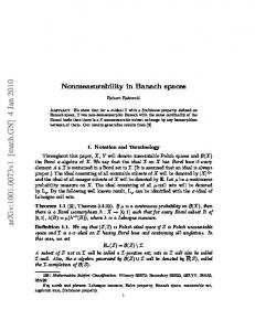
To see first that the intersection of finitely many prox-regular sets may not be prox-regular, consider the example in R2 with its euclidian norm illustrated by the figure on the right, where the set C1 is the whole line (x1 x2 ), (xi )i being a sequence of points on C1 that converges to some x ∈ C1 , and the set C2 is the hatched _ surface delimited on one side by the closed arc x1 x of the half circle with radius R = kx1 − xk/2 and on its other side by the _ arcs of the circles (all with the same radius r < R) xi xi+1 , i ∈ N, so that x belongs also to C2 . It is easily seen that while C1 and C2 are both prox-regular at x (they are even uniformly prox-regular), their intersection C1 ∩ C2 is not prox-regular at the point x. To provide general sufficient conditions under which the prox-regularity of intersection or inverse image is preserved, we Fig.1. Intersection of need first to recall the concept of calmness. Translating the prox-regular sets concept of calmness of a multivalued mapping in [40] we say m that the intersection of a finite family of sets (Ck )m k=1 is metrically calm at a point x ∈ ∩ Ck provided there exist a constant γ > 0 and a neighbourhood U of x such that m

d(x, ∩ Ck ) ≤ γ ( d(x, C1 ) + · · · + d(x, Cm )) k=1

for all x ∈ U.

k=1

(7.1)

Let now F : X → Y be a mapping from X into another uniformly convex Banach space Y and let D be a subset of Y and x ∈ F −1 (D). As above we say that the mapping F is metrically calm at x relatively to the set D when there exist a constant γ > 0 and a neighbourhood U of x such that d(x, F −1 (D)) ≤ γd(F (x), D) for all x ∈ U.

(7.2)

Proposition 7.1 Let (Ck )m k=1 be a finite family of closed sets of X and let D be a closed set of Y . (a) If all sets Ck are N P -hyporegular at a point x of all the sets Ck and if the intersection is m metrically calm at x, then this intersection set ∩ Ck is N P -hyporegular at x too. k=1

(b) If a mapping F : X → Y is of class C 1,1 around a point x ∈ F −1 (D) and metrically calm at x relatively to D and if D is N P -hyporegular at F (x), then the set F −1 (D) is N P hyporegular at x. m

Proof: Assume that each set Ck is N P -hyporegular at x and put C := ∩ Ck . By definition k=1

of N P -hyporegularity (see 5.1) it is easily seen that there exist some real number r > 0 and some open neighbourhood U of x such that for each k = 1, . . . , m we have for all x ∈ Ck ∩ U and u∗ ∈ NCPk (x) ∩ B∗ hu∗ , x0 − xi ≤ (2r)−1 kx0 − xk2 28

for all x0 ∈ Ck ∩ U.

(7.3)

Restricting the neighbourhood U if necessary, we may suppose that the inequality (7.1) holds upon U . Fix any x ∈ C ∩ U and take any x∗ ∈ NCP (x) with kx∗ k ≤ 1. We have that x∗ ∈ NCF (x) and hence x∗ ∈ ∂F dC (x) since one knows that ∂F dC (x) = NCF (x) ∩ B∗ (see, e.g., [35, Corollary 1.96]). This inequality (7.1) and the definition of Fréchet subgradient easily yields that x∗ ∈ γ∂F (dC1 +· · ·+dCm )(x) and hence in particular x∗ ∈ γ∂L (dC1 +· · ·+dCm )(x). The functions dCk being Lipschitzian, the formula of the Mordukhovich subdifferential of a finite sum of locally Lipschitzian functions (see, e.g., [35, Theorem 3.36]) ensures us that there exist u∗k ∈ ∂L dCk (x) such that γ −1 x∗ = u∗1 + · · · + u∗m . Restricting again the neighbouhood U , by Theorem 3.2 we have u∗k ∈ ∂P dCk (x) = NCP (x) ∩ B∗ which by (7.3) gives hu∗k , x0 − xi ≤ (2r)−1 kx0 − xk2 for every x0 ∈ Ck ∩ U . Consequently for any x0 ∈ C ∩ U we obtain hγ −1 x∗ , x0 − xi ≤ m(2r)−1 kx0 − xk2 and this obviously implies that the intersection set C is N P -hyporegular at x, that is, (a) is proven. Let us now establish (b). Fix some open convex neighbourhood U of x over which (7.2) holds and over which the mapping F as well as its derivative DF (·) are Lipschitzian with Lipschitzian constants K and K1 respectively. For S := F −1 (D) fix any x ∈ U ∩ S and x∗ ∈ NSP (x) with kx∗ k ≤ 1. As above we have x∗ ∈ ∂F dS (x) and this entails by (7.2) that x∗ ∈ γ∂F (dD ◦ F )(x) and hence x∗ ∈ γ∂L (dD ◦ F )(x). The subdifferential chain rule (see, e.g., [35, Corollary 3.43]) gives some y ∗ ∈ ∂L dD (F (x)) such that γ −1 x∗ = y ∗ ◦ DF (x). Fix by (5.1) some open neighbourhood V of F (x) and some constant r > 0 such that hv ∗ , y 0 − yi ≤ (2r)−1 ky 0 − yk2

for all y ∈ V ∩ D, y 0 ∈ V ∩ D and v ∗ ∈ NDP (y) ∩ B∗ , (7.4)

and such that the equality concerning the subdifferentials of the distance function in Theorem 3.2 holds with dD at all points of V ∩ D. Restricting the open convex neighbourhood U of x if necessary, we may suppose that F (U ) ⊂ V and that ∂L dD (F (u)) = ∂P dD (F (u)) for all u ∈ U ∩ S according to Theorem 3.2. Then (7.4) yields hy ∗ , y 0 − F (x)i ≤ (2r)−1 ky 0 − F (x)k2

for all y 0 ∈ V ∩ D.

(7.5)

Fix any x0 ∈ S ∩ U and write Z 0

1

0

F (x ) − F (x) = DF (x)(x − x) +

(DF (x + t(x0 − x)) − DF (x)) (x0 − x) dt

0

and then hγ

−1 ∗

Z 0

∗

1

0

x , x − xi = hy , F (x ) − F (x)i −

hy ∗ ◦ (DF (x + t(x0 − x)) − DF (x)) , x0 − xi dt.

0

Using (7.5) we obtain hx∗ , x0 − xi ≤ γ(2r)−1 kF (x0 ) − F (x)k2 + γK1 kx0 − xk2 ≤ γ(K 2 (2r)−1 + K1 )kx0 − xk2 . The latter being true for all x, x0 ∈ S ∩ U and x∗ ∈ NSP (x) ∩ B∗ , we conclude that the set S ¥ is N P -hyporegular at x.

29

For the convenience of the reader we made the choice to prove first the N P -hyporegularity of the intersection and then to give the additional arguments yielding to the N P -hyporegularity of the inverse image. However the case of the intersection can be derived from that of the inverse image. Indeed putting Y = X m , F (x) = (x, . . . , x) for all x ∈ X, and m D = C1 × · · · × Cm we see that F −1 (D) = ∩ Ck and then some direct arguments and k=1

computation allow us to obtain through (b) the result of (a). We state now the following corollary which is a direct consequence of Corollary 5.1. Corollary 7.2 Assume that the moduli of convexity and smoothness of the norm of X are of power type and the power type of convexity is q = 2. Then under the assumptions of m Proposition 7.1 the sets ∩ Ck and F −1 (D) are prox-regular at x. k=1

When the spaces (X, k · k) and (Y, k · k) are Hilbert spaces, Proposition 7.1 translates, according to Corollary 5.1 and Proposition 5.2, the preservation of prox-regularity. Corollary 7.3 Assume that X and Y are Hilbert spaces for their respective norms. Let (Ck )m k=1 be a finite family of closed sets of X and let D be a closed set of Y . (a) If all sets Ck are prox-regular at a point x of all the sets Ck and if the intersection is m metrically calm at x, then this intersection set ∩ Ck is prox-regular at the point x. k=1

(b) If a mapping F : X → Y is of class C 1,1 around a point x ∈ F −1 (D) and metrically calm at x relatively to D and if D is prox-regular at F (x), then the set F −1 (D) is prox-regular at x. An analysis of the proof of Proposition 7.1 reveals that a uniform version also holds. We state it only in the case of an intersection and let the case of the inverse image to the reader. Proposition 7.4 Assume that all the closed sets Ck , k = 1, . . . , m, are r-uniformly N P hyporegular (resp. r-uniformly prox-regular and (X, k · k) is a Hilbert space) and that their intersection is calm at anyone of its points with the same modulus γ of metric calmness m in (7.1). Then the set ∩ Ck is r0 -uniformly N P -hyporegular (resp. r0 -uniformly metrically k=1

prox-regular) with r0 := r/(mγ). In the literature there are conditions with normal cones easy to handle ensuring the metric calmness inequalities (7.1) and (7.2). For example such a condition for (7.1) is known (see, e.g., [28, p. 548-549]) under the name of general position condition for intersection of finitely many sets. In the context of our uniformly convex Banach space, the concept can be translated by saying that the closed sets C1 , . . . , Cm are (relative to the Fréchet m normal cone) in sequential general position at x ∈ ∩ Ck whenever for any sequence of k=1

tuples (x1,n , · · · , xm,n , x∗1,n , · · · , x∗m,n )n such that xk,n ∈ Ck , xk,n → x, x∗k,n ∈ NCFk (xk,n ) ∩ B∗ m P and such that k x∗k,n k → 0, one has kx∗k,n k → 0 for any k = 1, . . . , m. k=1

30

Another condition which is much easier to handle involves as above a property with normal cones but at the fixed point x. It probably appears for the first time as one of the assumptions of Theorem 4.10 of Federer’s seminal paper [26] for sets of Rn which are not submanifolds. The sets Ck , k = 1, . . . , m, are (relative to the limiting normal cone) in pointbased general position at x provided the equality x∗1 + · · · + x∗m = 0 with x∗k ∈ NCLk (xk ) entails x∗1 = · · · = x∗m = 0. Recall now that a closed set of X is compactly epi-Lipschitzian at x ∈ C (a concept due to J. M. Borwein and H. M. Strójwas [11]) if there exist a compact set Q, a neighbourhood V of zero, a neighbourhood U of x in X, and a positive real number ε such that C ∩ U + tV ⊂ C + tQ for all t ∈]0, ε]. Of course any closed subset of X is compactly epi-Lipschitzian at any of its points whenever the space X is finite dimensional. m

Corollary 7.5 Let (Ck )m k=1 be a finite family of closed sets of X and x ∈ ∩ Ck . Then the k=1

following hold. (a) If the sets Ck are in sequential general position at x and if each set Ck is N P -hyporegular m at x (resp. prox-regular at x and (X, k · k) is a Hilbert space), then the intersection ∩ Ck is k=1

N p -hyporegular (resp. prox-regular) at x. (b) If all the sets Ck except at most one are compactly epi-Lipschitzian at x, then the sequential general position in (a) may be replaced by the corresponding pointbased general position at x. (c) If the space X is finite dimensional, again the sequential general position in (a) may be replaced by the corresponding pointbased general position at x. Proof: (a) Since the uniformly convex Banach space X is an Asplund space, the sequential general position is known to entail the metric calmness property (7.1) (and even more) according to Proposition 6 in p. 548 and Theorem 2 in p. 545 of [27] (for example). Then the conclusion of (a) follows from Proposition 7.1 (resp. Corollary 7.3). (b) The result comes from the fact that the assumption of compactly epi-Lipschitzian property combined with the pointbased general position at x ensures (see, e.g., [30, Theorem 3.4]) that the intersection is metrically regular and hence metrically calm at x. (c) This is a direct consequence of (b). ¥ The result in (c) was previously established in (5) of Theorem 4.10 in [26].

8

Conical derivative of the mapping PC

The following result is well-known for convex sets of Hilbert space (see Zarantonello [46, p. 300]). The term conical derivative has been coined in page 301 of [46]. The result has been independently extended by Canino [15] to closed p-convex sets of Hilbert space and by Shapiro [41] to closed sets with 2-order tangential property of Hilbert space too. It is 31

actually known (see [39]) that, in the context of Hilbert space, the concept of p-convex set is equivalent to uniform prox-regularity and the 2-order tangential property is equivalent to the local prox-regularity. The related result in [41] may then be translated for prox-regular sets. Note also that the proof in [15] still holds for sets which are prox-regular at the considered point of the Hilbert space. Our proposition below deals with the context of uniformly convex space. Proposition 8.1 Assume that the moduli of uniform convexity and smoothness of the norm k · k of X are of power type. Assume also that the closed set C of X is prox-regular at x ∈ C. Then there exists an open neighbourhood U of x such that PC is single valued and continuous 1 on U and such that for any x ∈ U ∩C and y ∈ X for which the mapping t 7→ [PC (x+ty)−x] t is bounded on some interval ]0, t0 ], one has 1 lim [PC (x + ty) − x] = PKC (x) (y) t↓0 t 1 and the directional derivative d0C (x; y) := lim [dC (x + ty) − dC (x)] of dC at x in the direction t↓0 t y exists and d0C (x; y) = d(y, KC (x)), which translates in the terminology of [46] that d0C (x; ·) is a conical derivative. Proof: By the inequality (3.12) of the proof of Theorem 3.2, there exist ε, r > 0 with ε < 1/2 such that PC is a single-valued continuous mapping on B(x, ε) and 2 hx∗ − u∗ , u − xi ≤ kx − uk ωr+1 (kx − uk) r

(8.1)

for all x, u ∈ B(x, ε) and all x∗ ∈ NCP (x), u∗ ∈ NCP (u) with kx∗ k ≤ 1 and ku∗ k ≤ 1, where ωr+1 is the modulus of uniform continuity of the duality mapping J over the bounded set 1 (r +1)B. Let x ∈ B(x, ε)∩C, y ∈ X, and t0 > 0 such that the mapping t 7→ [PC (x+ty)−x] t is bounded on ]0, t0 ], say by β > 0. We may suppose that for all t ∈]0, t0 ] we have x + ty ∈ 1 B(x, ε) and PC (x + ty) ∈ B(x, ε). For any t ∈]0, t0 ] putting h0t := [PC (x + ty) − x], we see t that 1 y − h0t = [x + ty − PC (x + ty)] t 0 and hence y − ht ∈ P NC (PC (x + ty)), i.e., J(y − h0t ) ∈ NCP (PC (x + ty)). Take now any sequence (tn )n of ]0, t0 ] converging to 0. The sequence (J(y − h0tn ))n being bounded, there exists an increasing function σ : N → N such that the sequence (J(y − h0tσ(n) ))n converges weakly star to J(y − h) for some vector h ∈ X. As NCP (x) = NCL (x) (see Theorem 3.2), we have J(y − h) ∈ NCP (x). Put hn := h0tσ(n) . By (8.1) there exists some constant γ > 0 independent of n such that for λn := tσ(n) hJ(y − hn ) − J(y − h), x − PC (x + λn y)i ≤

γ kPC (x + λn y) − xk ωr+1 (kPC (x + λn y) − xk). r 32

The latter inequality is equivalent to hJ(y − hn ) − J(y − h), −λn hn i ≤

γ kPC (x + λn y) − xk ωr+1 (kPC (x + λn y) − xk), r

that is, hJ(y − hn ) − J(y − h), (y − hn ) − (y − h)i − hJ(y − hn ) − J(y − h), hi γ 1 ≤ k [PC (x + λn y) − x]k ωr+1 (kPC (x + λn y) − xk). r λn If max{ky − hn k, ky − hk} = 0 for infinitely many n, then for all these integers n we have y = hn = h and hence by definition of hn we obtain h = λ1n [PC (x + λn y) − x], which yields h ∈ KC (x). Suppose now that max{ky − hn k, ky − hk} > 0 for all n not less than some n0 . According to (2.2) for some constant K2 > 0 we have for all n ≥ n0 µ ¶ khn − hk 2 K2 (max{ky − hn k, ky − hk}) δk·k 2(max{ky − hn k, ky − hk}) γ 1 ≤ hJ(y − hn ) − J(y − h), hi + k [PC (x + λn y) − x]k ωr+1 (kPC (x + λn y) − xk), r λn and since the first expression of the second member tends to 0 and the modulus of convexity δk·k is an increasing function with δk·k (t) −→ 0, it is not difficult to see that khn − hk → 0 t↓0

and by definition of hn we obtain h ∈ KC (x). So in any case, we have h ∈ KC (x) and the sequence (hn )n strongly converges to h. Take now any v ∈ KC (x). Since KC (x) = TC (x) according to Theorem 3.2, there is a sequence (zn )n converging to v such that x + λn zn ∈ C for all n. This entails that for all n kx + λn y − (x + λn zn )k ≥ kx + λn y − PC (x + λn y)k, which is equivalent to ky − zn k ≥ ky +

1 [x − PC (x + λn y)]k. λn

Then passing to the limit with n → ∞, we obtain ky − vk ≥ ky − hk for all v ∈ KC (x), which means that h = PKC (x) (y). So for any sequence of positive numbers (tn )n converging to 0 there exists a subsequence (tσ(n) )n such that lim

1

n→∞ tσ(n)

[PC (x + tσ(n) y) − x] = PKC (x) (y).

Consequently

1 lim [PC (x + ty) − x] = PKC (x) (y). (8.2) t↓0 t Concerning the equality of the directional derivative of the distance function to the set C, observe first that for any positive number t small enough 1 1 [dC (x + ty) − dC (x)] = dC (x + ty) = 1t kPC (x + ty) − (x + ty)k t t = k 1t [PC (x + ty) − x] − yk. 33

Then taking (8.2) into account and passing to the limit when t ↓ 0 give that the directional derivative d0C (x; y exists and d0C (x; y) = kPKC (x) (y) − yk = d(y, KC (x)). ¥ In the case of a Hilbert space X the mapping PC is Lipschitzian near x (see [39]) and hence the boundedness assumption of the proposition above is fulfilled and one recovers in Corollary 8.2 below the result of Proposition 2.12 in [15] and Theorem 3.1 in [41]. The result is proved in [41] through some properties of solutions of perturbed optimization problems satisfying some appropriate conditions. The proof in [15] is based on the duality in Hilbert space between the tangent cone KC (x) and the primal normal cone P NC (x) for prox-regular sets C. Such a duality property is not available in the non Hilbert setting because of the nonlinearity of the duality mapping J. Instead, our proof of Proposition 8.1 above is related to the tangential regularity of C established in Theorem 3.2 and to the sequential characterization of the Clarke tangent cone (recalled in the beginning of Section 3). Corollary 8.2 ([15, Proposition 2.12] and [41, Theorem 3.1]) Assume that X is a Hilbert space and that C is prox-regular at x ∈ C. Then for some neighbourhood U of x one has for all x ∈ U ∩ C and y ∈ X the directional derivatives of PC and dC at x in the direction y exist and 1 lim [PC (x + ty) − x] = PKC (x) (y) and d0C (x; y) = d(y, KC (x)). t↓0 t

9

Convergence

In this section we are interested in the behaviour of the projection mapping under convergence of prox-regular sets. Let us begin by recalling some properties of the projection mapping of a prox-regular set and by providing some additional facts. Consider a uniformly r-prox-regular closed set C. We saw in the statement of Theorem 2.6 that the function d2C is Fréchet differentiable on the r-open neighborhood OC (r) and that PC is a single-valued and norm-to-norm continuous mapping from OC (r) into C. Moreover, Proposition 5.5 in [9] gives for any x ∈ OC (r) 1 D( d2C )(x) = J(x − PC (x)). 2

(9.1)

Concerning the continuity of PC , Theorem 5.2 in [9] says more, in the sense that PC is locally Hölder continuous on OC (r). The following two propositions furnish some further points that we will need in Theorem 9.4 below. Recall that q (resp. s) denotes the power type of the modulus of convexity (resp. smoothness) of the norm of X. Proposition 9.1 Assume that the moduli of uniform convexity and smoothness of the norm k · k of X are of power type q and s respectively. Let r, r0 be two positive numbers with r0 < 2r

34

and let a number ρ > 0. Then there exists some constant γ ≥ 0 depending only on r, r0 and ρ such that, for any uniformly r-prox-regular closed subset C of X, one has 1

kPC (x1 ) − PC (x2 )k ≤ γkx1 − x2 k q and |Dd2C (x1 ) − Dd2C (x2 )| ≤ γkx1 − x2 k

s−1 q

(9.2)

for all x1 , x2 ∈ OC (r0 ) ∩ ρB. Proof: Take α ∈]0, 1/2[ such that r0 = αr. By Step 1 of the proof of Theorem 5.2 in [9] P the truncated normal cone set-valued mapping NC,r (·) is J-hypomonotone of degree 1 and P (·). Referring to the proof of Lemma 2.7 in [9] with hence so is the set-valued mapping NC,αr P T (·) := NC,αr (·) and r := 1, since α−1 > 2r the development there reveals that, fixing λ satisfying 2α < λ < 1, there exists some constant γ 0 > 0 depending only on α, ρ, and r such P −1 ) is on ρB ∩ Dom Q a single valued mapping for which that Q := (I + αJ ∗ ◦ NC,r 1

kQ(x1 ) − Q(x2 )k ≤ γ 0 kx1 − x2 k q

for all x1 , x2 ∈ ρB ∩ Dom Q.

(9.3)

Observe now that for x ∈ OC (αr) we have J(x − PC (x)) ∈ NCP (PC (x)) (by definition of proximal normal functional) and kJ(x − PC (x))k < αr and that those two facts imply P P −1 J(x − PC (x)) ∈ αNC,r (PC (x)), that is, PC (x) = (I + αJ ∗ ◦ NC,r ) (x). We may then reformulate (9.3) in the form 1

for all x1 , x2 ∈ OC (r0 ) ∩ ρB.

kPC (x1 ) − PC (x2 )k ≤ γ 0 kx1 − x2 k q

Concerning the square distance function d2C , we know that it is (see 9.1 ) Fréchet differentiable on OC (r) with Dd2C (x) = 2J(x − PC (x)) for all x ∈ OC (r). So using (2.9) and the latter inequality above, we have for all x1 , x2 ∈ OC (r0 ) ∩ ρB kDd2C (x1 ) − Dd2C (x2 )k ≤ 2Lρ kx1 − PC (x1 ) − x2 + PC (x2 )ks−1 1 ≤ 2Lρ (kx1 − x2 k + γ 0 kx1 − x2 k q )s−1 s−1 1 ≤ 2Lρ (γ 0 + kx1 − x2 k1− q )s−1 kx1 − x2 k q s−1 1 ≤ 2Lρ (γ 0 + (2ρ)1− q )s−1 kx1 − x2 k q . 1

It suffices to take γ = max{γ 0 , 2Lρ (γ 0 + (2ρ)1− q )s−1 } to obtain both inequalities in the statement of the proposition. ¥ In the proposition above, under the restriction r0 < r/2, the power of Hölder continuity of PC over OC (r0 )∩ρB is the constant 1/q (the inverse of the power type of uniform convexity of k · k), i.e., only the modulus γ of Hölder continuity varies with r0 and ρ. Relaxing the restriction r0 < r/2 into r0 < r and letting the power of Hölder continuity depending also on r0 and ρ, we can prove the following result of Hölder continuity of PC on OC (r0 ) ∩ ρB but this time with any r0 < r. Before stating the result, recall that for any r > 0 the (closed) r-enlargement C(r) of C is given by C(r) := {x ∈ X : d(x, C) ≤ r}. Proposition 9.2 Assume that the moduli of uniform convexity and smoothness of the norm k · k of X are of power type q and s respectively. Let ρ, r, r0 be positive real numbers with 35

r0 < r. Then there exist some positive constants γ and θ ≤ 1 both depending only on r0 , r and ρ, such that for any uniformly r-prox-regular closed set C of X one has kPC (x1 ) − PC (x2 )k ≤ γkx1 − x2 kθ and |Dd2C (x1 ) − Dd2C (x2 )| ≤ γkx1 − x2 kθ(s−1)

(9.4)

for all x1 , x2 ∈ OC (r0 ) ∩ ρB. n More precisely, defining (αn )n by α1 = 12 and αn+1 = 1+α , then for any n ∈ N, ρ > 0, 2 0 α ∈]0, αn [, there exists some positive real number k (depending only on ρ, α0 and n) such that, for any uniformly r-prox-regular closed set C of X, the metric projection mapping PC is H¨ older continuous on OC (α0 r) ∩ ρB with power θ := q1n and with modulus k. Proof: Let us call P(n) the property above in the second part of the proposition for PC of any uniformly r-prox-regular closed set C. Note that P(1) is Proposition 9.1. Suppose that P(n) is fulfilled, and fix any uniformly r-prox regular closed set C and any ρ > 0, α0 ∈]0, αn [. We may suppose that OC (r) ∩ ρB 6= ∅. By Theorem 2.6 and Lemma 5.4 in [9], the closed set C(α0 r) is uniformly (1 − α0 )r-prox-regular. Then applying now Proposition 9.1 to the set C(α0 r) yields that for any λ ∈]0, 1[, PC(α0 r) is Hölder continuous on OC(α0 r) (λ

1 − α0 r) ∩ ρB with power 1/q 2

(9.5)

and with modulus depending only on ρ, λ, α0 , and r. On the other hand, we have that for any t > 0, OC (α0 r + t) = OC(α0 r) (t). Indeed, from Lemma 5.3 (a) in [9] (see also [14]), for any τ > 0 and any u ∈ / C(τ ) one has dC (u) = τ + dC(τ ) (u). Hence, for any u ∈ X, one has the equivalence dC (u) < α0 r + t ⇔ dC(α0 r) (u) < t, that is, the desired equality holds. This entails that 1 − α0 1 − α0 OC(α0 r) (λ r) = OC (α0 r + λ r). (9.6) 2 2 By (9.5) and (9.6) there exists some constant K1 > 0 (depending only on ρ, λ, α0 , and r) such that kPC(α0 r) (u1 ) − PC(α0 r) (u2 )k ≤ K1 ku1 − u2 k1/q for all ui ∈ OC (α0 r + λ

1 − α0 r). 2

(9.7)

Fixing bρ ∈ OC (r) ∩ ρB 6= ∅, we find some aρ ∈ C with kaρ k ≤ r + ρ. Combining this with (9.7), we obtain that there is some ρ0 > 0 (depending only on ρ, λ, α0 , and r) such that kPC(α0 r) (u)k ≤ ρ0

for all u ∈ (ρB) ∩ OC (α0 r + λ

1 − α0 r) 2

(9.8)

(take u1 = u and u2 = aρ in (9.7)). The equality (9.6) also implies, according to Theorem 0 r) \ C(α0 r), the points y := PC(α0 r) (u) and z := PC (y) 2.6 that for any u ∈ OC (α0 r + λ 1−α 2 exist. By (c) of Lemma 5.3 in [9], for any such u we have consequently z = PC (u) and so, 0 PC (u) = PC ◦ PC(α0 r) (u). From this, if u1 , u2 ∈ (ρB) ∩ (OC (α0 r + λ 1−α r) \ C(α0 r)), then for 2 00 0 any α ∈]α , αn [ we have kPC (u1 ) − PC (u2 )k = kPC (PC(α0 r) (u1 )) − PC (PC(α0 r) (u2 ))k ≤ K2 kPC(α0 r) (u1 ) − PC(α0 r) (u2 )k1/q 36

n

for some constant K2 > 0 (depending only on ρ0 , α00 , and n), according to P(n) and to the fact that, by (9.8), for i = 1, 2, PC(α0 r) (ui ) ∈ ρ0 B ∩ OC (α00 r). Taking (9.7) into account we obtain that there exists some constant K3 (depending only on ρ, λ, α0 , r and n) such that 0 for all u1 , u2 ∈ (ρB) ∩ (OC (α0 r + λ 1−α r) \ C(α0 r)) 2 kPC (u1 ) − PC (u2 )k ≤ K3 ku1 − u2 k1/q

n+1

(9.9) 0

and this inequality is still true for all ui ∈ ρB satisfying α0 r ≤ d(ui , C) < α0 r + λ 1−α r. On 2 ρB ∩ C(α0 r), P(n) ensures that PC also has the Hölder continuity property with power 1/q n and hence also with power 1/q n+1 (because of the boundedness of ρB ∩ C(α0 r)). Then there exists some positive constant K4 (depending only on ρ, λ, α0 , r and n) such that kPC (u1 ) − PC (u2 )k ≤ (K4 /2)ku1 − u2 k1/q

n+1

0

r) satisfying either d(ui , C) ≥ α0 r for i = 1 and for all u1 , u2 ∈ (ρB) ∩ (OC (α0 r + λ 1−α 2 i = 2 or d(ui , C) ≤ α0 r for i = 1 and i = 2. In the remaining case where u1 , u2 ∈ 0 (ρB) ∩ (OC (α0 r + λ 1−α r) with d(u1 , C) < α0 r and d(u2 , C) > α0 r, the continuity of d(·, C) 2 over the line segment [u1 , u2 ] yields some point u0 ∈]u1 , u2 [ such that d(u0 , C) = α0 r; then kPC (u1 ) − PC (u2 )k ≤ (K4 /2)(ku1 − u0 k1/q

n+1

+ ku0 − u2 k1/q

n+1

) ≤ K4 (ku1 − u2 k1/q

n+1

,

the second inequality being due to the inequalities kui − u0 k ≤ ku1 − u2 k. The mapping PC 0r is then Hölder continuous on ρB ∩ (OC (α0 r + λ 1−α r)) with modulus K4 and power 1/q n+1 . 2 We have shown that, for any λ ∈]0, 1[, α0 ∈]0, αn [, and ρ > 0, there exists some positive real number k (depending only on ρ, α0 , λ, and n) such that, for any uniformly r-prox-regular 0 set C, the metric projection mapping PC is Hölder continuous on ρB ∩ OC (α0 r + λ 1−α r) 2 n+1 0 with power 1/q and with modulus k. This means that for any α ∈]0, αn [ there is some positive k (depending only on ρ, α0 , and n) such that, for any uniformly r-prox-regular set 0 C of X, the mapping PC is Hölder continuous on ρB ∩ OC (α0 r + 1−α r) with power 1/q n+1 2 0 0 and modulus k. Consequently P(n + 1) holds true since α0 r + 1−α r = 1+α r. 2 2 2 The Hölder continuity of the function DdC (·) is obtained like in the proof of Proposition 9.1. ¥ Remark 9.3 When (X, k · k) is a Hilbert space, where k · k is the norm associated with the inner product, the behaviour of PC (·) and Dd2C (·) is distinctly better. Indeed, by [39] for any real positive numbers r, r0 with r0 < r and any uniformly r-prox-regular closed set C of X one has r kx1 − x2 k kPC (x1 ) − PC (x2 )k ≤ r − r0 for all x1 , x2 ∈ OC (r0 ), and hence kDd2C (x1 ) − Dd2C (x2 )k ≤ 2(1 +

r )kx1 − x2 k r − r0

according to (9.1) and to the Lipschitz property of J here with Lipschitz modulus 1. So, not only the Lipschitz continuity (instead of the Hölder one) is available for the metric projection but also no restriction to bounded subsets of OC (r0 ) is required. 37

We can now study convergence properties of families of uniformly prox-regular sets. Let T ∪ {t0 } be a topological space with t0 as a cluster point of T . Recall that a family (Ct )t∈T of non empty closed subsets of X converges in the sense of Attouch-Wets (see [1, 4, 40]) to a closed subset C of X when t goes to t0 provided for each positive real number ρ one has sup |dCt (x) − dC (x)| −→ 0.

(9.10)

t→t0

x∈ρB

Theorem 9.4 Assume that the moduli of uniform convexity and smoothness of the norm k · k of X are of power type. Let (Ct )t∈T be a family of closed uniformly r-prox-regular sets of X which converges in the sense of Attouch-Wets to a closed set C of X. Then C is uniformly r-prox-regular and for each x0 ∈ X satisfying d(x0 , C) < r the mapping t 7→ PCt (x0 ) and the function t 7→ Dd2Ct (x0 ) are defined on a neighbourhood of t0 and PCt (x0 ) −→ PC (x0 ) t→t0

and Dd2Ct (x0 ) −→ Dd2C (x0 ).

(9.11)

t→t0

Proof: Fix a positive number r0 with d(x0 , C) < r0 < r and choose by (9.10) some neighbourhood T00 of t0 and some β > 0 such that d(x, Ct ) < r0 for all t ∈ T00 \ {t0 } and x ∈ x0 + 2βB. According to Proposition 9.2, there exist some positive constants γ and σ ≤ 1 (both depending only x0 , β, r0 and r) such that for all t ∈ T00 with t 6= t0 and x1 , x2 ∈ x0 +2ρB the derivatives Dd2Ct (xi ), i = 1, 2, exist and kDd2Ct (x1 ) − Dd2Ct (x2 )k ≤ γkx1 − x2 kσ . 00

(9.12)

00

Fix another neighbourhood T0 of t0 with T0 ⊂ T00 and such that, according to (9.10), the function v given for ρ := 1 + 2β + kx0 k by v(t) := sup |dCt (x) − dC (x)| x∈ρB

00

is bounded on T0 := T0 \ {t0 }. Writing dCt (x) ≤ dCt (x0 ) + kx − x0 k ≤ dC (x0 ) + kx − x0 k + v(t) for all x ∈ X and t ∈ T, we see that there exists some constant M > 0 such that dCt (x) ≤ M/2 for all (t, x) ∈ T0 × ρB.

(9.13) 00

Fix now any positive number ε < β. Choose by (9.10) a neighbourhood T 0 ε ⊂ T0 of t0 such that for Tε := T 0 ε \ {t0 } |dCt (x) − dC (x)| ≤

εσ+1 2

for all t ∈ Tε and x ∈ ρB.

Fix any x ∈ B(x0 , β), any w ∈ X with kwk = ε, and any t, τ ∈ Tε . We have Z 1 2 2 2 hDd2Ct (x + sw) − Dd2Ct (x), wi ds dCt (x + w) − dC (x) = hDdCt (x), wi + 0

38

(9.14)

and a similar equality with d2Cτ in place of d2Ct , hence hDd2Ct (x) − Dd2Cτ (x), wi = [d2Ct (x + w) − d2Cτ (x + w)] − [d2Ct (x) − d2Cτ (x)] Z 1 Z 1 2 2 hDd2Cτ (x + sw) − Dd2Cτ (x), wi. − hDdCt (x + sw) − DCt (x), wi + 0

0

Further, on the one hand by (9.12) we have ¯Z 1 ¯ Z ¯ ¯ ¯ hDd2C (x + sw) − Dd2C (x), wi ds¯ ≤ t t ¯ ¯ 0

1

γsσ kwkσ+1 ds =

0

1 γkwkσ+1 ≤ γεσ+1 σ+1

and a similar inequality with d2Cτ in place of d2Ct . On the other hand by (9.13) and (9.14), with y := x + w or y := x we also have |d2Ct (y) − d2Cτ (y)| = (dCt (y) + dCτ (y))|dCt (y) − dCτ (y)| ≤ M εσ+1 . Consequently hDd2Ct (x) − Dd2Cτ (x), wi ≤ (2M + 2γ)εσ+1 and hence that for every u in X with kuk = 1 hDd2Ct (x) − Dd2Cτ (x), ui ≤ (2M + 2γ)εσ , which ensures that kDd2Ct (x) − Dd2Cτ (x)k ≤ (2M + 2γ)εσ . This uniform Cauchy property says that the family (Dd2Ct )t converges uniformly to some mapping from B(x0 , β) into X ∗ . This is known to entail that the function d2C is Fréchet differentiable on B(x0 , β) and hence, in particular, Fréchet differentiable at x0 with Dd2Ct (x0 ) −→ Dd2C (x0 ). t→t0

(9.15)

Then the function dC is Fréchet differentiable on the open tube UC (r) and this differentiability property translates through Theorem 2.6 the uniform r-prox-regularity of C. Further (9.1) and (9.15) yield PCt (x0 ) −→ PC (x0 ). t→t0

This completes the proof of the proposition.

¥

References [1] H. Attouch and R. J.-B. Wets, Isometries for the Legendre-Fenchel transform, Trans. Amer. Math. Soc. 296 (1986), 33-60. [2] D. Aussel, A. Daniilidis and L. Thibault, Subsmooth sets: Functional characterizations and related concepts, Trans. Amer. Math. Soc. 357 (2004), 1275-1301. 39

[3] B. Beauzamy, Introduction to Banach spaces and their geometry, 2nd edition, NorthHolland, Amsterdam (1985). [4] G. Beer, Topologies on Closed and Closed Convex Sets, Kluwer Academic Publishers, North-Holland, Dordrecht (1993). [5] F. Bernard and L. Thibault, Prox-regular functions in Hilbert spaces, J. Math. Anal. Appl. 303 (2005), 1–14. [6] F. Bernard and L. Thibault, Prox-regular functions and sets in Banach spaces, SetValued Analysis 12 (2004), 25–47. [7] F. Bernard and L. Thibault, Uniform prox-regularity of functions and epigraphs in Hilbert spaces, Nonlinear Anal. 60 (2005), 187-207. [8] F. Bernard, L. Thibault and D. Zagrodny, Integration of primal lower nice functions in Hilbert spaces, J. Optimization Theory Appl. 124 (2005), 561-579. [9] F. Bernard, L. Thibault and N. Zlateva, Characterizations of prox-regular sets in uniformly convex Banach spaces, J. Convex Analysis 13 (2006), 525-559. [10] J. M. Borwein and J. R. Giles, The proximal normal formula in Banach space, Trans. Amer. Math. Soc. 302 (1987), 371–381. [11] J. M. Borwein and H. M. Strójwas, Tangential approximations, Nonlinear Anal. 9 (1985), 1347-1366. [12] J. M. Borwein and H. M. Strójwas, Proximal analysis and boundaries of closed sets in Banach space. I. Theory, Canad. J. Math. 38 (1986), 431–452. [13] J. M. Borwein and H. M. Strójwas, Proximal analysis and boundaries of closed sets in Banach space. II. Applications, Canad. J. Math. 39 (1987), no. 2, 428–472. [14] M. Bounkhel and L. Thibault, On various notions of regularity of sets in nonsmooth analysis, Nonlinear Anal. 48 (2002), 223–246. [15] A. Canino, On p-convex sets and geodesics, J. Differential Equations 75 (1988), 118–157. [16] F. H. Clarke, Optimization and nonsmooth analysis, John Wiley & Sons, New York (1983). [17] F. H. Clarke, Yu. S. Ledyaev, J. R. Stern and R. P. Wolenski, Nonsmooth Analysis and Control Theory, Springer, New York (1998). [18] F. H. Clarke, J. R. Stern and R. P. Wolenski, Proximal smoothness and the lower-C2 property, J. Convex Analysis 2 (1995), 117–144. [19] G. Colombo and V. V. Goncharov, Variational inequalities and regularity properties of sets in Hilbert spaces, J. Convex Analysis 8 (2001), 197–221. 40

[20] R. Correa, A. Jofre and L.Thibault, Subdifferential monotonicity as characterization of convex functions, Numer. Funct. Anal. Optimiz. 15 (1994), 531–536. [21] M. Degiovanni, A. Marino and M. Tosques, General properties of (p, q)-convex functions and operators, Ricerche Mat. 32 (1983), 285–319. [22] R. Deville, G. Godefroy and V. Zizler, Smoothness and Renormings in Banach Spaces, Pitman Monographs and Surveys in Pure and Applied Mathematics, 64, John Wiley & Sons Inc., New York (1993). [23] J. Diestel, Geometry of Banach spaces – selected topics. Lecture Notes in Mathematics, vol. 485, Springer-Verlag, Berlin-New York (1975). [24] J. F. Edmond and L. Thibault, BV solutions of nonconvex sweeping process differential inclusion with perturbation, J. Differential Equations 226 (2006), 135-179. [25] M. Fabian, P. Habala, P. Hájek, V. Montesinos Santaluc´ıa, J. Pelant and V. Zizler, Functional Analysis and Infinite-Dimensional Geometry (CMS books in mathematics), Springer-Verlag, New york (2001). [26] H. Federer, Curvature measures, Trans. Amer. Math. Soc. 93 (1959), 418–491. [27] A. D. Ioffe, Proximal analysis and approximate subdifferentials, J. London Math. Soc. 41 (1990), 175–192. [28] A. D. Ioffe, Metric regularity and subdifferential calculus, Russian Math. Surveys 55 (2000), 501-558. [29] M. Ivanov and N. Zlateva, On primal lower nice property, C.R. Acad. Bulgare Sci. 54 (11) (2001), 5–10. [30] A. Jourani and L. Thibault, Metric regularity for strongly compactly Lipschitzian mappings, Nonlinear Analysis 24 (1995), 229-240. [31] K. S. Lau, Almost Chebyshev subsets in reflexive Banach spaces, Indiana Univ. Math. J. 27 (1978), no. 5, 791–795. [32] A. B. Levy, R. A. Poliquin and L. Thibault, Partial extension of Attouch’s theorem with applications to proto-derivatives on subgradient mappings, Trans. Amer. Math. Soc. 347 (1995), 1269–1294. [33] S.Marcellin and L. Thibault, Evolution problems associated with primal lower nice functions, J. Convex Analysis 13 (2006), 385–421. [34] B. Maury and J. Venel, Un modèle de mouvements de foule, ESAIM Proceedings 18 (2007), 143–152. [35] B. S. Mordukhovich, Variational Analysis and Generalized Differentiation I and II, Springer, New York, Comprehensive Studies in Mathematics, Vol. 330 and 331 (2005). 41

[36] B. S. Mordukhovich and Y. Shao, Nonsmooth sequential analysis in Asplund spaces, Trans. Amer. Math. Soc. 124 (1996), 1235–1280. [37] R. A. Poliquin, Integration of subdifferentials of nonconvex functions, Nonlinear Anal. 17 (1991), 385–398. [38] R. A. Poliquin and R. T. Rockafellar, Prox-regular functions in variational analysis, Trans. Amer. Math. Soc. 348 (1996), 1805–1838. [39] R. A. Poliquin, R. T. Rockafellar and L. Thibault, Local differentiability of distance functions, Trans. Amer. Math. Soc. 352 (2000), 5231–5249. [40] R. T. Rockafellar and R. J.-B. Wets, Variational Analysis, Springer-Verlag, Berlin, Comprehensive Studies in Mathematics, vol 317 (1998). [41] A. S. Shapiro, Existence and differentiability of metric projections in Hilbert spaces, SIAM J. Optimization 4 (1994), 130–141. [42] L. Thibault, Sweeping process with regular and nonregular sets, J. Differential Equations 193 (2003), 1–26. [43] L. Thibault, Regularization of nonconvex sweeping process in Hilbert space, to appear. [44] L. Thibault and D. Zagrodny, Integration of subdifferentials of lower semicontinuous functions on Banach spaces, J. Math. Anal. Appl. 189 (1995), 33–58. [45] Z. B. Xu and G. F. Roach, Characteristic inequalities of uniformly convex and uniformly smooth Banach spaces, J. Math. Anal. Appl. 157 (1991), 189–210. [46] E. H. Zarantonello, Projections on convex sets in Hilbert space and spectral theory I and II. In E. H. Zarantonello, ed., Contributions to Nonlinear Functional Analysis, Academic Press, New York (1971), pp 237–424.

42