Proximity Matching Using Fixed-Queries Trees - Semantic Scholar

Proximity Matching Using Fixed-Queries Trees ? Ricardo Baeza-Yates1 ?? , Walter Cunto2 , Udi Manber3 ??? and Sun Wu4 1

Dpto. de Ciencias de la Computacion, Universidad de Chile, Blanco Encalada 2120, Santiago, Chile 2 IBM Consulting Group, Aptdo. 64778 & Dpto. de Computacion y Tecnologa de la Informacion, Univ. Simon Bolivar, A.P. 68000, Caracas, Venezuela 3 Dept. of Computer Science, University of Arizona, Tucson, AZ 85721, USA 4 Dept. of Computer Science, National Chung-Cheng Univ., Ming-Shong, Chia-Yi, Taiwan

Abstract. We present a new data structure, called the xed-queries tree, for the problem of nding

all elements of a xed set that are close, under some distance function, to a query element. Fixedqueries trees can be used for any distance function, not necessarily even a metric, as long as it satis es the triangle inequality. We give an analysis of several performance parameters of xed-queries trees and experimental results that support the analysis. Fixed-queries trees are particularly ecient for applications in which comparing two elements is expensive.

1 Introduction Search structures such as hashing and trees are at the basis of many ecient computer science applications. But they usually support only exact queries. Finding things approximately, that is, allowing some errors in the query speci cations, is much harder. The rst question that a prominent biologist once asked one of the authors when nding that he is a computer scientist is whether it is possible to adapt binary search to allow approximate queries. In this paper we present a new data structure that makes some progress towards this end. It does not, by any measure, solve the problem, but it may improve the eciency of approximate search for some applications. We assume that we have a xed set X , which we can preprocess and store in a data structure. The problem is to nd all elements in the set that are close, under some distance function { we study in detail the Hamming and Levenshtein distance functions { to a query element. This problem has been extensively studied for distance functions based on a lexicographical order (closest neighbor or closest point problem). We refer the reader to [SW90, Mur83] for techniques that assume linear orderings, Euclidean, and similar distance functions. The problem is much harder, however, for distance functions that are not related to a linear ordering. The practical approach for nding all elements in a database close to a query element is typically to design quick algorithms that approximate the distance (e.g., BLAST [AGMML90] and FASTA [LP85] for biological sequences, and [BGKN90] for speech recognition). The approximated distance can be used to lter elements that seem too far away, but these algorithms need to be applied to all elements of the database. Their running time is therefore linear in the size of the database. Presented in 5th Symp. on Combinatorial Pattern Matching, Springer Verlag LNCS 807 (Edited by M. Crochemore and D. Gus eld), Asilomar, CA, June 1994, 198-212. ?? This work was partially supported by Grant 1930765 from Fondecyt. ??? Supported in part by NSF grants CCR-9002351 and CCR-9301129, and by the Advanced Research Projects Agency under contract number DABT63-93-C-0052. The information contained in this paper does not necessarily re ect the position or the policy of the U.S. Government or other sponsors of this research. No ocial endorsement should be inferred. ?

Another approach, for arbitrary distance functions, was given by Burkhard and Keller [BK73] in the context of database queries. They designed a tree structure, later called BK-trees, making heavy use of the triangle inequality. This idea was improved by Shapiro [Sha77] by using a set of trees and deriving stricter criteria for ltering objects. BK-trees were later compared [NK82] to a variation of k-d trees [FBF77], and found in general to have slower running time for closest neighbor searching. However, the comparison was done only for the Hamming distance and very small data sets. Further work [SDDR89] studied the eect of approximating the Levenshtein distance using simpler distance functions that are easier to compute and bound from above the original function. However, the reduction in the computation of the distance was traded by the number of extra comparisons needed. Shasha and Wang [SW90] extended BK-trees to any set of precomputed distances, using them in an optimal way. They compute an approximate distance map of the database to guide the search by using a Floyd-Warshall style algorithm of O(n3) running time. They study empirically the eect of the number of precomputed distances and the distribution of the distances for small sets (hundreds of objects), and compare their algorithm with BK-trees obtaining better performance, which improves with more precomputed distances. They also conjecture that star-like precomputed graphs are the best topology, and that explains why the multiple star topology of a BK-tree leads to good performance. Dierent algorithmic approaches that lead to o(N ) expected performance both theoretically and in practice were developed recently by several people. They are quite dierent, although they all use the idea of ltering large regions of the database (or large text) so that more expensive techniques are used only for small regions. Myers [My94] designed an O(N ) algorithm to match biological sequences. Although designed speci cally for DNA and protein matching, his approach is applicable essentially to any distance function (although the complexity depends on it). Ukkonen [Uk92] presented another approach based on comparing k-grams. Gonnet et. al. [GCB92, BYG90] developed techniques, based on sux arrays, to compare a sequence against a database or even the whole database against itself. Ukkonen [Uk93] independently developed similar techniques using sux trees. Chang and Lawler [CL90] also gave an o(N ) algorithm, based on sux trees, for this problem. Recently [BR+93], the monotonous bisector tree used in computational geometry plus the use of q-grams of [Uk92] as strings pro les was presented. However, their results show that the ltering achieved by using a triangle inequality distance bound based on q-grams were not very good, obtaining a reasonable performance only for very long keys (64 or more) and close proximity searchings. In this paper we present yet another approach, similar to BK-trees, which achieves O(N ), with  < 1, expected complexity for nding close matches. We make heavy use of the triangle inequality. We present a tree structure that can handle proximity queries for any distance function that satis es the triangle inequality. The main goal of this structure is to minimize the number of element comparisons, as opposed to other data structure operations (such as tree traversal). This is especially important in applications where computing distances between two elements is a much more expensive operation than, say following pointers. Our tree structure diers from other tree structures in that the keys on each level of the tree are all the same, so we have just one key per level. In other words, which comparisons we make does not depend on the results of previous comparisons up the tree. Thus the name xed-queries tree or FQ-tree. This may seem like a poor strategy (e.g., regular binary search trees will yield a linear search with this policy), but it has several advantages for our intended applications. First, it minimizes element comparisons, because traversing dierent parts of the tree does not require more comparisons. Second, it allows all comparisons to the keys to be done in one batch, enabling easy parallelism. Third, it simpli es the data structure and its analysis. A major strength of FQ-trees, which also applies to BK-trees, is that the data structure and the search algorithms are independent of the distance function, as long as it satis es the triangle inequality. If someone comes up with dierent distance measures or dierent algorithms to compute them, they will still be able to use our scheme without any other change to lter their data. The amount of ltering may depend on the distance distribution but not the algorithms. Our scheme allows one to use the expensive exact algorithms (e.g., dynamic programming) and still be able (at least for small distances) to search in a large database. One of the main contributions of the paper is the analysis of FQ-trees. The analysis concentrates in particular on two classical distance functions: Hamming (mismatches only) and Levenshtein (also insertions

and deletions). We show that FQ-trees provide logarithmic expected time for exact search, and sublinear expected time for proximity or neighborhood search, among other results. In particular we study the eect of the key length, the alphabet size, the maximal error allowed in a proximity search, and the bucket size. These results are corroborated by experimental results.

2 Fixed-Queries Trees Let U be the set of all possible elements de ned by the problem. For the rest of the paper we will assume that X  U is a large set of elements, each of which is a large object by itself, and that U is much larger than X . In the analysis section we will concentrate on strings as elements, but they can be arbitrary. An FQ-tree diers from a regular search tree in two major respects. First, the keys are not numbers from an ordered set, they are members of U . Second, all internal nodes at the same level are associated with the same key. We will use keys to denote the elements that are compared while traversing the tree, and elements to denote members of X . Let dist be a distance function that satis es the triangle inequality and assume that the set of all possible distances is a nite set fd0; d1; d2; :::dsg. (If this set is not nite, or if it is very large, we can discretize it to s dierent ranges of values.) An FQ-tree for a set of elements X and a distance function dist is a tree that satis es the following four properties.  All elements of X are associated with the leaves.  If X contains only b elements, then the tree consists of one (leaf) node containing all elements (b is the bucket size).  All internal nodes of depth r are associated with the same key kr . The keys can be selected at random, they can be members of X , or they can be selected especially to optimize the tree; we assume that they are random.  Every internal node v is a root of a valid FQ tree associated with a set Xv  X . An internal node v with key kr has one subtree for every non-empty set Xi de ned by Xi = fx 2 Xv such that dist(kr ; x) = di  0g: Figure 1 shows an example of an FQ-tree. A search for a query element q proceeds down the tree by computing at each level the distance between q and the key ki for that level. If the search is an exact search, then at each level the child that corresponds to the distance between q and ki is selected until a leaf is reached. A neighborhood or proximity search is more complicated. Suppose that we want to nd all elements of X that are within distance D to q. We use the triangle inequality to lter nodes. If we are at an internal node v with associated key ki and if dist(q; ki) = di, then all children of v associated with distances d such that di ? D  d  di + D may contain elements with distance D to q. We search, recursively, all of them. This is where the advantage of having the same key at all nodes of the same level comes to play. Even though we may traverse many children, we make only one key comparison per level. Therefore, the main cost of a proximity search is related to the sum of the height of the tree (which indicates how many key comparisons we need to make), and the content of all buckets that are reached in the search (which are all un ltered elements { those that are within distance di ? D to di + D for all di). The overhead of traversing the data structure (e.g., nding the right children), is only secondary, because following pointers is much less expensive than comparing two complex objects.

3 Analysis of FQ-trees In the analysis below, we make several simplifying assumptions, which makes the analysis imprecise. Nevertheless, we believe that the results reasonably approximate the true behavior of FQ trees and the empirical results support this belief.

q1 = 1010

4

2

3

q2 = 1101

0101 1

q3 = 1011

1111

3 0011

2 0110 2

0111

0001

4 0100

Fig. 1. Example of an FQ-tree with b = 2 using the Hamming distance. We assume that the elements of X are strings over a nite alphabet  of size j j = . We assume that the possible range of valid distances is level independent. This is clearly not true, because two elements at distance d to a given key are at most 2d apart, by the triangle inequality. We discuss the error made by the analysis at the end of the section. Let pk (k  0) be the probability of two strings being at distance dk for a given distance function for 0  k  s. We de ne pk = 0 for k > s. This probability distribution will be modeled later for our two distance functions: Hamming and Levenshtein. We start with some terminology:  n { the number of elements in the tree;  b { the size of the bucket;  H (n) { the expected height of the tree (not counting the leaf level);  C (n) { the expected number of comparisons for an exact search;  I (n) { the average internal path length to a leaf;  ND (n) { the expected number of internal nodes traversed in a proximity query of distance D;  BD (n) { the expected number of leaf elements compared in a proximity query of distance D;  PD (n) { the expected number of comparisons for a proximity query of distance D; Under the assumptions above we have that s H (n) = 1 + max (H (dpk ne)); H (i) = 0 (i  b) k=0

where we approximate the expected number of nodes in the k-th subtree as dpk ne. That is, the expected height is given by the expected largest subtree. Although this is not exactly true, an exact analysis is very dicult. Since the distributions we use are centered and concentrated in a small range, the approximations are good as shown by the experimental results. Assuming without loss of generality that pk < 1 for all k, the recurrence for H (n) has the following solution n) H (n) = log(1=log( max (p )) + O(log b) k k

The recurrence for I (n) is

I (n) = 1 + which gives

s X k=0

pk I (dpk ne); I (i) = 0 (i  b)

n) I (n) = Ps log( p log(1 =pk ) + O(log b) k k=0 The recurrence for C (n) is similar to that of I (n), except that the boundary condition is changed to C (i) = i for i  b. Clearly, I (n)  C (n)  I (n) + b so C (n) has the same complexity as I (n). The recurrence for ND (n) is ND (n) = 1 +

s X

k=0

pk

min(X k+D;s)

j =max(0;k?D)

ND (dpj ne); ND (i) = 0 (i  b)

where we are using the triangle inequality to prune some subtrees, searching only on the subtrees at distance k ? D to k + D of the current distance k. This equation can be rewritten as X ND (n) = 1 + k (D)ND (dpk ne) k0

P k+D;s) p . Using induction one can show that for a xed value of D and constant b where k (D) = min( i=max(0;k?D) i we have ND (n) = O(n) with 0 <  < 1. The value of  is obtained from the following transcendental equation s X

k=0

k (D)pk = 1

Speci c values for  are given later for the Hamming and Levenshtein distances. Similarly, the recurrence for BD (n) is

BD (n) =

s X

k=0

pk

min(X k+D;s)

j =max(0;k?D)

BD (dpj ne); BD (i) = i (i  b)

which has the same complexity as ND (n) but dierent constant multiplicative factor. The total number of comparisons done in a proximity query, PD (n), in a FQ-tree is then bounded by BD (n) + I (n)  PD (n)  BD (n) + H (n) Because I (n) and H (n) are logarithmic, PD (n) = O(BD (n)) = O(n ). (In the original BK-tree, the terms I (n) and H (n) are similar but they have to be replaced by ND (n); although the complexity does not change, there is a signi cant reduction in the constant factor when using FQ-trees.) The above analysis is an approximation because of several facts:  In the recurrences we use the ceiling of the expected number of elements in every branch. This may increase the number of elements in a subtree by 1. In the recurrences for H (n) and I (n) the eect is minimal. For ND (n) the eect of this error increases with D and over estimates the real values. So, the formulas only are approximate. We can x this error by computing exact values for small n, and we have done so for ND (n), although the results obtained are similar.

 Another source of error is the fact that any pair of elements which are at a given distance k to another

key, have their distance bounded by 2k (by the triangle inequality). We can take this in account into the recurrences by adding a second parameter that carries the maximal possible distance (in other words, two close strings have common segments). For example, for H (n) we get s H (n; r) = 1 + max (H (dpk ne; min(2k; r))); H (i; r) = 0 (i  b; r  0) k=0

where r denotes the maximal distance. The eect of this new parameter depends on the probability distribution and only if pk ; k  s=2 is signi cative. This is the case for the Hamming distance when  = 2 and for the Levenshtein distance. For the Hamming distance, if  > 2 the probability distribution pk is very skewed and the results are the same. In spite of the two problems mentioned above, the experimental results shown in the next section are very close to the analytical results showing that the nal error is small. On the other hand, any exact analysis must consider all possible tree arrangements and/or multinomial distributions as in B-trees or m-ary trees [Mah92].

4 Distance Functions We study the two most common distance functions for strings { the Hamming and Levenshtein distances. In both cases we use  as the alphabet of size .

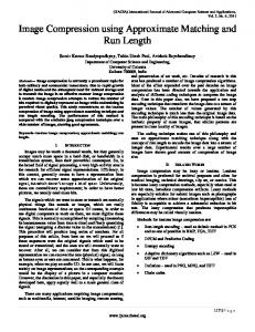
4.1 Fixed Length Keys: Hamming Case The Hamming distance for two strings of length m is de ned as the number of symbols in identical positions that are dierent. For example, Ham(string; strong) is 1. For two strings a and b of size m we have 0  Ham(a; b)  m A string can be also seen as a point in an m-dimensional space with integer coordinates in the set f1; 2; :::; j jg. The Hamming metric can be computed in O(m) time. We assume here that all strings have the same length m and that each key symbol is drawn independently from the alphabet  . Let q = 1 ? 1= be the probability that two symbols dier. The probability that the distance between two elements a and b is k is given by the binomial distribution   pk (m; ) = PrfHam(a; b) = kg = mk qk (1 ? q)m?k with 0  k  m. The maximum value of pk (m; ), the mode, is given by k such that pk  pk?1 and pk > pk+1. Solving these equations we get mq ? q  k  mq ? q + 1. That is, k is very close to the expected value of the distribution which is mq. So, using k = ( ? 1)m= we obtain the following upper bound when  is nite and m is large H (n)  2(1 + O(1= log m)) logm n similarly to random m-ary tries [GBY91]. It is dicult to obtain other closed expressions given the complexity of the analysis. Using the formula for ND (n) we can compute the values for , which gives the complexity of PD (n) = O(n). Figure 2 shows the values for  in a proximity searching for dierent values of m and D with  = 4. We also include experimental values for  (dotted lines) obtained by using a least squares t on the data. Using the probability distribution pk we can compute all the performance measures using the formulas of the previous section. Figure 3 shows analytical and experimental values for proximity searching (PD (n)) in

function of n for dierent values of D when  = 4 and m = 16. Experimental values are given by the dotted lines (as in all the other graphs) and agree reasonable well with the analysis. We have used a logarithmic y-axis to be able to represent several values of D in the same graph (the same occurs in subsequent graphs). Figures 4 and 5 shows the the eect of the key length and the alphabet size for proximity searching. When m increases, the number of comparisons decrease. This happens because the fan-out of the tree increases. On the other hand, when  increases the number of comparisons does the same. This happens because the probability distribution of the possible distances concentrates near the average (approaching m) and the average fan-out decreases. Figure 6 shows the eect of the bucket size b on H (n) and I (n) for m = 16,  = 4, and n = 90000. Figure 7 shows the eect of the bucket size on PD (n) (solid lines) for n = 90000 with m = 16 and  = 4. Clearly, the optimal bucket size is b = 1. Using the formulas for BD (n) and ND (n) we can compute how much we are saving with respect to BK-trees by not having to do one comparison per internal node, which would give BD (n) + ND (n) instead of PD (n). Figure 7 shows also this quantity (dashed lines), and that the improvement over BK-trees is more than 50% for small b. We also have experimental results for nding the closest match, and for that case, the number of comparisons after some point decreases with n. This is due to the fact that for larger n the probability of nding a close match increases, which prunes the tree search more rapidly. The experimental results were obtained by using random keys and running between 10 and 50 experiments, depending on the complexity measure. The largest variation was obtained for the height (as expected). For example, the experimental value for H (90000) with  = 4, m = 16, and b = 2 was on average 9:80 with a standard deviation of 0:42. In other measures the deviation was less than 1%. For almost all the gures given, the experimental results are very close to the approximated analytical values.

4.2 Variable Length Keys: Levenshtein Case The Levenshtein distance is de ned as the minimal number of characters that we need to change, insert, or delete to transform one of the strings into the other string. For example, Lev(string; song) is 3. For two strings a and b we have 0  Lev(a; b)  max(jaj; jbj) The Levenshtein distance can be computed in time O(jaj  jbj) by using dynamic programming. We model the variable length key by generating independently the length of each key. We use a positive Poisson distribution with parameter  for the length. This distribution models the fact that shorter strings are more probable than very long strings. Let Li be the probability of a string a having length i > 0, then i?1 Li = Prfjaj = ig = (i? 1)! e? The distance between two strings a and b is computed by using the length dierence of the two elements and for the common pre x of length m = min(jaj; jbj), because both strings are random, we use the Hamming distance. So, without losing generality we have Lev(a; b) = jjaj ? jbjj + Ham(a1 :::am; b1:::bm): But we know already the probability distribution pk for the Hamming distance. Thus, the probability of Lev(x; y) being k is

0 X @ Pk = Li i1

Xi

j =max(1;i?k)

Lj pk?(i?j )(j; ) +

i+k X j =i+1

1 Lj pk?(j ?i)(i; )A

P

Because the distance can be unbounded, we de ne Pk0 = Pk for k < s = 2, and Ps0 = 1 ? ks?=01 Pk . With this probability distribution P 0 we can compute all the performance measures de ned in the previous section

as in the Hamming case. For example, Figure 8 shows the complexity of proximity searching for some values of D and  (average string length) for  = 30 (a simple model for lower case text). Figure 9 shows the eect of n on proximity searching for  = 5 and  = 30. The results are similar to the Hamming case with  replacing m. The main dierence in this case is that the probability distribution is more centered than for the Hamming case. We are currently working on experimental results for this distance function.

5 Conclusions and Future Work In this preliminary paper we introduced FQ trees and showed their potential as a data structure that supports fast approximate queries. The novelty of FQ trees is having one xed key per level to lter the input. This idea is obviously not generally applicable because it leads to traversal of many nodes. However, as we showed, the number of key comparisons is decreased by using our data structure. More work is necessary to see how FQ-trees compare to other data structures for speci c applications in which comparing two elements is the major cost of the search. Also, an exact analysis would be desirable. We mention brie y here one important variant of FQ-trees that takes the tradeo of reducing the number of key comparisons vs. increasing the number of traversed nodes even further. Instead of building the tree recursively and stopping when a node contains no more than b elements, we can insist that every leaf has no less than a certain depth. In other words, we may want to replace leaves with paths. When we arrive at a leaf that contains even one element, there is no guarantee than this element ts the search criteria. We still need to compare the element directly to the query adding one more key comparison. But if we add more levels to a leaf, we increase the probability that the triangle inequality will lter out the element corresponding to that leaf. So, we will traverse more nodes, but at the end we will be left with a smaller set to compare directly to the query. And since we insist on one key per level, the total number of key comparisons will be signi cantly reduced. A preliminary analysis shows that in expectation it is possible to achieve logarithmic number of key comparisons for a xed small D. (The performance degrades signi cantly when D is increased.) Preliminary experimental data supports this analysis. It is too early, however, to predict whether this variant will be practical. There are several other ways to improve and extend the basic idea of FQ-trees:  The key selection, which we did at random, can be adapted to the data. For example, if the data is known to be divided into clusters, then one key per cluster is a good choice.  Elements can be partitioned into smaller objects to allow local similarity. For example, for sequence comparisons we can divide each sequence into smaller sequences and treat each smaller part as an element. We will do the same for the query and search each part separately.  Further study is needed to optimize the use of secondary memory and to improve the bucket utilization. It may be possible to have partial split procedures that improve storage utilization similarly to multiway trees [BYC92].

Acknowledgements We would like to thank the helpful comments of the referees.

References [AGMML90] Altschul S.F., W. Gish, W. Miller, E. W. Myers, and D. J. Lipman, \Basic local alignment search tool," J. Molecular Biology 15 (1990), 403{410.

[BYC92] Baeza-Yates, R.A. and Cunto, W., \Unbalanced Multiway Trees Improved by Partial Expansions", Acta Informatica, 29 (5), 1992, 443{460. [BYG90] Baeza-Yates, R.A. and Gonnet, G.H., \All-against-all Sequence Matching", Dept. of Computer Science, Universidad de Chile, 1990. [BGKN90] Bahl L. R., P. S. Gopalakrishnan, D. S. Kanevsky, and D.S. Nahamoo, \A fast admissible method for identifying a short list of candidate words," IBM tech report RC 15874 (June 1990). [BR+93] Bugnion, E. and Roos, T. and Shi, F. and Widmayer, P. and Widmer, F. \A Spatial Index for Approximate Multiple String Matching", 1st South American Workshop on String Processing, Belo Horizonte, Sept 1993, 43{54. [BK73] Burkhard, W.A. and Keller, R.M. \Some Approaches to Best-Match File Searching", Communications of the ACM 16 (4), April 1973, 230-236. [CL90] Chang W.L., and E.L. Lawler, \Approximate matching in sublinear expected time," Proc. of the 31st IEEE Symp. on Foundations of Computer Science (1990) 116{124. [FBF77] Friedman, J.H. and Bentley, J.L. and Finkel, R.A. \An Algorithm to nd best matches in logarithmic expected time", ACM Trans. on Math. Software 3(3), 1977. [GBY91] Gonnet, G.H. and Baeza-Yates, R. Handbook of Algorithms and Data Structures, Addison-Wesley, second edition, 1991. [GCB92] Gonnet, G.H., M.A. Cohen, and S.A. Benner, \Exhaustive matching of the entire protein sequence database," Science 256, 1443. [LP85] Lipman D. J., and W.R. Pearson, \Rapid and sensitive protein similarity searches," Science 227 (1985), 1435-1441. [Mah92] Mahmoud, H. Evolution of Random Search Trees, John Wiley, New York, 1992, [Mur83] Murtagh, F. \A Survey of Recent Advances in Hierarchical Clustering Algorithms", IEEE Computer 26 (4), 1983, 354{359. [My92] Myers, E. \Algorithmic Advances for Searching Biosequence Databases," Proceedings of the International Symposium on Computational Methods in Genome Research (Heidelberg, 1992), to appear. [My94] Myers, E. \A Sublinear Algorithm for Approximate Keyword Matching," Algorithmica, in press. [NK82] Nevalainen, O. and Katajainen, J. \Experiments with a Closest Point Algorithm in Hamming Space", Angewandte Informatik 5, 1982, 277-281. [SDDR89] Santana, O. and Diaz, M. and Duque, J.D. and Rodriguez, J.C. \Increasing radius search schemes for the most similar strings on the Burkhard-Keller tree", International Workshop on Computer Aided Systems Theory, EUROCAST'89, 1989. [Sha77] Shapiro, M. \The Choice of Reference Points in Best-Match File Searching", Communications of the ACM 20 (5), May 1977, 339{343. [SW90] Shasha, D. and Wang, T-L. \New Techniques for Best-Match Retrieval", ACM Transactions on Information Systems 8, 1990, 140{158. [Uk92] Ukkonen, E., \Approximate string matching with q-grams and maximal matches," Theoretical Computer Science (1992), 191{212. [Uk93] Ukkonen, E., \Approximate string-matching over sux trees," 4th Annual Combinatorial Pattern Matching Symp., Padova, Italy (June 1993), 228{242.

This article was processed using the LATEX macro package with LLNCS style

1.00 + + 0.95 + 0.90 0.85 +

 0.80

+ + + +

0.75

+ +

+ +

+ +

+

+ +

+

+

+

+

+

+

+

0.70 0.65 0.60

+

0.55 0.50 0.45

10

+

12

+ 14

+

+

+

+ + + +

+

+ +

+ +

+

+

+

+

+

+

+

+D = 3

+

+

+ 28

+

D=2

D=1

18 20 22 24 26 30 Key length (m) Fig. 2. Complexity of proximity searching depending on D and m (Hamming). Experimental results are shown with dotted lines and + symbols. 65000 40000

16

+

+D = 5 D=4 +

+

D=4

20000 10000

+ +

PD (5000 n)

+ + +

2000

+

1000

+ +

D=3 + D=2

+ +

+ +

100

+ 0

+ 20000

+ D=1

+

+

+

+

+

+

+

+

+

+

+

+

+

+

+

+

+

+

+

+

+

+

+

500 200

+

40000 60000 80000 100000 Number of elements (n) Fig. 3. Eect of n on proximity searching depending on D for m = 16,  = 4 and b = 1 (Hamming). Experimental results are shown with dotted lines and + symbols.

60000 + 40000

+

D=3

20000 +

+

10000

PD

+ +

D=2

+

+

+

+

5000 2000 1000

+

+

+

D=1

500 200

10

12

+

+

+

+

+

+

+

+

+

+

+

+

18 20 22 24 26 Key length (m) Fig. 4. Eect of key length on proximity searching depending on D for  = 4, b = 3 and 90000 elements (Hamming). Experimental results are shown with dotted lines. 90000 60000 40000 +

20000

+

+

PD10000

14

+

+

+

16

D=3 + +

+ + D=2

+

+

+

+

+

+

+

+

5000

D=1 2000 1000 500

+

+

+ 2

4

6

+ 8

+

10

+

12

+

+

+

+

+ +

+

+ +

+

+ +

+

+ +

+ +

+

+

14 16 18 20 22 24 26 28 30 Alphabet size () Fig. 5. Eect of alphabet size on proximity searching depending on D for m = 20, b = 3 and 90000 elements (Hamming). Experimental results are shown with dotted lines.

10

+ +

9

+

8 7

+ +H (n)

+ +

6 5

+

1

+

2

+

+

+

+I (n)

4 5 6 7 Bucket size (b) Fig. 6. Height and internal path depending on b for 90000 elements (Hamming). Experimental results are shown with dotted lines and + symbols.

15000 10000 5000

PD

+

3

+

D=2

+

+

+

+

+

+

+

+

+

+

2000

D=1

1000 +

500 1

2

3

4 5 6 7 Bucket size (b) Fig. 7. Eect of the bucket size on proximity searching for 90000 elements (Hamming). Experimental results are shown with dotted lines and BK-trees are shown with dashed lines.

0.95 0.90 0.85 0.80 0.75  0.70 0.65 0.60 0.55 0.50 0.45 0.40

D=3 D=2

D=1 4

5

6

7 8 9 10 11 12 Key length () Fig. 8. Complexity of proximity searching depending on D and  (Levenshtein).

40000

D=4

20000 10000 5000

D=3

PD 2000

D=2

1000 500

D=1

200 0

20000

40000 60000 80000 100000 Number of elements (n) Fig. 9. Eect of n on proximity searching depending on D for  = 5,  = 32 and b = 1 (Levenshtein).