Request For Comments 1889, 1996. [15] Ellen W. Zegura, Ken Calvert and S. Bhattacharjee, âHow to Model an Internetwork,â in INFOCOM '96, 1996. [16] Y. Guo ...
Proxy-based Asynchronous Multicast for Efficient On-demand Media Distribution Yi Cui, Klara Nahrstedt Department of Computer Science University of Illinois at Urbana Champaign {yicui, klara}@cs.uiuc.edu Abstract To achieve scalable and efficient on-demand media distribution, existing solutions mainly make use of multicast as underlying data delivery support. However, due to the intrinsic conflict between the synchronous multicast transmission and the asynchronous nature of on-demand media delivery, these solutions either suffer from large playback delay or require clients to be capable of receiving multiple streams simultaneously and buffering large amount of data. Moreover, the limited and slow deployment of IP multicast hinders their application on the Internet. To address these problems, we propose asynchronous multicast, which is able to directly support on-demand data delivery. Asynchronous multicast is an application level solution. When it is deployed on proxy network, stable and scalable media distribution can be achieved. In this paper, we focus on the problem of efficient media distribution. We first propose a temporal dependency model to formalize the temporal relations among asynchronous media request. Based on this model, we propose the concept of Media Distribution Graph (MDG), which represents the dependencies among all asynchronous requests in the proxy network. Then we formulate the problem of efficient media distribution as finding Media Distribution Tree (MDT), which is the minimal spanning tree on MDG. Finally, we present our algorithm for MDT construction/maintenance. Through solid theoretical analysis and extensive experimental study, we claim that our solution can meet the goals of scalability, efficiency and low access latency at the same time.
1 Introduction On-demand media distribution has gained intensive consideration recently due to its promising usage in a rich set of Internetbased services such as media distribution, distance education, video on demand, etc. The primary challenge here is to enable efficient, scalable and on-demand media delivery. By efficient, we mean that the system should make minimum use of media server and network resources. By scalable, we mean that the media distribution system should accommodate a large number of clients dispersed in the wide area. By on-demand, we mean that the client is free to access any portion of the media stream (e.g., fast forwarding and rewind in VoD) and the access latency must be bounded by a small delay time. An ideal media distribution system should meet all the three requirements. To achieve the goal of efficiency, a general approach is multicast. The nature of multicast is synchronous, i.e., data is sent to all receivers simultaneously. However, on-demand media distribution requires data to be delivered in an asynchronous manner, i.e., users want to receive data at different times. To apply multicast in the context of on-demand media distribution, different solutions have been proposed[1][2][3][4][5][6]. In batching[1], asynchronous requests are aggregated into one multicast session to save server and network resources. However, the users have to suffer long playback delay since their requests are enforced to be synchronized. Patching[2][3] tries to address this problem by allowing the client to “catch up” an on-going multicast session and patch the missing starting portion through server unicast. In merging[4], a client can repeatedly merge into larger and larger multicast sessions using the same way as patching. However, in order to ensure smooth playback, these two approaches need the client to be capable of receiving multiple streams simultaneously and buffering large amount of data. In periodic broadcasting[5][6], the server separates a media stream into segments and periodically broadcasts them through different multicast channels, from which a client chooses to join. Although more efficient in saving server bandwidth, it shares the same limitations as previous approaches. Furthermore, all these solutions implicitly assume that users always request a stream from its beginning. How the existing techniques will perform, if the user is allowed to access a random portion of the stream, is still an open question.
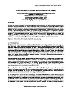
We argue that all these limitations originate from the intrinsic conflict between the synchronous multicast transmission and the asynchronous requirement from on-demand media delivery. Besides the above limitations, these solutions face another problem when deployed in the real world: they all assume the multicast support from underlying network. However, the deployment of IP multicast in the Internet has been slow and severely limited. Recently, application-layer multicast[7][8][9][10] has been proposed to compensate the absence of IP multicast. The main idea is to build an overlay network among end hosts. To enable multicast functionalities, end hosts cooperate with each other to relay data. Current research in this area has not considered applying application-layer multicast in the context of on-demand media distribution yet. Even if this approach is feasible, the original limitations of media delivery techniques that result from the intrinsic conflict between multicast and on-demand delivery still remain unresolved. Based on these observations, we have the following reflections: (1) Multicast does not well fit the application of ondemand data delivery; (2) Limiting on-demand media distribution within the context of IP multicast is not necessary, since it is not widely deployed anyway; (3) If application-layer support is considered, designing mechanisms other than multicast may have the potential to avoid the conflict between synchronous data transmission and the requirement of on-demand media delivery, thus better suit the need of on-demand media delivery and lead to more efficient system designs. From above thinking, we propose a novel mechanism – Asynchronous Multicast, which is able to support on-demand data delivery directly. A conceptual comparison of multicast and asynchronous multicast is shown in Figure 1. Asynchronous multicast is implemented on application-layer overlay network. It relies on peer end host to relay data for each other. The key to asynchronous data transmission is cooperative buffering. By enabling data buffering on the relaying nodes, requests at different times can be satisfied by the same stream, achieving efficient asynchronous media delivery. While impossible in IP multicast since routers can buffer very limited amount of data, it can be realized on the application layer, where relaying nodes are end hosts or proxies with strong buffering capabilities. A comparison of two multicast schemes is shown in Figure 1. t2 t1 t0
On-demand media delivery techniques ( batching, patching, )
On-demand delivery
t0
Synchronized transmission
On-demand delivery
IP multicast
Asynchronous multicast
(a) Conceptual Comparison
t4 t3 t0 t0
t0 t0
t4
t2
t1 t3
(b) Multicast Tree Comparison
Figure 1: Comparison of IP Multicast and Asynchronous Multicast Asynchronous multicast is superior to the existing media distribution techniques in the following aspects: (1) With the aid of buffering, clients with asynchronous requests can reuse the same media stream. (2) The client request is immediately satisfied by the intermediate node, which keeps the requested data in its buffer. (3) The client is not required to receive multiple streams simultaneously and buffer them to ensure smooth playback. Instead, it only receives one stream as requested. (4) The client can request a stream from any starting point, instead of always from beginning. (5) It is an application-layer solution which does not requires any changes to the existing underlying network. In this paper, we present a proxy-based overlay network to support asynchronous multicast. In particular, we design and evaluate an on-demand media distribution system on top of this proxy overlay network. Our solution is summarized as follows: (1) We propose a temporal dependency model to model temporal relations among asynchronous requests. We reveal that for two asynchronous requests R1 and R2 for the same media stream, if R1 receives data earlier than R2 , then R1 has the potential to benefit R2 , in that R2 could reuse the same stream from R1 . (2) We deploy our model in a proxy-based framework. In this framework, proxies serve as the intermediate buffering nodes in media delivery. We argue that stable and scalable media distribution can be achieved through proxy-based network. (3) Under the temporal dependency model and its deployment framework, we formulate the problem of efficient on-demand media distribution into a graph problem. In particular, we propose two concepts: (a) Media Distribution Graph (MDG), which represents the dependencies among all asynchronous requests in the proxy network; (b) Media Distribution Tree (MDT), which is a spanning tree on MDG. The optimal solution for efficient data distribution is to construct and maintain the optimal MDT for a given MDG, which is a Minimal Spanning Tree. (4) We further refine this problem into two subproblems: (a) how to construct and maintain the optimal MDT; (b) how to acquire necessary knowledge, which will facilitate the construction/maintenance of MDT. To
address the first problem, we present a distributed algorithm for MDT construction/maintenance. The algorithm is proved to be correct and optimal. For the second problem, we design an efficient content discovery scheme to facilitate the acquisition of necessary knowledge information. Through solid theoretical analysis and extensive experimental study, we claim that our solution can meet the scalable, efficient and on-demand requirements at the same time. To summarize, the main novelties and contributions of this paper include: (1) The concept of asynchronous multicast, a novel application-layer solution for efficient, large scale, on-demand media delivery; (2) The temporal dependancy model, which formalizes the temporal relationship among asynchronous requests; (3) A fully distributed and incremental MDT construction and maintenance algorithm; (4) An efficient and distributed content discovery scheme through hashing functions. The rest of this paper is organized as follows. Section 2 introduces the temporal dependency model and presents its deployment framework. Section 3 formulates the problem. Section 4 presents the algorithm for MDT construction/maintenance and content discovery. Section 5 presents the performance evaluation. Section 6 discusses the related work. Section 7 concludes the paper.
2 Model 2.1
Temporal Dependency Model
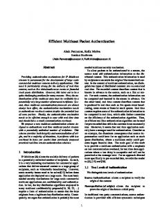
Consider two asynchronous requests Ri and Rj for the same video file1 . The time length of the video file is Vh . Ri happens at time ti and requests the video starting at the offset Vi . Rj happens at time tj and requests the video starting at the offset Vj (0 ≤ Vi , Vj < Vh ). We introduce the following definition to model their temporal dependency. Definition 1: Given two requests Ri and Rj . If ti − Vi < tj − Vj , Ri is the predecessor of Rj , Rj is the successor of Ri , denoted as Ri ≺ Rj . As an example, in Figure 2 (a), R1 ≺ R2 . From the definition we can see, if R1 is the predecessor of R2 . R1 has the potential to benefit R2 in that, R2 could reuse the stream from R1 instead of getting another one directly from the video server. To achieve this, we need to let the playback stream R1 be buffered. Clearly, the larger the buffer size, the more requests R1 can possibly benefit. However, in practice, the buffer size needs to be bounded. Thus, only requests that fall into the buffer could be really benefited. To model such “constrained temporal dependency”, we introduce the following definition: Vh
Vh
V1+t2-t1
V2 V1
R2
R1
Stream played by R1
R1
R B(
R2
R3
)
1
V2 V3 V1
t1
t2
t3
time
(a) Basic Temporal Dependency
t1
t2
t3
time
(b) Buffer-based Temporal Dependency
Figure 2: Temporal Dependency Model Definition 2: Given two requests Ri and Rj so that Ri ≺ Rj . Let B(Ri ) be the buffer allocated for Ri , and Size(B(Ri )) be the time length of B(Ri ). If ti − Vi + Size(B(Ri )) ≥ tj − Vj , Ri is the constrained predecessor of Rj , Rj is the constrained successor of Ri , denoted as Ri
B(Ri )
≺ Rj .
B(R1 )
As shown in Figure 2 (b), only R1 ≺ R2 . So R2 can get the stream from the host where the buffer for R1 is located. By doing so, we can reduce the server load and save the network transmission cost (if the cost of streaming data from R 1 to R2 is less than from the server to R2 ). V3 falls out of the buffer range, thus it can not benefit from R1 . Note that our model uses the circular buffer to cache the stream. It means that any data cached in the buffer B(R 1 ) is kept for a time length of Size(B(R1 )), after which it is replaced by the new data. In other words, a window of size Size(B(R 1 )) is kept along the video playback for R1 , and all requests falls within this window can be served. Furthermore, the buffer is discarded when 1 We use video distribution as an example to illustrate our framework, which can be applied to any type of streaming-based multimedia content. In the rest of this paper, we use term video and multimedia content interchangeably.
the streaming is over. This distinguishes our model from other prefix-caching[11] or segment-caching[12] schemes, where the buffer content is permanent and fixed. In this paper, we only consider buffer with fixed size 2 . Thus, we can simply denote b = Size(B(Ri )) .
2.2
Model Deployment: Cooperative Proxy Overlay Network
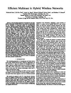
Our temporal dependency model could be deployed in two types of frameworks: client-based or proxy-based. In clientbased framework, each client buffers the stream locally and serves other clients using its buffered data. In this way, a media distribution overlay network is formed among cooperative clients. However, in practice, the client-based framework is not suitable for large-scale media distribution for the following reasons: First, maintaining an overlay network scalable enough for a large number of client nodes is a difficult task; Second, the clients’ heterogeneity and highly unpredictable nature (machine crash, constant leaving/joining the network) will complicate group management and make streaming between clients highly unstable. In the proxy-based framework, proxies buffer data on behalf of clients. Currently in the Internet, proxies are often deployed at the head-end of the local network, serving clients within the same domain. Obviously, proxies have stronger network connectivity and buffering capabilities than clients. Their stability and availability are also much better than clients. Thus, we consider this type of framework in the paper. In proxy-based framework, clients from different domains are organized into non-overlapping groups. Each group of clients is uniquely assigned to a proxy. Once a client issues a stream request, it is first intercepted by its proxy. If the requested data is available on the proxy, it is streamed to the client directly. Otherwise, the proxy requests it from the server or other proxies, and then relays the incoming data to the client. At the same time, proxy buffers the playback stream on behalf of the client. The client is merely a consumer and does not buffer any data. Thus, an overlay network is formed among proxies, which cooperate with each other in media delivery. We refer this network as cooperative proxy overlay network in this paper. We use a sample scenario to illustrate the on-demand media streaming in our cooperative proxy overlay network. Let us consider a simple server-proxy-client hierarchy shown in Figure 3 (a). S is the server, P 1 , P2 and P3 are proxies serving client groups {C1 , C2 }, {C3 , C5 } and {C4 } respectively. The temporal dependencies among different requests are shown in Figure 3 (b). R1 from client C1 is intercepted by P1 . P1 forwards R1 to S and then relays the stream from S to C1 . P1 B(R1 )
also caches the stream in its local buffer B(R1 ) on behalf of C1 . Since R1 ≺ R2 , P1 can directly send data to C2 from its local buffer B(R1 ), when C2 issues R2 to it. When R3 from C3 is intercepted by P2 , P2 will issue a request among B(R1 )
proxies and servers for R3 . Since R1 ≺ R3 , P2 can retrieve the stream from B(R1 ) at P1 . Upon forwarding the stream to C3 , P2 also allocates a new buffer B(R3 ). Similarly, R4 from C4 is intercepted by P3 , then satisfied by B(R3 ) since B(R3 )
R3 ≺ R4 . When R5 is intercepted by P2 , P2 will issue a new request, since its existing buffer B(R3 ) can not satisfy R5 . This request is directly served by S since R5 cannot benefit from any existing buffers among the proxy network. From the picture, we can see there are two types of requests: intra-proxy request (or client request) and inter-proxy request( or proxy request). Clients issue intra-proxy requests, if they can be directly served by a local buffer of their proxies, the request is masked, such as R2 . Otherwise, an inter-proxy request is triggered, such as R1 , R3 , R4 and R5 . In this paper, we mainly study the inter-proxy requests problem, since client requests are resolved locally. To enforce efficient media distribution, we consider the following questions: (1) Upon a proxy request, how does a proxy know which proxies have the stream it demands? (2) how does a proxy buffer choose the “best buffer” to retrieve the stream, if there exist multiple proxy buffers which can satisfy its request? These problems are formulated in the next section. S
Vh
R1
R2
R3
R4
S
R5
R1 R5 V5
P1
P2
R B(
P3
)
R B(
1
P1
)
C2
C3
C5
C4
(a) Server-Proxy-Client Hierarchy
B(R4) R3
R1 R2
B(R3) R3
R4 R5
R4
time t1
t2
t3
t4
t5
(b) Request Temporal Dependencies
Figure 3: Sample Scenario 2 The
P3
B(R5)
B(R1)
V4 V3 V2 V1
C1
P2
3
buffer size is a design parameter. We evaluate its impact in our simulation study.
C1
C2
C3
C5
(c) Data and Request Flow
C4
3 Problem Formulation 3.1
Temporal Dependency between Proxy Buffers
As revealed in Section 2, each proxy request triggers the allocation of a proxy buffer. To facilitate the problem formulation, we use the temporal dependency between two buffers to represent the dependency between their corresponding requests. B(Ri )
Definition 3: Given two proxy requests Ri and Rj , and their buffers B(Ri ) and B(Rj ). If Ri ≺ Rj , then B(Ri ) is the predecessor of B(Rj ), B(Rj ) is the successor of B(Ri ), denoted as B(Ri ) ≺ B(Rj ), or simply Bi ≺ Bj .
3.2
Media Distribution Graph
Let B be the set which includes all proxy buffers. We define the Media Distribution Graph (MDG) for B as a directed weighted graph M DGB = (B, E), such that E = {(Bi , Bj ) | Bi ≺ Bj , Bi , Bj ∈ B}. Each edge (Bi , Bj ) has the weight w(Bi , Bj ), which is the transmission cost between two proxies carrying Bi and Bj respectively. A sample MDG is illustrated in Figure 4. As shown in Figure 4 (a), in MDG, each node represents a buffer 3 . An edge directed from node B1 to B3 means that B1 is the predecessor of B3 , i.e., B3 could reuse the media stream from B1 . w(B1 , B3 ) is the transmission cost between proxies P1 and P2 , which hold B1 and B3 respectively. A special node is Bserver representing the server. Since the server can serve any proxy request, it is the predecessor of all other buffers. Thus, B server has directed edges to all other nodes in the graph. MDG is changing dynamically: (1) a new buffer is allocated when a new request arrives, thus a new node is inserted into the graph; (2) a buffer is discarded when its streaming session is over, thus the corresponding node is removed from the graph. In summary, MDG represents the dependencies among all asynchronous requests and their resulting buffers in the proxy network, which forms a virtual overlay on top of proxy overlay network. The weight of edges in MDG reflects the communication cost from the physical proxy networks. B5
B3 B4
Bserver B1
P2
S P1
P3
Media Distribution Graph
Bserver
B1
Proxy Overlay Network
B5
MDG Edge Buffer Proxy
Physical Network
Router
(a) Media Distribution Graph
B3
B4
MDG Edge MDT Edge
(b) Media Distribution Tree
Figure 4: Illustration of Media Distribution Graph
3.3
Media Distribution Tree
Given the definition of MDG, the efficient media distribution problem can formulated as constructing and maintaining a spanning tree on the MDG, as shown in Figure 4 (b). We define such a spanning tree as Media Distribution Tree. Formally, for a buffer set B and its MDG M DGB = (B, E), the corresponding MDT is denoted as M DTB = (B, E T )(E T ∈ E). For two nodes Bi , Bj ∈ B, if (Bi , Bj ) ∈ E T , then Bi is the parent of Bj , Bj is the child of Bi . Given a MDG, the optimal solution for MDT, i.e., to minimize the overall transmission cost of media distribution, is to find the Minimal Spanning Tree (MST) on MDG. Note that existing algorithms for MST can not be directly applied to our problem for the following reasons. First, our solution does not assume the existence of centralized manager, which has the global knowledge and controls the tree construction. Instead, we needs the tree to be constructed in a fully distributed manner. Second, since MDG is constantly updated, the corresponding MDT maintenance must be incremental. Frequent tree reorganization will incur unacceptable overhead. As will be presented in Section 4, our MDT algorithm satisfies the above requirements. 3 We
use the term buffer and node interchangeably in the remainder of this paper, depending on the context.
4 Efficient Media Distribution In this section, we present our solution on MDT construction/maintenance. We present the algorithm in Section 4.1, and its distributed implementation in Section 4.2. Given a MDG, the algorithm is able to constantly maintain its MDT as the graph is dynamically updated. To achieve so, the algorithm requires that each node in the MDG have the up-to-date knowledge about its neighbors. Section 4.4 introduces a content discovery scheme, which facilitates the acquisition of such knowledge.
4.1
Algorithm
Our algorithm makes the following assumptions. (1) For a given buffer set B and its MDG M DG B , each node in M DGB has the knowledge of its in-bound and out-bound neighbors. (2) We assume that for any edge (B i , Bj ) ∈ E, w(Bi , Bj ) is known to Bi and Bj . We further assume that w(Bi , Bj ) changes over long period, compared to the time length of data streaming between Bi and Bj . It means that the transmission cost between the proxies carrying Bi and Bj is stable. Our assumption is validated by the fact that a proxy relies on the underlying network routing mechanism to send the data to another proxy. Therefore, the network route between two proxies is stable or changed slowly. Our algorithm has the following properties: (1) It is fully distributed. The MDT construction/maintenance is made by the local node. No centralized manager is required. (2) The MDT construction/maintenance is incremental. In case of node join/leave, only a portion of the tree is affected. No global tree reorganization is needed. (3) The algorithm guarantees to return the optimal result, as will be proved in Section 4.3. The algorithm is executed each time when a new node joins the graph, or when an old node leaves. To deal with these two cases, our algorithm has two operations: MDT-Insert and MDT-Delete. Actually, MDT can be constructed incrementally by repeating MDT-Insert. We first consider the case of node insertion. Let M DGinsert = (B ∪ Binsert , Einsert ) be the resulting graph after T Binsert and its inducing edges are added to M DGB , MDT-Insert is able to return M DTinsert = (B ∪ Binsert , Einsert ) as the new MDT for M DGinsert . T MDT-Insert(Binsert , Einsert , E T , Einsert ) /∗ From all its predecessors, Binsert finds its parent Bmin , whose transmission cost to Binsert is minimal ∗/ 1 P (Binsert ) ← {Bpred | (Bpred , Binsert ) ∈ Einsert } 2 wmin ← min{w(Bpred , Binsert ) | Bpred ∈ P (Binsert )} T 3 Einsert ← E T ∪ {(Bmin , Binsert ) | w(Bmin , Binsert ) = wmin }
/∗ For all its successors Bsucc , Binsert compares if the transmission from itself to Bsucc is less than from Bsucc ’s current parent Bparent . If so, Bsucc is asked to switch parent to Binsert . ∗/ 4 for each Bsucc ∈ {Bsucc | (Binsert , Bsucc ) ∈ Einsert } 5 if w(Binsert , Bsucc ) < w(Bparent , Bsucc ) ∈ E T T T 6 do Einsert ← (Einsert − (Bparent , Bsucc )) ∪ {(Binsert , Bsucc )} Now we discuss the case of node leaves. Suppose the existence of M DGB = (B, E) and its MDT M DTB = (B, E T ). A node Bdelete leaves from M DTB . Let M DGdelete = (B − Bdelete , Edelete ) be the resulting graph after Bdelete and its T inducing edges are removed from M DGB , MDT-Delete is able to return M DTdelete = (B − Bdelete , Edelete ) as the new MDT for M DGdelete . T MDT-Delete(Bdelete , Edelete , E T , Edelete ) /∗ Bdelete deletes the tree edge from its parent Bparent ∗/ T 1 Edelete ← E T − {(Bparent , Bdelete ) | (Bparent , Bdelete ) ∈ E T } 2 for each Bchild ∈ {Bchild | (Bdelete , Bchild ) ∈ E T } do /∗ Bdelete deletes the tree edge to each of its children Bchild ∗/ T T 3 Edelete ← Edelete − (Bdelete , Bchild ) /∗ From all its predecessors, Bchild finds the new parent Bmin , whose transmission cost to Bchild is minimal ∗/ 4 P (Bchild ) ← {Bpred | (Bpred , Bchild ) ∈ Edelete } 5 wmin ← min{w(Bpred , Bchild ) | Bpred ∈ P (Bchild )} T T 6 Edelete ← Edelete ∪ {(Bmin , Bchild ) | w(Bmin , Bchild ) = wmin }
We use an example to illustrate the MDT algorithm. Initially, we have a buffer set B = {B server , B1 , B2 , B3 , B4 } and the corresponding MDT. B5 first arrives, which runs MDT-Insert. Then B3 leaves the MDT, which runs MDT-Delete. Finally, B6 is inserted, which runs MDT-Insert. The whole process is illustrated in Figure 5. Bserver
Bserver
5 3
3
6
6
2
1
5
(a) Before insertion of B5
B1
1
B1
3 B6
7
5 B5
(b) After insertion of B5
3 B6
7 6
2
2
B2
B4
5
B5
B1
6
2
6 4
2
2
6 B4
B2
5
6 4
3 B4
B2
3
6
2
1 3
B4
B5
B3
Bserver
5 4
6
2
3 B2
3
B1
Bserver
5
4 4
B3
B1
Bserver
5
4 4
B3
B1
Bserver
5
4 4
(c) Before deletion of B3
B2
5
B2
B4
5
B5
(d) After deletion of B3
6 B4
B5
(e) Before insertion of B6
5 B5
(f) After insertion of B6
Figure 5: A example illustrating the MDT Algorithms
4.2
Distributed Implementation
In practice, our algorithm is implemented in a fully-distributed fashion, i.e., the MDT construction/maintenance decision is made locally by each buffer. Information Required Each buffer Bi ∈ B carries the following information: its own parent P arent(Bi ) and its child list Childlist(Bi ). Bi also needs to know the transmission cost between itself and any other buffer. This can be achieved by asking the proxy carrying Bi to keep track of its transmission cost to all other proxies. Note that the acquisition of such information will not trigger additional overhead since two proxies rely on the underlying network routing mechanism to communicate. Thus, the transmission cost between two proxies can be their routing information, such as delay, or simply hop count. Since the network route between two proxies is stable or changed slowly, the above information does not need to be frequently updated. Finally, Bi needs to acquire the knowledge of its neighbors in the MDG, namely its predecessors and successors. To achieve so, Content Discovery Service is required. The service collects information about each buffer in the MDG and answers queries. Here we define two types of functions: query functions and update functions. Query functions include the following: 1. GetP redecessors(Bi ): called by Bi , the function returns all predecessors of Bi . 2. GetSuccessors(Bi ): called by Bi , the function returns all successors of Bi . The update functions include the following: 1. Register(Bi ): Bi calls this function to register itself to the discovery service when it is newly allocated. B i provides information such as its residing proxy, its parent P arent(Bi ) and the transmission cost from P arent(Bi ) to Bi . 2. Deregister(Bi ): Bi calls this function to remove itself from the discovery service when it is discarded. The implementation of the content discovery service and the above functions will be presented in Section 4.4. Message Exchange During the process of MDT-Delete, first, Bdelete sends out child-leave message to its parent P arent(Bdelete ). On receiving the message, P arent(Bdelete ) stops streaming to Bdelete and removes it from its child list. Second, Bdelete sends out parent-leave message to each buffer in Childlist(Bdelete ) and stops streaming to it. Then Bdelete calls Deregister(Bdelete ) and leaves. For each child Bchild , on receiving the message, it first calls the function GetP redecessors(Bchild ). After receiving a list of buffers which are qualified as its parent, Bchild compares the transmission cost from each of them to itself (by comparing the transmission cost from these buffers’ residing proxies to the proxy where B child is allocated) and finds out the one with minimal cost: Bmin . Finally, Bchild sends out a child-join message to Bmin . Upon receiving the message, Bmin adds Bchild into its child list and start streaming to Bchild . Upon receiving the stream, Bchild sets Bmin as its new parent and calls Register(Bchild ). The whole process is finished after every Bchild orphaned by Bdelete has found its new parent.
During the process of MDT-Insert, first, Binsert finds its parent using the same way as Bchild does in MDT-Delete and calls Register(Binsert ). Then, Binsert calls the function GetSuccessors(Binsert ) to find if any existing buffers are the successors of Binsert . This case may happen as shown in Figure 6. Although Binsert is allocated later than Bsucc , it is still the predecessor of Bsucc since Vinser is ahead of Vsucc . In this case, Binsert first compares if the transmission cost from itself to Bsucc is smaller than the transmission cost from P arent(Bsucc ) to Bsucc (obtained from the query function GetSuccessors(Binsert )). If so, Binsert sends a parent-join message to notify Bsucc to switch to a better parent. Note that as shown in Figure 6, this message is issued at time tinsert , when Binsert is initiated. However, Binsert cannot benefit Bsucc immediately until the time tswitch . Therefore, Bsucc waits until the time tswitch to send a child-join message to Binsert . Binsert then adds Bsucc to its child list and starts streaming to Bsucc . When receiving the stream, Bsucc updates Binsert as its new parent, then calls Register(Bsucc ) to update its information to the discovery service. Vh
rt se
B in
cc
B su
Vinsert
Vsucc tsucc tinsert
tswitch
time
Figure 6: Temporal Dependency between Binsert and Bsucc
4.3
Analysis
We prove the correctness and optimality of MDT-Insert and MDT-Delete as follows. Correctness Lemma 1: MDG is Directed Acyclic Graph (DAG). Proof: By Definition 1-3, Bi ≺ Bj if and only if ti − Vi < tj − Vj . Therefore, a loop Bi → . . . → Bk → Bi in M DGB would mean that ti − Vi < . . . < tk − Vk < ti − Vi , which forms contradiction. Thus M DGB is a DAG. ¥ Theorem 1: MDT-Insert and MDT-Delete are guaranteed to return loop-free spanning trees. Proof: At line 3, MDT-Insert adds one edge (Bmin , Binsert ) to the original tree. On the contrary, MDT-Delete deletes one edge at line 1. For the rest operations, both algorithms only replace old edges with new edges sharing the same destination. Therefore, the inbound degree of these nodes remains unchanged as in the old spanning tree. To this end, we conclude that both algorithms ensure the newly formed tree to have |B| − 1 edges. Moreover, every node except B server in the tree is ensured to have and only have one inbound edge. Thus the tree must cover every node of M DG B . Now we prove that the newly formed tree is loop-free. We only need to prove that M DG B from where the tree is derived is loop-free, which is proved by Lemma 1. ¥ Optimality Before proving the optimality of our algorithms, we first consider the problem of constructing MDT on a static MDG. Suppose the existence of M DGB = (B, E), the algorithm MDT-Construct is able to return the MDT for M DGB , which is M DTB = (B, E T ). Lemma 2: MDT-Construct creates the MST. Proof: We use induction to prove that the algorithm always keeps a MST among those nodes dequeued from Q so far. We organize these nodes into a temporary graph G0 = (B0 , E 0 ), where B0 = B − Q, E 0 = {(Bi , Bj ) | Bi , Bj ∈ B0 }. Basis. The first node dequeued from Q is Bserver since it is the source. Obviously, Bserver at this time constitutes the MST of G0 by itself. 0 Induction steps. Assume we have G0 and its MST T 0 = (B0 , E T ). Let Bnew be the new node dequeued from Q. Attaching Bnew to G0 involves adding edges Enew induced to Bnew to G0 . By Definition 1 and 2, all edges in Enew are directed from G0 to Bnew since Bnew is the latest arriving node so far. Therefore, a cut (G0 , Bnew ) respecting G0 is formed and Enew includes all edges that cross (G, Bnew ). Lines 7 to 8 adds the smallest weighted edge in (Bmin , Bnew ) to T 0 , 0 which is safe for G0 . Thus the newly formed tree (B0 ∪ Bnew , E T ∪ (Bmin , Bnew )) is the MST for G0 + Bnew .
MDT-Construct(B, E, E T ) 1 ET ← φ /∗ Put each buffer Bi ∈ B into a priority queue Q according to ti − Vi ∗/ 2 Q←B 3 for each Bi ∈ B 4 do key[Bi ] ← (ti − Vi ) 5 while Q 6= φ 6 do Bnew ← EXRACT-MIN(Q) 7 P (Bnew ) ← {Bpred | (Bpred , Bnew ) ∈ E} 8 wmin ← min{w(Bpred , Bnew ) | Bpred ∈ P (Bnew )} 9 E T ← E T ∪ {(Bmin , Bnew ) | w(Bmin , Bnew ) = wmin } G0 eventually becomes M DGB when Q = φ, so T 0 will eventually become the MST of M DGB . ¥ Lines 7-9 of MDT-Construct are repeatedly executed by each Bnew dequeued from Q. In fact, these three lines is the first half of MDT-Insert (lines 1-3). Therefore, MDT-Construct is equivalent to repeatedly asking B new to run MDTInsert. Note that the latter half of MDT-Insert is never executed in this case, since for each newly dequeued buffer B new , it does not have any successor in G0 . Lemma 3: If a node and the edges incident to it are deleted from M DGB or just an edge is deleted from M DTB , then each of the resulting components of M DTB is a MST on the graph induced by its nodes. Proof: Without loss of generality, to prove a component T0 = (B0 , E0T ) is a MST, we show that the result tree Trerun of a MDT-Construct rerun on G0 = (B0 , E0 )(E0 = {(Bi , Bj ) | Bi , Bj ∈ B0 , (Bi , Bj ) ∈ M DGB }) is identical with T0 . Let Q0 , G00 and T00 be the counterparts of Q, G0 and T 0 in Lemma 2. Basis: The first node dequeued from Q0 is the root node of T0 . Thus Trerun shares the same root node with T0 . Induction Steps: Assume we have G00 and its MST T00 . Let Bnew be the new node dequeued from Q0 . MDT-Construct 0 , Bnew ) across the cut (G00 , Bnew ) and adds it to T00 . The corresponding edge finds the smallest weighted edge (Bmin 0 (Bmin , Bnew ) in T0 is selected from (G , Bnew ). Since Bmin ∈ G00 and G00 ⊆ G0 , the smallest edge from G00 must be the 0 0 same one from G0 , i.e., Bmin = Bmin . Thus (Bmin , Bnew ) = (Bmin , Bnew ). Now we can conclude that Trerun = T0 . ¥ Let Gdelete be the resulting graph after the deletion of a node from M DGB or the deletion of a tree edge from M DTB . Let T0 = (B0 , E0T ), . . . , Tn = (Bn , EnT ) be the resulting components of M DTB (T0 , . . . , Tn are sorted according to the arriving order of their root nodes). We can connect these components into a spanning tree as follows. For each (Tk )(k = 1, . . . , n), find out the smallest weighted edge from other components to root(T k ) and attach it Tk . This will result in a spanning tree Tdelete of Gdelete . Lemma 4: Tdelete is the MST of Gdelete . Proof: We first show that only edges destined to root(Tk )(k 6= 0) are qualified to be the candidate tree edges besides those ones in Tk . We exclude other cases one by one. First, for each Tk (k = 0, 1, . . . n), any edge e ∈ {(Bi , Bj ) | (Bi , Bj ) ∈ Ek , (Bi , Bj ) ∈ / EkT } is not tree edge of Tdelete . Otherwise, it will contradict with the fact that Tk is MST, which is proved by Lemma 3. Second, consider an edge e destined to a non-root node v of T k from another component. If e is a tree edge, then e must have smaller weight than the current edge pointing to v in T k . If so, e should have appeared in M DTB , and remain in Tk . This again contradicts the fact that Tk is MST. Finally, edges pointing to root(T0 ) do not exist since root(T0 ) = Bserver . To this end, we conclude that each Tk still remains in Tdelete . Therefore, we only need to connect them into a tree. If we consider each Tk as a node and organize them into a component graph G00 = (V 00 , E 00 ), such that V 00 = {Tk | k = 0, . . . , n}, E 00 = {smallest weighted edge from Ti to root(Tj ) | i 6= j}, the method presented before this proof is equivalent to running MDT-Construct on G00 . Hence, it will result in the MST connecting different components. Thus, Tdelete is MST for Gdelete . ¥ Theorem 2: The trees returned by MDT-Insert and MDT-Delete are MSTs. Proof: Proof for MDT-Delete can be directly achieved from Lemma 2, since G delete is the resulting graph of M DGB after the removal of Bdelete and MDT-Delete implements the method proved by Lemma 4.
To prove MDT-Insert, we first remove from M DTB those tree edges {(Bi , Bj ) | (Binsert , Bj ) ∈ Einsert }. This will result in several components of M DTB , namely Tk (k = 0, . . . , n). Except T0 , all other components are rooted at different Bj . Note that Binsert is also a one-node component rooted at itself. Now we add the formerly removed edges as well as (Binsert , Bj ) ∈ Einsert back to the old graph. All these edges are from one component to the root node of another. According to Lemma 4, they are qualified as the candidate tree edges to be added on. Now we can use the same method of Lemma 4 to construct MST. MDT-Insert implements this method in two steps. According to their arrival sequence, the components are sorted as T0 , Binsert , T1 , . . . , Tn . Therefore, the algorithm first finds the smallest weighted edge connected to Binsert , as done in lines 1-3. Lines 4-6 find the smallest edges for the rest components T k (k = 1, . . . , n). Since the existing edge pointing to root(Tk ) is already proved to be the smallest one in M DGB , we only need to compare it with the newly added edge (Binsert , root(Tk )) to determine which is smaller. ¥
4.4
Content Discovery Service
In Section 4.2, we addressed the need for content discovery service to facilitate each buffer to find its successors or predecessors. Intuitively, we could use a centralized server to manage the information of all buffers, and accept all the update and query messages. However, this solution suffers from the drawbacks of all centralized approaches. Hierarchical staticcontent-based discovery solutions do not fit into our case either for the following reasons. First, different to other caching schemes, where the content of a buffer is fixed, we allow the content of a buffer to be time varying. Second, each buffer is associated with a lifetime. Therefore, events of buffer birth/death and buffer content changing will constantly invalidate the content availability information, which results into high volume of update messages. To address these problems, we should leverage the temporal dependencies among different buffers, as defined in Section 3.1. Our solution is summarized as follows. (1) We use proxies as discovery servers. Each servers has a unique ID. (2) For each buffer Bi trying to register to the discovery service by calling Register(Bi ), its call is directed to a subset of discovery servers, which will keep the record of Bi until Bi removes itself (by calling Deregister(Bi )). This subset is determined by mapping the timing information of Bi into a set of server IDs. (3) Likewise, if Bi tries to query its successors or predecessors by calling GetSuccessors(Bi ) or GetP redecessors(Bi ), its call is directed to a subset of discovery servers, which keep the records of all successors or predecessors of Bi . This subset is also determined through timing information mapping for Bi . (4) The subsets in (2) and (3) contain constant number of servers. Thus the message overhead for the above update or query operations is constantly bounded. Our solution makes the following assumptions. First, the size of each buffer is equal and fixed, which we simply denote as b throughout this section. Second, we assume the existence of uniform system time followed by all buffers accessing the same video. This can be achieved by any network synchronization solution. Basic Model Each buffer Bi is identified by the following information: the allocation time ti , the starting offset Vi , and its size b. We use N = {ho , h1 , . . . hn − 1} to denote all discovery servers (proxies). If Bi needs to register to the discovery service, it first calls the hashing function r(Bi ) to return a subset of discovery servers. Then, Bi sends update messages to these servers, which will keep its record. Similarly, function p(Bi ) returns a subset of servers, to which Bi sends the query message about its predecessors. Function s(Bi ) is designed the same way for successor queries. Function p(Bi ) must ensure to return servers in N that contain the records of all predecessors of B i . Similarly, function s(Bi ) must ensure to return servers in N that contain the records of all successors of B i . Formally, we have p(Bi ) ≡ {nk | nk ∈ r(Bpred ), Bpred → Bi }
(1)
s(Bi ) ≡ {nk | nk ∈ r(Bsucc ), Bi → Bsucc }
(2)
Hashing Function Design Let b be the buffer size, n be the number of discovery server, we design our hashing functions as below. r(Bi ) = {hm , h(m+1) mod n } p(Bi ) = {hm } s(Bi ) = {hm }
if m · b ≤ (ti − Vi ) mod (b · n) < (m + 1) · b if m · b ≤ (ti − Vi ) mod (b · n) < (m + 1) · b
(3) (4)
if m · b ≤ (ti − Vi + b) mod (b · n) < (m + 1) · b
(5)
In Figure 7 (a), we illustrate the relationship between function r and p in three cases. In particular, B pred1 is the predecessor of the new buffer Bnew1 , Bpred2 is the predecessor of the buffer Bnew2 , Bpred3 is the predecessor of the buffer Bnew3 . In Figure 7 (b), we illustrate the relationship between function r and s in three cases. In particular, B succ1 is the successor of the new buffer Bnew1 , Bsucc2 is the successor of the buffer Bnew2 , Bsucc3 is the successor of the buffer Bnew3 .
From the picture we can see, the buffer update message is directed to two consecutive discovery servers, thus the buffer update overhead is 2. For both query operations (predecessors and successors), the message overhead is 1. Bpred1
Bpred3
Bpred2
Bpred3
b
0
Bnew3
Bnew1
Bpred1
Bpred3
b (n-1)
Bnew2
Bpred2
b
0
Bnew3
Bnew1
Bnew2
Time Space r(Bpred3)
r(Bpred1)
r(Bpred2)
h0 p(Bnew3)
r(Bpred1)
r(Bpred2)
h0
hn-1 p(Bnew1)
Time Space r(Bpred3)
r(Bpred3)
Bpred3 b (n-1)
p(Bnew2)
r(Bpred3)
hn-1
p(Bnew3)
p(Bnew1)
p(Bnew2)
Server Space
Server Space
(a) Finding Predecessors
(b) Finding Successors
Figure 7: Illustration of Hashing Functions
5 Performance Study In this section, we study the performance of our proxy-based cooperative media distribution system through extensive simulation.
5.1
Simulation Setup
We choose ns-2 as our simulation tool. The primary reason for our choice is that it is a packet-level simulator which is able to provide fine-grained traffic load information on network links. Furthermore, ns-2 has implemented full-fledged unicast/multicast routing paradigm and real-time streaming mechanism. Thus we can easily build our cooperative proxy overlay network on top of them. In particular, we use RTP[14] as the streaming protocol in our simulation. We have also implemented existing media distribution techniques ( batching and proxy-based prefixing) in ns-2, so that we can compare these schemes with ours on a fair basis. We use GT-ITM transit-stub model[15] to generate five network topologies as shown in Table 1. Figure 8 shows topology A. A proxy is placed at the head-end of each stub domain. Other nodes in the same stub domain are its clients. Each proxy is attached to one transit domain. The server is a single-node stub domain connected to a transit node. In transit-stub model, stub domains are normally regarded as local networks, while transit domains are formed via interconnection of backbone routers. Therefore, we define the server link as the network link between the server and the transit node that it gets attached to. Backbone links are the links between different transit nodes in the transit domains. Communication between two proxies or between proxy and server is routed among backbone links. Local links are the links among the proxy and its clients in each stub domain. Topology Name Topology A Topology B Topology C Topology D Topology E
Server 1 1 1 1 1
Proxies 6 12 18 24 30
Clients 96 192 288 384 480
Table 1: Experimental Network Topologies We consider the case of a single CBR video distribution. The video file is 1 hour long with streaming rate of 409.6Kbps. During each 100-minute run of the simulation, the client requests are generated according to a Poisson process with different average request arrival rates. The session duration is exponentially distributed with an average of 30 minutes. Note that although our scheme allows clients to request the video at any point, the schemes we are comparing to assume that the
Router Client Proxy Server
Figure 8: Topology A clients always request the video from its beginning. For the purpose of fairness, we keep this assumption when comparing the communication cost and storage consumption of different schemes. However, when measuring the access latency of media delivery, we allow clients to request video from random starting point. The above experiments are repeated on each of the five network topologies we have generated.
5.2
Evaluation Methodology
To measure the performance of our system, we use the following metrics. 1. Communication Cost (Ctotal ), defined as follows: Ctotal = Cserver + Cbackbone + Clocal Cserver is the total number of RTP packets travelled across the server link; Cbackbone is the total number of RTP packets travelled across the backbone links; Clocal is the total number of RTP packets on the local links. We are particularly interested in studying the efficiency of our solution at utilizing server and backbone network resources. 2. Storage Cost (S) is defined as follows: S=
X
Size(Bi ) × Lif etime(Bi )
for each buffer Bi
This metric is time-based, which better reflects the real economic model. 3. Access Latency (Ltotal ) is the delay observed by a client from its initial request until the stream playback, which is defined as follows: Ltotal = Lproxy + Ldiscovery + Lstream Lproxy is the latency of request interception performed by the proxy. Ldiscovery is the latency of content discovery operations. Lstream is the latency of data relaying from the source to the client via the proxy. We test the system scalability by increasing the proxy network scale and the request arrival rate per proxy. We also study the impact of buffer size to the performance of our scheme. Throughout the simulation, we compare our scheme with two other media distribution techniques: batching[1] and proxy prefixing[16]. In batching, client requests within certain time interval are aggregated into one multicast tree rooted at the server. In proxy prefixing, each proxy stores the prefix portion of the video file in its local cache. Upon client request, the proxy first streams the cached prefix data to the client, then retrieves the remaining part of the video from the server and relays it to the client as late as possible. By this means, different client requests can be aggregated into one multicast stream, which is similar to batching. Thus the proxy only needs to retrieve one stream from the server, which can satisfy multiple requests. Among the three schemes, batching relies on IP multicast support, while the other two only needs unicast support.
5.3
Simulation Results
In this subsection, we show representative results collected from our simulation run. 5.3.1
Communication Cost
10000000 9000000 8000000 7000000 6000000 5000000 4000000 3000000 2000000 1000000 0
packets
Batchin g Proxy Prefi Cooprea xing tive Pro Bufferi xy ng
Cost Distribution
server link
backbone link local link
3 req.s/min
4 req.s/min
12 req.s/min
6 req.s/min
Figure 9: Communication Cost Distribution(Topology A) The total communication cost is shown in Figure 9. In this experiment, we set the buffer size of our scheme to be 5 minutes long. The cache size of proxy prefixing is also 5 minutes. For batching, the batch interval is 15 minutes. In reality, it may cause unbearable delay experienced by the client. However, our purpose here is to enforce a long enough batch interval, so that the transmission cost of batching is approximately on the same scale with our scheme. In fact, we use batching as the baseline to see how close our scheme can perform as well as the multicast-based solutions. As we can see in the picture, local network traffic dominates the total communication cost. Among the three schemes, batching is the most scalable one when increasing the request rate. The transmission cost of other two schemes grow fast due to the rapid increase of local traffic. The main reason is that, in our experiment, batching uses mutlticast, while proxy prefixing and our schemes use unicast for local traffic. Without any optimization on local unicast data delivery, the latter schemes have more overhead on local links. We argue that this problem can be addressed by providing localized multicast support, which is easy to deploy and manage. The focus of our experiment here is to evaluate server and backbone transmission cost. The result from server and backbone transmission cost shows that our solution scales well in terms of network scale and request rate. Impact of Request Rate 2.5e+06
Batching Prefixing MDT
600000
Batching Prefixing MDT 2e+06
transmission cost (packets)
transmission cost (packets)
500000
400000
300000
200000
1.5e+06
1e+06
500000 100000
0 0
5
10 15 request rate (req/min)
(a) Server Communication Cost
20
25
0 0
5
10 15 request rate (req/min)
20
25
(b) Backbone Communication Cost
Figure 10: Communication Cost Comparison of Different Schemes (Topology B) As shown in Figure 10 (a), the server communication cost of proxy prefixing does not scale well. The main reason is that all proxies request data from the server. When either the number of proxy or the request request rate grows, the server is overburdened. For batching, the server transmission is proportional to the number of multicast sessions it has opened. Our scheme outperforms batching. In fact, through the 100-minute run, the server only streams the data to the first requesting proxy. The proxy then relays the data to the next requesting proxy through buffering, and so on. Such proxy “chaining” continues unless the new proxy request cannot benefit from other proxies except server. This condition happens only when
requests are far apart from each other, i.e., when the request rate is low. In Figure 10 (b), the backbone communication cost of our scheme is the smallest. The reason is that by building efficient cooperative proxy overlay network, we successfully avoid the long-haul backbone connections from the server to the proxy. Instead, each proxy retrieves data from its closest neighbor. Our scheme also outperforms batching because we avoid repeatedly transmitting the same data over the backbone links. Impact of Network Scale We next investigate the impact of proxy network scale to the network transmission cost. As shown in Figure 11 (a) and Figure 12 (a), both server and backbone communication cost increases slowly as the network scale or the request rate grows. This shows our scheme scale well in terms of network size and traffic load. buffer size 5min buffer size 10min buffer size 15min buffer size 20min
450000 400000 350000 transmission cost (packets)
transmission cost (packets)
450000 400000 350000 300000 250000 200000
250000 200000 150000 100000
2 1.8
150000 1.6 100000 6
300000
8
10
12
16 number of proxies
50000
1.4 1.2 1request rate per proxy (req/min)
14
18
20
0
0.8 22
24
0.6
0.6
(a) Impact of Proxy Network Scale (Buffer size: 10 minutes)
0.8
1 1.2 1.4 request rate per proxy (req.s/min)
1.6
1.8
2
(b) Impact of Buffer Sizes (Topology B)
Figure 11: Server Communication Cost Impact of Buffer Size Figure 11 (b) and Figure 12 (b) show that the both server and backbone communication cost drops significantly when the buffer size is increased from 5 minutes to 10 minutes. Then, the gain is trivial as we further increase the buffer size. The reason is that, when buffer size is further increased, as shown in Figure 15, the hit ratio does not increase. Thus, the number of proxy requests can not be further reduced, which gives the result. 5e+06
buffer size 5min buffer size 10min buffer size 15min buffer size 20min
4e+06
transmission cost (packets)
transmission cost (packets)
5e+06 4.5e+06 4e+06 3.5e+06 3e+06 2.5e+06
3e+06
2e+06
2e+06 1.5e+06
2
500000 6
1e+06
1.8
1e+06
1.6 8
1.4 1.2 1request rate per proxy (req/min)
10
12 14 16 number of proxies
18
20
0.8 22
24
0.6
0 0.6
(a) Impact of Proxy Network Scale (Buffer size: 10 minutes)
0.8
1 1.2 1.4 request rate per proxy (req/min)
1.6
1.8
2
(b) Impact of Buffer Sizes (Topology B)
Figure 12: Backbone Communication Cost
5.3.2
Storage Cost
In this subsection, we compare our scheme with proxy prefixing about their efficiencies on proxy storage consumption cost. The buffer (prefix cache) size is ranged from 5 minutes to 20 minutes. Note that the cost is time-based in our scheme, where each buffer is associated with a lifetime. However, for proxy prefixing, the prefix cache allocation is static and permanent. To make it comparable to our scheme, we multiply the prefix cache size with the simulation run time, which is shown as straight lines in Figure 13. As we can see in the picture, the storage cost of our scheme outperforms proxy prefixing when the request rate is low. We also observe that the curves of our scheme continuously move down as a whole from Figure 13 (a) to (b), which suggests better scalability as the network size increases.
3.5e+06
3.5e+06
3e+06
3e+06
2.5e+06
2.5e+06
storage consumption (KB x min)
storage consumption (KB x min)
Also note that we do not consider the storage consumption at the client side. In proxy prefixing, the client is required to have the same caching capabilities with the proxy to ensure smooth playback. In our scheme, the client requires no buffer at all, since it only receives one stream from the proxy as requested.
2e+06
1.5e+06
1e+06
500000
2e+06
1.5e+06
1e+06
MDT (request rate 24 req/min) MDT (request rate 12 req/min) MDT (request rate 6 req/min) MDT (request rate 4 req/min) MDT (request rate 3 req/min) Prefixing
500000
0
0 0
5
10 15 buffer size (minutes)
20
25
0
5
(a) Topology B
10 15 buffer size (minutes)
20
25
(b) Topology E
Figure 13: Timed-based Storage Consumption per Proxy under different Buffer Sizes
5.3.3
Access Latency
0.5
0.5
0.45
0.45
0.4
0.4
0.35
0.35 end-to-end latency (s)
end-to-end latency (s)
In this subsection, we evaluate the access latency. Among the three schemes, the latency of batching is far worse than the other two, where a client has to wait for at most 15 minutes. Therefore, we only compare our scheme with proxy prefixing, both of which provide true on-demand media delivery. We note that the comparison is not entirely fair. In proxy prefixing, we set the client requests to be always starting from the beginning. However, in our scheme, we allow clients to request data from any part of the video file.
0.3 0.25 0.2 0.15
Prefixing(request rate 12 req/min) MDT (request rate 12 req/min) Prefixing(request rate 6 req/min) MDT (request rate 6 req/min) Prefixing(request rate 4 req/min) MDT (request rate 4 req/min) Prefixing(request rate 3 req/min) MDT (request rate 3 req/min)
0.3 0.25 0.2 0.15
0.1
0.1
0.05
0.05
0
0 0
100
200
300 number of nodes
400
500
(a) Buffer (Prefix Cache) Size: 5 min
600
0
100
200
300 number of nodes
400
500
600
(b) Buffer (Prefix Cache) Size: 20 min
Figure 14: Access Latency As shown in Figure 14, the latency of our scheme is slightly higher than the proxy prefixing but bounded within 0.4 second. The picture also suggests that the buffer (prefix cache) size has no obvious impact to the end-to-end latency. However, the average access latency drops when the request rate increases. The reason is revealed in Figure 15 (a). In this picture, the buffer hit ratio is defined as the percentage of client requests that are directly served by it proxy buffer. For other requests which can not be served by the proxy buffer, the proxy has to retrieve a new stream from the server or some other proxy, then relays the data to the client. Obviously, in this case the access latency will be longer. As shown in Figure 15 (a), the buffer hit ratio grows when the client request rate increases. For the client request, its latency only involves the streaming delay from the proxy to the client. For the proxy request, it includes latencies of request interception and content discovery (performed by the proxy), and the delay of data relaying from the source to the client via the proxy. We summarize the latency distribution of proxy requests in Figure 15 (b). In Figure 15 (b), streaming delay dominates the overall latency. Discovery latency and proxy latency only incur little additional delay.
buffer size 5min buffer size 10min buffer size 15min buffer size 20min
Hit Ratio
0.4
request rate: 24 req/min request rate: 12 req/min request rate: 6 req/min request rate: 4req/min request rate: 3 req/min
second
0.35 0.3
0.8
0.25 0.75
proxy latency
discovery latency
0.15
0.7
0.1
0.65
2 1.8 1.6
0.6 6
streaming latency
0.2
0.05
1.4 8
1.2 1request rate per proxy (req/min)
10
12 14 16 number of proxies
18
20
0.8 22
24
0.6
(a) Buffer Hit Ratio
0
Topology: 103 nodes
Topology: 205 nodes
Topology: 307 nodes
Topology: 409 nodes
Topology: 511 nodes
(b) Proxy Request Latency Distribution (Buffer Size: 5 minutes)
Figure 15: Access Latency Analysis
6 Related Work Efficient media distribution problem has been extensively studied in the existing literature. We have discussed multicastbased solutions[5][6][1][2][3][4] in the beginning of this paper in details. Besides multicast, an orthogonal technique for reducing server loads, network traffic and access latencies is the user of proxy cache. This technique has proven to be effective for delivering web objects. Caching strategies for for large-sized media file have also been proposed, such as prefix caching[17]. Recent works combine these two techniques to further reduce client access latencies and network transmission cost[18]. Although also utilizing the storage capabilities of the proxy, our scheme allows the buffer content to keep updating with the playback stream. Thus, asynchronous request can benefit each other through this “flowing buffer”. This distinguishes our scheme from existing proxy caching (prefixing) where the cached content is fixed and permanent. Under those schemes, asynchronous request can not establish dependency relations. Application-layer multicast(ALM) [7][8][9][10] was initially proposed to compensate the absence of IP multicast. Current research in this area mainly focuses on issues such as efficient multicast tree construction[10], group management[7], etc. The goal of these studies is to elevate the IP multicast functionalities to the application layer with minimum delay and bandwidth consumption penalty. Our approach is similar to application-layer multicast in that, we both make use of application-layer overlay network. Our approach is different from ALM in that, our application-level solution provides asynchronous transmission, while ALM provides synchronous transmission. The notion of “proxy overlay network” has been proposed in [8][19], etc. However, these works are targeted at other problems such as live media broadcasting or service path finding. Our problem is different from those problem in that, (1) Our system aims at on-demand media delivery, while live media broadcasting is synchronous transmission; (2) Our design focuses on “media content”, while [19] focuses on “media service”. We argue that “media content” involves many finegrained features of a media stream, such as temporal information. Our solution explores these features for efficient system design. Our content discovery scheme is similar to the peer-to-peer lookup system[20][21] in that, both of them provides a fully distributed content discovery service. The difference is that we use the timing information of each buffer instead of their real content to as the searching index.
7 Conclusion Efficient on-demand media distribution is challenging task. Existing multicast-based solutions suffer from various limitations mainly due to the intrinsic conflict between the synchronous data transmission manner of multicast and the asynchronous nature of on-demand media delivery. In this paper, we propose the concept of Asynchronous Multicast, which is able to resolve this conflict. Deployed in the proxy-based overlay network, asynchronous multicast is an application-layer solution. To model this new communication paradigm, we present a temporal dependency model to represent the temporal relations among asynchronous requests. Based on the model, we formulate the efficient media distribution problem into finding Media Distribution Tree inside the proxy network. We also present our MDT algorithm, which is able to constantly maintain the optimal MDT in a fully distributed fashion. Through solid theoretical analysis and extensive experimental study, we claim that our solution can meet the goals of scalability, efficiency and low access latency at the same time.
References [1] C.C. Aggarwal, J.L. Wolf and P.S. Yu, “On Optimal Batching Policies for Video-on-Demand Storage Servers,” in IEEE International Conference on Multimedia Computing and Systems (ICMCS ’96), 1996. [2] K.A. Hua, Y. Cai and S. Sheu, “Patching: A Multicast Technique for True On-Demand Services,” in ACM Multimedia ’98, 1998. [3] Y. Cai, K. Hua and K. Vu, “Optimzed Patching Performance,” in ACM/SPIE Multimedia Computing and Networking (MMCN ’99), 1999. [4] Derek Eager, Mary Vernon and John Zahorjan, “Minimizing Bandwidth Requirements for On-Demand Data Delivery,” IEEE Transactions on Knowledge and Data Engineering, vol. 13, no. 5, 2001. [5] K.A. Hua and S. Sheu, “Skyscraper Broadcasting: A new Broadcasting Scheme for Metropolitan VOD systems,” in ACM SIGCOMM ’97, 1997. [6] S. Viswanathan and T. Imielinski, “Metropolitan Area Video-on-Demand Service using Pyramid Broadcasting,” Multimedia Systems, vol. 4, 1996. [7] Yang-hua Chu, Sanjay G. Rao and Hui Zhang, “A Case for End System Multicast,” in SIGMETRICS ’00, 2000. [8] Y. Chawathe, “Scattercast: An Architecture for Internet Broadcast Distribution as an Infrastructure Service,” PhD. Dissertation, University of California at Berkeley, 2000. [9] D. Pendarakis, S. Shi, D. Verma and Marcel Waldvogel, “ALMI: An Application Level Multicast Infrastructure,” in USITS ’01, 2001. [10] J. Jannotti, D. Gifford, K. Johnson, M. Kaashoek and J. O. Jr., “Overcast: Reliable Multicasting with an Overlay Network,” in USENIX Symposium on Operating System Design and Implementation (OSDI ’00), 2000. [11] Bing Wang, Subhabrata Sen, Micah Adler and Don Towsley, “Optimal Proxy Cache Allocation for Efficient Streaming Media Distribution,” in INFOCOM ’02, 2002. [12] Won Jeon and Klara Nahrstedt, “Peer-to-Peer Media Streaming in Home Network,” in ICME ’02, 2002. [13] Yi Cui, Klara Nahrstedt, “Cooperative Proxy Overlay Network for Scalable On-Demand Media Distribution,” Technical Report, UIUC Department of Computer Science(http://www.students.uiuc.edu/ yicui/report.pdf), 2002. [14] H. Schulzrinne, S. Casner, R. Frederick and V. Jacobson, “RTP: a transport protocol for real-time applications,” Request For Comments 1889, 1996. [15] Ellen W. Zegura, Ken Calvert and S. Bhattacharjee, “How to Model an Internetwork,” in INFOCOM ’96, 1996. [16] Y. Guo, S. Sen and D. Towsley, “Prefix Caching assisted Periodic Broadcast:Framework and Techniques to Support Streaming for Popular Videos,” Technical Report TR 01-22, UMass CMPSCI, 2001. [17] S. Sen, J. Rexford, and D. Towsley, “Proxy Prefix Caching for Multimedia Streams,” in IEEE INFOCOM ’99, 1999. [18] S. Ramesh, I. rhee and K. Guo, “Multicast with cache(mcache): An Adaptive Zero-delay Video-on-Demand Service,” in IEEE Infocom ’01, 2001. [19] Dongyan Xu and Klara Nahrstedt, “Find Service Paths in Service Proxy Network,” in MMCN ’02, 2002. [20] Ion Stoica, Robert Morris, David Karger, M. Frans Kaashoek, and Hari Balakrishnan, “Chord: A Scalable Peer-to-peer Lookup Service for Internet Applications,” in ACM SIGCOMM 2001, 2001. [21] Sylvia Ratnasamy, Paul Francis, Mark Handley, Richard Karp and Scott Shenker, “A Scalable Content-Addressable Network,” in ACM SIGCOMM 2001, 2001.