Purdue University
Purdue e-Pubs ECE Technical Reports
Electrical and Computer Engineering
2-8-1998
Pruning Decision Trees with Misclassification Costs Jeffrey P. Bradford Purdue University School of Electrical and Computer Engineering
Clayton Kunz Silicon Graphics, Data Mining and Visualization
Ron Kohavi Silicon Graphics, Data Mining and Visualization
Cliff Brunk Silicon Graphics, Data Mining and Visualization
Carla E. Brodley Purdue University School of Electrical and Computer Engineering
Follow this and additional works at: http://docs.lib.purdue.edu/ecetr Bradford, Jeffrey P.; Kunz, Clayton; Kohavi, Ron; Brunk, Cliff; and Brodley, Carla E., "Pruning Decision Trees with Misclassification Costs" (1998). ECE Technical Reports. Paper 51. http://docs.lib.purdue.edu/ecetr/51
This document has been made available through Purdue e-Pubs, a service of the Purdue University Libraries. Please contact
[email protected] for additional information.
TR-ECE 98-3 MARCH 1998
A short version of this paper appeared in ECML-98 as a research note
Pruning Decision Trees with Misclassification Costs
Jeffrey P. Bradford' Clayton Kunz 2 Ron Kohavi 2 Cliff Brunk 2 Carla E. Brodleyl School of Electrical Engineering Purdue University West Lafayebte, IN 47907 {jbradfor,brodley}@ecn.purdue.edu Data Mining and Visualization Silicon Graphics, Inc. 2011 N. Shoreline Blvd. Mountain View, CA 94043 {clayk,ronnyk,brunk}@engr.sgi.com
Abstract. We describe an experimental study of pruning methods for decision tree classifiers in two learning situations: minimizing loss and probability estimation. In addition to the two most common methods for error minimization, CART'S cost-complexity pruning and C4.5'~errorbased pruning, we study the extension of cost-complexity pruning to loss and two pruning variants based on Laplace corrections. We perform an empirical comparison of these methods and evaluate them with respect to the following three criteria: loss, mean-squared-error (MSE), and log-loss. We provide a bias-variance decomposition of the MSE to show how pruning affects the bias and variance. We found that applying the Laplace correction to estimate the probability distributions at the leaves was beneficial to all pruning methods, both for loss minimization and for estimating probabilities. Unlike in error minimizat,ion, and somewhat surprisingly, performing no pruning led to results that were on par with other methods in ternis of the evaluation criteria. The main advantage of pruning was in the reduction of the decision tree size, sometimes by a factor of 10. While no method dominated others on all datasets, even for the same domain different pruning mechanisms are better for different loss matrices. We show this last result using Receiver Operating Characteristics (ROC) curves.
1
Pruning Decision Trees
Decision trees are a widely used symbolic modeling technique for classification tasks in machine learning. The most common approach to constructing decision tree classifiers is to grow a full tree and prune it back. Pruning is desirable because the tree that is grown may overfit the data by inferring more structure than is justified by the training set. Specifically, if there are no conflicting instances, the training set error of a fully built tree is zero, while the true error is likely t o be larger. To combat this overfitting problem, the tree is pruned back with the goal of identifying the tree with the lowest error rate on previously unobserved instances, breaking ties in favor of smaller trees (Breiman, Friedman, 0l:;hen & Stone 1984, Quinlan 1993). Several pruning methods have been introduced in the literature, including cost-complexity pruning (Breiman et al. 1984), reduced error pruning artd pessimistic pruning (Quinlan 1987), error-based pruning (Quinlan 1993), penalty pruning (Mansour 1997), and MDL pruning (Quinlan & Rivest 1989, IMehta, Rissanen & Agrawal 1995, Wallace & Patrick 1993). Esposito, Malerba & Semeraro (1995a, 19956) have compared several of these pruning algorithms for error minimization. Oates & Jensen (1997) showed that most pruning algorithms create trees that are larger than necessary if error minimization is the evaluation criterion. Our objective in this paper is different than the above-mentioned studies. Instead of pruning t o minimize error, we aim t o study pruning algorithrr~swith two related goals: loss minimization and probability estimation. Historically, most pruning algorithms have been developed to minimize the expected error rate of the decision tree, assuming that classification errors have the same unit cost. However in many practical applications one has a loss matrix associated with classification errors (Turney 1997, Fawcett & Provost 1996, Kubat, Holte & Matwin 1997, Danyluk & Provost 1993). In such cases, it may be desirable to prune the tree with respect t o the loss matrzx or t o prune in order to optimize the accuracy of a probability distribution given for each instance. A probability distribution may be used t o adjust the prediction t o minimize the expected loss or t o supply a confidence level associated with the prediction; in addition, a probability distribution may also be used t o generate a lift curve (Bcsrry & Linoff 1997). Pruning for loss minimization or for probability estimation can lead to different pruning behavior than does pruning for error minimization. Figure 1 (left) shows an example where the subtree should be pruned by error-minimization algorithms because the number of errors stays the same (51100) if the subtree is pruned t o a leaf. If the problem has an associated loss matrix that specifies that the cost of misclassifying someone who is sick as healthy is ten times as costly as classifying someone who is healthy as sick, then we don't want the pruning algorithm t o prune this subtree. For this loss matrix, pruning the tree leads to a loss of 50, whereas retaining the tree leads to a loss of 5 (the left hand leaf would classify instances as sick to minimize the expected loss). Figure 1 (right) illustrates the reverse situation: error-based pruning would retain the subtree, ' s mawhereas cost-based pruning would prune the subtree. Given the same lo.,3
Fig. 1. The left figure shows a tree that should be pruned by error-minimization algorithms (pruning does not change the number of errors) but not by loss-minimization algorithms with a 10 to 1 loss for classifying sick as healthy against vice-versa. The right tree shows the opposite situation where error minimization algorithms should not prune, yet loss minimization with a 10 to 1 loss should prune since both leaves should be labeled "sick."
trix as the first example, each of the leaf nodes would classify an example as sick and a pruning algorithm that minimizes loss should collapse them (if pruning attempts to minimize loss then if all children are labeled the same, they should be pruned.) These examples illustrate that it is of crit.ical importance that the pruning criterion be based on the overall learning task evaluation criterion. In this paper, we investigate the behavior of several pruning algorithms. In addiiiion t o the two most common met.hods for error minimization, cost-complexity pruning (Breiman et al. 1984) and error-based pruning (Quinlan 1993), we study the extension of cost-complexity pruning t o loss and two pruning variants based on Laplace corrections (Cestnik 1990, Good 1965). We perform an empirical comparison of these met.hods and evaluate them with respect t o the following criteria: loss under two matrices, average mean-squared-error (MSE), and average log-loss. While it is expected that no method dominates anot.her on all problems, we found that adjusting the probability distribut.ions a t the leaves using Laplace was beneficial t o all methods. While no method dominated others on all datasets, even for the same domain different pruning mechanisms are better for different loss matrices. We show this last result using Receiver Operating Characteristics (ROC) curves (Provost & Fawcett 1997).
2 2.1
The Pruning Algorithms and Evaluation Criteria Probability Estimation and Loss Minimization at the Leaves
A decision tree can be used to estimate a probability distribution on the label values rather than t o make a single prediction. Such trees are sometimes called class probability trees (Breiman et al. 1984). Several methods have been proposed to predict class distributions, including frequency count.^, Laplace correc:tions, and smoothing (Breiman et al. 1984, Buntine 1992, Oliver & Hand 1995). In our experiments, we use the former two methods. The frequency-counts met.hod simply predicts a distribution based on the counts a t the leaf the test instance falls into. Frequency counts are sometimes
unreliable because the tree was built t o separate the classes and the prol~ability estimates tend t o be extreme at the leaves (e.g., zero probabilities). The Laplace correction method biases the probability towards a uniform distribution. Specifically, if a node has m instances, c of which are from .s given class, in a k-class problem, the probability assigned to the class is (c+ l ) / ( m + k ) (Good 1965: Cestnik 1990). Given a probability distribution and a loss matrix, it is simple t o compute the class with the expected minimal lass by multiplying the probability distribution vector by the loss matrix. When misclassification costs are equal, minimizing the expected loss is equivalent t o choosing the majority class (ties can be broken arbitrarily). 2.2
Pruning for Error and Loss Minimization
Most pruning algorithms perform a post-order traversal of the tree, replacing a subtree by a single leaf node when the estimated error of the leaf replacing the subtree is lower than that of the subtree. The crux of the problem is to find an honest estimate of error (Breiman et al. 1934), which is defined as one that is not overly optimistic for a tree that was built to minimize errors in the first place. The resubstitution error (error rate on the training set) does not provide a suitable estimate because a leaf-node replacing a subtree will never h a w fewer errors on the training set than the subtree. The two most commonly used pruning algorithms for error minimization are error-based pruning (Quinlan 1993) and cost-complexity pruning (Breiman et al. 1984). The error-based pruning algorithm used in C4.5 estimates the error of a leaf by computing a statistical confidence interval of the resubstitution error (error on the training set for the leaf) assuming an independent binomial model and selecting the upper bound of the confidence interval. The width of the confidence interval is a tunable parameter of the algorithm. The estimated error for a subtree is the sum of the errors for the leaves underneath it. Because leaves h a w fewer instances than their parents, their confidence interval is wider, possibly leading to larger estimated errors, hence they may be pruned. We were unable t o generalize C 4 . 5 ' ~ error-based pruning based on conlidence intervals to take into account losses. The naive idea of computing a confidence interval for each probability and computing the losses based on the upper bound of the interval for each class yields a distribution that does not add to one. Experimental results we made on some variants (e.g., normalizing the probabilities) did not perform well. Instead, we decided to use a Laplace-based pruning method. The Laplace-based pruning method we introduce here has a similar niotivation to C 4 . 5 ' ~error-based pruning. The leaf distributions based on the Laplace correction described above are computed. This correction makes the distribution at the leaves more uniform and less extreme. Given a node, we can compute the expected loss using the loss matrix. The expected loss of a subtree is the expected loss of the leaves. Figure 2 (left) shows an example of Laplace-based pruning with a 10 to 1 loss matrix. In this case each of the children predicts sick in order to minimize the expected loss. To see why, consider the right-hand child
Fig. 2. Example of Laplace-based pruning. On the left is an example where the parent has a lower loss than its children so the subtree would be pruned to a leaf. On the right is an example of an unintuitive behavior of Laplace-based pruning. The parent would classify instances as healthy while both children will classify them as sick. For each node, the expected loss for each class is computed by multiplying the nu~nberof instances at the node by the estimated probability for the class times the loss given the leaf's prediction.
for which we have 20 healthy and 10 sick instances. After the Laplace correction, we have the distribution 21/32 = 0.6562 for class healthy and 11/32 = ,3438 for class sick. If the loss from misclassifying a healthy case as sick is 1 and the cost of misclassifying sick as healthy is 10, then the expected loss for an instance of class healthy is 0.6562, whereas for class sick it is 3.438. Because the parent has a lower loss than the sum of losses of the children (20.0 versus 20.52), the subtree will be pruned. When coupled with loss matrices, the Laplace correction sometimes leads t o unintuitive pruning behavior. Consider Figure 2 (right). Each of the leaves would predict sick given the 10 t o 1 loss matrix described above. The expected loss of the children is 16.2 each when they predict sick, whereas the expected loss of the parent is 28.44 when it predicts healthy. Hence, unlike error-based pruning, if all children have the same label, the parent may predict a different labd. The cost-complexity-pruning (CCP) algorithm used in CART penalizes the estimated error based on the subtree size. Specifically, the error estimate assigned t o a subtree is the resubstitution error plus a factor cr times the subtree size. An efficient search algorithm can be used t o compute all the distinct cr values that change the tree size and the parameter is chosen t o minimize the errclr on a holdout sample or using cross-validation. Once the optimal value of cr is found, the entire training set is used to grow the tree and it is pruned using cr prekiously found. In our experiments, we have used the holdout method, holding back 20% of the training set t o estimate the best cr parameter. Cost complexity pruning extends naturally to loss matrices. Instead clf estimating the error of a subtree, we estimate its loss (or cost), using the resubstitution loss and penalizing by the size of the tree times the cr factor as in error- based CCP. 2.3
Pruning with Respect to Probability Estimates
One possible objective for inducing a decision tree is to use it as a probability tree, namely, to predict probability distributions. Such a tree has several ad-
vantages: it can give a confidence level for its predictions; it can be used with different loss matrices, computing the best label for each instance using the probability distribution and the loss matrix at hand; and it can be used to generate a lift curve (Berry & Linoff 1997). The KL-pruning that we introduce prunes only if the distribution of a node and its children are similar. Specifically, the method is based on the KullbackLeibler (KL) distance (Cover & Thomas 1991) between the parent distri~bution and its children. For each node, we estimate the class distribution using the Laplace correction detailed in Section 2.1. If q, is the parent's probability for class c and pic is the ith child's probability for class c, the KL distance for child i is calculated by distance i = CcpicEog(pic/qc).This gives us a distance value for each child node. We then compute a weighted average distance of the c clnildren as
x C
distance =
distance i
* mi/m
where m is the number of instances observed a t the parent node and m, is the number of instances observed a t child node i. If the average distance is less than a given threshold factor (parameter of the algorithm), then the subtree is pruned. Because the Laplace correction is used, the probabilities are never zero (alt:,hough this method is still valid if frequency counts are used because a zero probability for a class in the parent forces a zero probability for that same class in the child). In these experiments, we set the threshold to 0.01 based on initial experiments. In other experiments, we have noted that pruning performance can be ra,dically improved when this parameter is customized to the particular dataset. However, we did not attempt to fine-tune this parameter for the specific datasets used in this paper. 2.4
Evaluation Criteria
For any given learning task there is a domain-specified evaluation criterion. The majority of reported research in decision trees has assumed that the learning evaluation criterion is to minimize the expected error of the classifier. In cases where a loss matrix is specified, the average loss for a testm-setis the average of the losses over the instances in the test set as determined by the loss matrix. Algorithms that make probabilistic distributions can easily be generalized t o take into account the loss matrix by multiplying the two and predicting the class with the smallest loss. In many practical applications, it is important not only to classify each instance correctly or t o minimize loss, but to also give a probability distribution on the classes. To measure the error between the true probability distribution and the predicted distribution, the mean-squared error (MSE) can be used (Breiman et al. 1984, Definition 4.18). The MSE is computed as the sum of the scluared differences between the probability p assigned by the classifier to each class c and the true probability distribution f : MSE = x ( f ( c ) - ~ ( c ) ) '
Because test-sets supplied in practice have a single label per instance, one class has probability 100% and the others have zero. The MSE is therefore bounded between zero and two (Kohavi & Wolpert 1996), so in this paper we use half the MSE as a "normalized MSE" in so that it is a number between 0% and 100%. A classifier that makes a single prediction is viewed as assigning a probability of one t o the predicted class and zero t o the other classes; under those conditions, the average normalized MSE is the same as the classification error. A different measure of probability estimates is log-loss, which is sorr~etimes claimed to be a natural measure of the goodness of probability estimates (Elernardo & Smith 1993, Mitchell 1997). The loss assigned to a probability distribution p for an instance, whose true probability distribution is f , is the weighted sum of minus the log of the probability p assigned by the classifier t o class c, where the weighting is done by the probability of class c: log-loss = - )f (c) log, p ( c ) C
Because test-sets supplied in practice have a single label per instance, the logloss of an instance is the log of the probability assigned to that instance. PLSwith MSE, the average log-loss is the average of the loss over the test-set. Log-loss can only be computed for classifiers that never predict a zero probability for the correct label (or else the penalty is infinite).
3 3.1
A Comparison of Pruning Algorithms Experimental Methodology
Our goal in designing these experiments was t o understand which pruning methods work well when the decision tree classifier is evaluated on loss given a loss matrix, and which methods are also capable of providing good probability estimates. The basic decision tree growing algorithm is implemented in ;LfLC++ (Kohavi, Sommerfield & Dougherty 1996) and called MC4 (MLC++ C4.5). It is a Top-Down Decision Tree (TDDT) induction algorithm very similar to C4.5. The algorithm grows the decision tree following the standard methodology of choosing the best attribute according t o the gain-ratio evaluation criterion and stopping when a node has fewer than two instances. The trees are pruned using the following pruning algorithms:
eb-fr Error-based pruning (C4.5) with probabilities estimated using frequency counts. eb-lc Error-based pruning with probabilities estimated using the Laplace correction. np-lc No-pruning with probabilities estimated using the Laplace correction. lp Laplace-based pruning with probabilities estimated using the Laplace correction. ccp-lc Cost-complexity pruning based on loss with probabilities estimated using the Laplace correction. kl-lc KL pruning with probabilities estimated using the Laplace correction.
Table 1. Summary of the Dataset Characteristics Dataset adult breast chess crx german pima road satimage shuttle vehicle
Percent of Number of Attributes Name of Instances Cont/Nomin God Class Goal Class 45222 24.78 618 > 501i 683 34.99 1010 malignant 47.78 3196 0136 nowin 45.33 653 619 yes 1000 30.00 7/13 bad 768 34.90 810 1 0.45 2021 DIRT 710 9.73 6435 3610 4 0.02 58000 910 6 846 23.52 1810 4
In our initial experiments, Laplace correction outperformed frequency counts in all variants. Therefore, excluding the basic method of error-based-pruning, all other pruning methods were run with the Laplace correction both for computing the class that. will minimize the expected loss and for returning a probability distribution. To choose the datasets, we decided on the following desiderata: 1. Datasets should be two-class t o make the evaluation easier and t o a l l o l ~us to show ROC curves. This desideratum was hard t o satisfy and we resorted t o converting several multi-class problems into two-class problems by choosing the least prevalent class as the goal class. 2. Datasets should not have too many unknowns. To avoid another factor in this evaluation, we removed all unknown instances from the files. 3. The standard error of the estimated loss should be small. This was very important because with loss matrices the standard deviations of the estimates can be large. We therefore decided to require at least 500 instances and train on only 25% of t.he data, leaving the remaining instances for testing. Ten datasets, shown in Table 1 with their characteristics, were chosen from the UCI repository (Merz & Murphy 1997). For all files we trained on 25% of the data and tested on 75% of the data, repeating the process 10 times. For each dataset we cornpared performance of the pruning algorithms on two different loss matrices, which respectively set a loss of 10 and 100 for misclassifying the less frequent of the two classes. This was done to simulate real-world scenarios in which t,he less frequent class is the important class. Experiments were also done with the losses reversed, with similar conclusions t o those shown below. The results are displayed as graphs showing the average error/loss for the ten files as bars using the scale on the left, and the average relative error/loss as X-symbols with the scale 011the right. The relative errors/losses are comput,ed as the ratio between the error ofthe pruning method and eb-fr, our baseline mlzthod. These ratios are then averaged across the ten datasets t o create summary graphs.
In cases for which the errors/losses are small, the ratio is a better indicator of performance. 3.2
Performance Criterion: Minimizing Expected Loss
Our first set of experiments was designed t o evaluate the performance of the various pruning methods when loss matrices are given. We wanted to test the following hypotheses:
1. Laplace correction for estimating probabilities at the leaves leads tcb lower loss than frequency counts. 2. Considering the loss matrix during pruning leads t o lower loss than pruning based on errors. 3. Building a tree for optimizing probabilities will also lead to improved performance when you have loss matrices (although the tree doesn't change according to the loss matrix, loss performance can be better). The average losses and average relative losses for the two loss matrices are shown in Figures 3 and 4. The following observations can be made: 1. Error-based pruning with frequency counts performs the worst. 2. Laplace-based pruning (lp) performs the best on the 10 to 1 loss matrix and is comparable to the best on the 100 to 1 loss matrix. 3. No-pruning (np-lc) performs surprisingly well on both loss matrices! 4. Cost-complexity pruning (ccp-lc) is slightly inferior t o nepruning, but better than K L and error-based pruning (eb) on the 100 to 1 loss matrix. 5. Tree sizes were radically different. The average tree sizes for the 10 t o 1 loss matrix are: ccp(47), eb(118), k1(203), 1p(382),and np(670). Cost-complexity pruning was by far the smallest, which confirms the observation by 0,ztes & Jensen (1997) for error minimization. Our hypothesis that Laplace correction for estimating probabilities at the leaves outperforms frequency counts was confirmed. It was also confirmed for the np, ccp and kl pruning methods when they were run with frequency counts (results not shown). Interestingly, no-pruning performed very well, suggesting that when we have loss matrices and when tree size is not important, pruning need not be done. This result differs from error minimization, where pi:uning was consistently shown to help. Pruning based on loss matrices performed better than pruning based on error for frequency counts for all methods. This result (for frequency counts) has been observed previously for reduced error/cost pruning (Draper, Brociley & Utgoff 1994). When the Laplace correction was used, pruning with loss matrices performed better than error-based pruning (eb-lc) for the 100:l (ccp-lc, 111) but there was no significant difference for the 10:l loss matrix. We were unable to confirm our third hypothesis because our current implementation of kl-lc and our base method eb-lc have similar performance.
Average loss with 10:l loss ratio
0.4 0.3 Absolute
0.2
0.4
X Rela1:ive
0.1 0.0
Fig. 3. Losses for the different algorithms for the 10 to 1 loss matrix. Two selected datasets with significant differences are shown on the top, followed by a graph of the average errors and the average of the relative errors below.
Average loss with 100:l loss ratio
i 1 .o 0.8 0.6 Absolute
0.4
X Relative
0.2
!
0.0
I -- Fig. 4. Losses for the different algorithms for the 100 to 1 loss matrix. ~~
I
.
-
---
---
CRX bas+vsnancedrompo-
---br USE
1 :
,
:
II s .
El vane-
Average MSE bias+variance decomposition I
Bias Variance
I
np-lc
I
lp
ccp-lc
kl-lc I eb-lc
I
eb-fr
'
Fig. 5. Bias plus variance decomposition of the MSE.
3.3
Performance Task: Predicting Probabilities
Our second set of experiments was designed to evaluate the performance of the various pruning methods when evaluated on the mean-squared-errors (hISEs). We wanted to test the following hypotheses: 1. Laplace correction for estimating probabilities at the leaves leads to lower MSE than frequency counts. 2. Pruning based on probability estimates can outperform error-based PI-uning because it might reduce variance (as compared to other pruning meiihods) but without increasing the bias as much as error-based pruning that i:; optimizing a different crit.erion (error). For each pruning method, applying the Laplace correction improved performance on average. Only in a few cases did Laplace correction lead to a lnigher MSE than frequency counts. To provide a deeper understanding of the MSE results, we ran a set of experiments using the bias-variance decomposition of the MSE (Geman, Bienenstock & Doursat 1992). The bias-variance decomposition is a tool for analyzing learning scenarios that. have a quadratic loss function. Given a fixed target. and training set size, the decomposition breaks expected error into the sum of't.hree
non-negative quantities: 1) intrinsic target noise, which is a lower bound on the expected error of any learning algorithm; 2) squared bias, which measures how closely the learning algorithm's average guess matches the target; and 2) variance, which measures how rnuch the learning algorithm's guess bounces (zround for the different training sets of the given size. To estimate the bias and variance, we used a twestage sampling procedure detailed in Kohavi & Wolpert (1996). After splitting the data into a training and test-set (half and half), we sample 50% of the training data repeatedly (without replacement) to estimate the bias and variance on the test-set. This yields training sets that are 25% of the original size, the same size used in the experiments detailed in Section 3.2. The first split was repeated three times and the second-level sampling was done 10 times. Because in practice, it is impossible to estimate the intrinsic noise, the bias term includes the intrinsic noise. The results of the bias-variance analysis are shown in Figure 5. The following observations can be made: 1. Cost-complexity pruning has the smallest variance, but also the highest bias. Overall, it outperformed the other pruning methods for the MSE criterion. The largest variance occurred for error-based pruning with frequency counts and nepruning with the Laplace correction. 2. The MSE was similar for all Laplace correction algorithms. 3. The average tree sizes were ccp(26.9), eb(117.8), k1(203.3), l ~ ( 2 8 0 . 2 and )~ np(670).
Our hypothesis that Laplace correction helps was confirmed, but there was little difference between the pruning methods in terms of the MSE. The main difference between the pruning algorithms was in the tree size. Our third set of experiments was to evaluate probabilistic predictions based on log-loss. Frequency counts could not be used for this experiment b'xause zero probability predictions cause infinite loss. The algorithms had the following average log-losses: ccp(0.400), eb(0.411), k1(0.417), lp(0.419), np(0.429).
3.4
ROC Curves
The Receiver Operating Characteristic curves provide a way of showing how false positive predictions increase as true positive predictions increase (Provost & Fawcett 1997). The curves are generated by varying the loss matrix (in our case from a ratio of 20 to 1 to a ratio of 1 to 20) and plotting the number of false and true positive identifications of the goal class for the test-set. The best possible performance is the top-left corner. Figure 6 shows two selected curves. The curve for crx shows that np-lc ( n e pruning) is always dominated by another pruning method, i.e., no matter which loss-matrix one uses, np-lc should not be used with this dataset. For pinna, on the other hand, np-lc dominates all other pruning methods in the left half of the curve.
Fig. 6. ROC curves for t,wo datasets.
4
Conclusions
Of the two steps in inducing a decision tree-growing and pruning-we c ~ n c e n trated only on the latter stage. We view this as a necessary first step to study before studying different growing techniques as was done in Pazzani, Merz, Murphy, Ali, Hume & Brunk (1994). We extended cost-complexity pruning to loss and introduced two methods that can be used with loss matrices: Laplace-pruning and KL-pruning. Laplacepruning was the best pruning method with the 10 to 1 loss matrix and tied for best pruning with no-pruning with Laplace correction for the 100 t o 1 loss matrix. Our study revealed that Laplace correction a t the leaves is extremely beneficial and aids all pruning methods used. We also found that for the datasets tested, pruning did not help much in reducing the loss, but did lead to smaller trees. Cost-complexity pruning was especially effective at reducing the tr1.e size without increasing the loss, and in fact, decreased the MSE the most. No single pruning algorithm dominated over all datasets in terms of loss / MSE / log-loss, but more interestingly, even for a fixed domain, different pruning algorithms were better for different loss matrices as shown by the ROC curves. These differences, however, were not major. Given the fact that there wa:j little difference in loss/MSE even for algorithms that did not use the loss matrix during tree induction (pruning), we conclude that it will usually suffice to induce a single probability tree and use it with different loss matrices, especially in the same area of the ROC curve.
References Bernardo, J. &&'ISmith, . A. F. (1993), Bayesian Theory, John Wiley & Sons. Berry, M. J. A. & Linoff, G. (1997), Data Mining Techniques: For Marketing, Sales, and Customer Support, John Wiley & Sons. Breiman, L., Friedman, J. H., Olshen, R. A. & Stone, C. J. (1984), Classijicat~~sn and Regression Trees, Wadsworth International Group. Buntine, W. (1992), 'Learning classification trees', Statistics and Computing 2(:!),6373.
Cestnik, B. (1990), Estimating probabilities: A crucial task in machine learning, in L. C. Aiello, ed., 'Proceedings of the ninth European Conference on Artificial Intelligence', pp. 147-149. Cover, T . M. & Thomas, J . A. (1991), Elements of Information Theory, John Wiley & Sons. Danyluk, A. & Provost, F. (1993), Small disjuncts in action: Learning to diagnose errors in the telephone network local loop, in P. Utgoff, ed., 'Machine Learning: Proceedings of the Tenth lnternational Conference', Morgan Kaufmann Publishers? Inc., pp. 81-88. Draper, B. A., Brodley, C. E. & Utgoff, P. E. (1994), 'Goal-directed classiiication using linear machine decision trees', IEEE Transactions on Pattern Analysis and machine Intelligence 16(9), 888-893. Esposito, F., Malerba, D. & Semeraro, G. (1995a), A further study of pruning methods in decision tree induction, in D. Fisher & H. Lenz, eds, 'Proceedings of tihe fifth International Workshop on Artificial Intelligence and Statistics', pp. 211-218. Esposito, F., Malerba, D. & Semeraro, G. (1995b), Simplifying decision trees by pruning and grafting: New results, in N. Lavrac & S. Wrobel, eds, 'Machine Learning: ECML-95 (Proc. European Conf. on Machine Learning, 1995)', Lecture Notes in Artificial Intelligence 914, Springer Verlag, Berlin, Heidelberg, New York, pp. 287290. Fawcett, T . & Provost, F . (1996), Combining data mining and machine learning for effective user profiling, in 'Proceedings of the 2nd lnternational Conference on Knowledge Discovery and Data Mining', pp. 8-13. Geman, S., Bienenstock, E. & Doursat, R. (1992), 'Neural networks and the biaslvariance dilemma', Neural Computation 4, 1-48. Good, I. J. (1965), The Estimation of Probabilities: An Essay on Modern Bayesian Methods, M.I.T. Press. Kohavi, R., Sommerfield, D. & Dougherty, J. (1996), Data mining using M U + + : A machine learning library in C++, in 'Tools with Artificial Intelligence', IEEE Computer Society Press, pp. 234-245. http://www.sgi.com/Technology/rnlc. Kohavi, R. & Wolpert, D. H. (1996), Bias plus variance decomposition for zero-one loss functions, in L. Saitta, ed., 'Machine Learning: Proceedings of the Thirteenth International Conference', Morgan Kaufmann, pp. 275-283. Available at http://robotics.stanford.edu/users/ronnyk. Kubat, M., Holte, R. & Mat.win, S. (1997), Learning when negative examples abound, in 'The 9th European Conference on Machine Learning, Poster Papers', pp. 146153. Mansour, Y. (1997), Pessimistic decision tree pruning based on bree size, in D. Fisher, ed., 'Machine Learning: Proceedings of the Fourteenth International Conference', Morgan Kaufmann Publishers, Inc. Mehta, M., Rissanen, J. & Agrawal, R. (1995), MDL-based decision tree pruning, in U. M. Fayyad & R. Uthumsamy, eds, 'Proceedings of the first international conference on knowledge discovery and data mining', AAAI Press, pp. 216--221. Merz, C. J. & Murphy, P. M. (1997), UCI repository of machine learning databases. http://www.ics.uci.edu/-mlearn/MLRepository.html. Mitchell, T. M. (1997), Machine Learning, McGraw-Hill. Oates, T . & Jensen, D. (1997), The effects of training set size on decision tree complexit.y, in D. Fisher, ed., 'Machine Learning: Proceedings of the F0urteent.h International Conference', Morgan Kaufmann, pp. 254-262.
Oliver, J . & Hand, D. (1995), On pruning and averaging decision trees, in A. F'rieditis & S. Russell, eds, 'Machine Learning: Proceedings of the Twelfth International Conference', Morgan Kaufmann, pp. 430-437. Pazzani, M., M e n , C., Murphy, P., Ali, K., Hume, T . & Bmnk, C. (1994), Reducing misclassification costs, in 'Machine Learning: Proceedings of the Eleventh International Conference', Morgan Kaufmann. Provost, F. & Fawcett, T. (1997), Analysis and visualization of classifier performance: Comparison under imprecise class and cost distributions, in D. 13eckerman, H. Mannila, D. Pregibon & R. Uthurusamy, eds. 'Proceedings of the third international conference on Knowledge Discovery and Data Mining', AAAI Press. Quinlan, J . R. (1987), 'Simplifying decision trees', International Journal of ,\fanMachine Studies 27, 221-234. Quinlan, J. R. (1993), C4.5: Programs for Machine Learning, Morgan Kaufmann, San Mateo, California. Quinlan, J . R. & Rivest, R. L. (1989), 'Inferring decision trees using the minimum description length principle'. Information and Computation 80, 227-248. Turney, P. (19971, Cost-sensitive learning. http://ai.iit.nrc.ca/bibliographies/costsensitive.htm1. Wallace, C. & Patrick, J. (1993), 'Coding decision trees', Machine Learning 11, 7-22.