Pruning Forests to Find the Trees∗ Hasan M. Jamil Department of Computer Science University of Idaho
[email protected]
ABSTRACT The vast majority of phylogenetic databases do not support a declarative querying platform using which their contents can be flexibly and conveniently accessed. The template based query interfaces they support do not allow arbitrary speculative queries. While a small number of graph query languages such as XQuery, Cypher and GraphQL exist for computer savvy users, most are too general and complex to be useful for biologists, and too inefficient for large phylogeny querying. In this paper, we discuss a recently introduced visual query language, called PhyQL, that leverages phylogeny specific properties to support essential and powerful constructs for a large class of phylogentic queries. Its deductive reasoner based implementation offers opportunities for a wide range of pruning strategies to speed up processing using query specific optimization and thus making it suitable for large phylogeny querying. A hybrid optimization technique that exploits a set of indices and “graphlet” partitioning is discussed. A “fail soonest” strategy is used to avoid hopeless processing and is shown to produce dividends.
CCS Concepts •Information systems → Query optimization; Query languages for non-relational engines; Query planning; Semi-structured data; Web interfaces; •Human-centered computing → Graphical user interfaces; Web-based interaction; Graph drawings; •Applied computing → Bioinformatics; Genomics; •Computing methodologies → Logic programming and answer set programming;
1.
INTRODUCTION
The interest in developing a flexible, expressive and efficient structure querying engine for phylogenetic databases has been gaining steady popularity [2, 8, 18, 38, 50, 60, 62]. ∗Research supported in part by National Science Foundation grant DRL 1515550. Permission to make digital or hard copies of all or part of this work for personal or classroom use is granted without fee provided that copies are not made or distributed for profit or commercial advantage and that copies bear this notice and the full citation on the first page. Copyrights for components of this work owned by others than ACM must be honored. Abstracting with credit is permitted. To copy otherwise, or republish, to post on servers or to redistribute to lists, requires prior specific permission and/or a fee. Request permissions from
[email protected].
SSDBM ’16, July 18-20, 2016, Budapest, Hungary c 2016 ACM. ISBN 978-1-4503-4215-5/16/07. . . $15.00
DOI: http://dx.doi.org/10.1145/2949689.2949697
This interest is based in part on the observations that 1) various types of evolutionary data are being generated using extremely expensive algorithms and for life sciences research [11, 41, 43] and being stored in public databases [7, 23, 27, 55]1 , and 2) their unique properties were not exploited to develop scalable methods for the storage and manipulations of such vast collections of complex data structures [10, 30, 45]. Although phylogenies are fundamentally trees, it was observed that most well developed data manipulation techniques for graphs and trees are rendered ineffective or have exhibited unacceptable performance in phylogenetic databases. However, recent advances in graph and complex structured data management [3, 12, 31, 49, 61, 63] simultaneously show promise for a well rounded phylogenetic data management system and raise new research questions that need to be addressed. While the recent graph matching algorithms are efficient, they are not directly suitable as a query language to support features such as part fixed and part tentative structure matching, or for computing wildcard queries such as least common ancestor or reachable nodes. The handful of languages that support declarative querying, do so incurring a high maintenance and query processing overhead. For example, to reduce the time complexity in LCA (least common ancestor) queries, PhyloFinder [7] preprocesses the trees, and stores additional labeling information in nodes; and Crimson [62] used Dewey node labeling [54]. Although Dewey labeling helps, it often require long nested tree representation. The Crimson system eliminates this problem by storing the labels in nested subtrees to avoid long chains. Such labeling also complicates updates because insertion and modifications disrupt Dewey order, and must now be recomputed. To deal with such labeling hurdles, nested interval encoding [52] was used in PhyloFinder, which translates essentially into a simple string search. Evidently, the ability to conveniently store phylogenies computed using CPU intensive algorithms [44, 13, 56, 6, 19], and later retrieve interesting phylogenies for analyses is increasingly becoming an imperative with the rapid growth in such stored phylogenies. So is the need for a convenient representation for effective integration of various types of phylogenies. From these standpoints, a format and application independent abstract data model, and a declarative query language can play a transformative role [35] in phylogenetic databases. Thus, for declarative phylogeny query 1
Also in many specialized phylogenetic databases such as FUNYBASE [28], DarkHorse [37], TreeFam [25], PALI [47], ImmTree [32], and HvrBase++ [20].
languages, efficient query processing and optimization become a serious next step. The PhyloBase model and the PhyQL query language we present in this paper address both. To our knowledge, PhyQL is one of a handful of languages that allow declarative querying (other than PQL [22] and Crimson), and the only language that allows composable structure and pattern queries visually due to its declarative foundation. In this paper, our focus is on query processing and optimization in PhyQL (introduced recently in [18]) that leverage a deductive reasoner as its query engine.
2.
RELATED RESEARCH
While a large number of phylogenetic analysis tools and applications have been developed [2, 5, 8, 21, 38, 58, 60], very few query languages are available for phylogenetic databases. Many of these tools are focused on generating phylogenies or using phylogenies already collected in specific formats. Databases such as TreeBASE [55] and PhyloExplorer [38] support custom APIs to search phylogenies in specific formats that are not actually based on tree query languages, and are often based on tree matching algorithms [42]. There has been previous efforts in developing query languages, declarative languages to be specific, for phylogenetic databases [8, 18, 22] based on the observations in [30, 33] with varying degrees of success. The limitations of these languages are still forcing procedural extensions of languages such as Python and Java [9, 15, 36, 48, 50] for accessing and visualizing phylogenies and forcing the user to incur significant development costs. The PQL language [22], though declarative and can be used to query phylogenies, is specifically designed for querying pathways, have a complex syntax and semantics, and is not amenable to developing a simple and intuitive visual interface. The CDAO-Store on the other hand is designed to support integrated phylogenetic analysis based on NexML format. Although it is based OWL and a logic based model, it only supports a web browser and predefined query suits for accessing its content for specific set of data sources in a limited way. While Nakhleh et. al. [30] had proposed a declarative engine to process tree queries based on a similar canonical model as PhyloBase, its performance was a limiting factor as it used traditional negation based rules to compute LCA queries that forced expensive stable model computation in Datalog.
3.
A MODEL FOR REPRESENTING AND QUERYING PHYLOGENIES
Over the years, researchers have tried to develop a canonical data model for phylogenies and have proposed several standards for representation. In some ways, all of these models have strengths and deficiencies relative to the applications they aim to support. Consequently, several popular standards have evolved and influenced the analytics researchers use. To reconcile the heterogeneities of these standards and help cross reference data from various models, many mapping and translation methods have also been developed, indicating that these standards are here to stay for an indefinite period. An interesting observation is that deviating from these standards for the purpose of representation, querying and manipulation, and query optimization in no way limits the strengths of any new model since developing a mapping procedure addresses the all too common
and prevailing standardization disparity. In other words, developing a generalized data model for the representation of phylogenies for our purposes is academic and follows standard practices.
3.1 PhyloBase Data Model PhyloBase is capable of modeling phylogenies as sets of multi-modal trees with hybridization or horizontal transfers across nodes within a phylogeny. The accommodation of hybridization events basically renders the model to be DAGs as opposed to trees, but treating them orthogonally as exceptions makes them trees nonetheless. The formal model discussed below can be tailored appropriately to accommodate most of the popular standards which treats phylogenies as rooted trees in which internal nodes and edges are possibly labeled, but all leaf nodes are labeled. A set of homogeneous phylogenies (trees) is called collections (or forests), and a database essentially is a set of such collections. Technically, the language L of PhyloBase is a structure of the form hI, V, L, C, λi where I is a set of identifiers, V is a set of vertices, L is a set of labels including empty labels, C is a set of collections, and λ is a labeling function. Each phylogeny T in a collection C is of the form T = hI, V, Ea , Eh i where I ∈ I, V ⊆ V is a set of vertices, and Ea ⊆ V × V and Eh ⊆ V × V are sets of edges such that hv1 , v2 i ∈ Ea ⇒ hv1 , v2 i 6∈ Eh and vice versa, Ea ∪ Eh is acyclic, ∀v ∈ V {∃u ∈ V {hu, vi ∈ Ea ∨ hv, ui ∈ Ea }} (i.e., |V | ≥ 2), and Ea is a tree. Since Eh models horizontal transfers, we impose the constraint that ∀v1 , v2 {hv1 , v2 i ∈ Eh , neither v1 nor v2 is the root node inST 2 }. The set of all such collections C is the set C, i.e., C = C. We require λ to be a labeling function of the form λ : U → L × L × . . . × L that assigns an n-ary vector of labels where U is one of the components in {I, V, Ea , Eh }. Intuitively, this means every tree T ∈ C and C ∈ C is unique (identified by its ID I), and is possibly described using attributes (i.e., λ : I → L × L × . . . × L), such as author and date. Each edge in Ea and Eh may also be optionally labeled. Finally, although we allow labeling of any node in V , we require that all leaf nodes v ∈ T to be labeled, i.e., ∀v, v ∈ V (hu, vi ∈ Ea ∧ 6 ∃w, w ∈ V (hv, wi ∈ Ea ⇒ λ(v) 6= ∅)). This definition allows a subset of internal nodes and edges to be labeled while the rest are possibly not. Finally, we adhere to and use standard terms of graphs and trees such as height or depth of trees, path between nodes, nodes, branching factor or fan out, and average fan out of a node, internal and leaf nodes, and subtrees.
3.2 Persistent Storage Model Given that phylogenies are potentially more than a million level deep, often have several millions of species and many millions of internal nodes, literally storing them as trees is both infeasible and not prudent from management and querying standpoints. The sheer size of the real life phylogenies also challenges the wisdom of the algorithms that try to match them in memory [4] using the tree at a time paradigm. Furthermore, Felsenstein [10] estimated that there are about 8.8 × 10²³ possible tree topologies just 2 Consider a tree with edges Ea = {ha, bi, ha, ci, hc, di}. While horizontal transfers captured by Eh = {hb, ci, hb, di} are possible, the set Eh = {hb, ci, hd, bi} is not possible because Ea ∪ Eh will now include a cycle via hc, di back to b, which is disallowed.
for a 20 species phylogeny, and taxonomists must account for these large number of trees in their analysis. That also means many biologists will hypothesize a significant subset of these theories and would like to store them until a consensus is reached. In TreeBASE [55] alone, there are about 15,000 stored phylogenies as of 2010. So, it is imperative that we develop a storage model that helps efficient search and retrieval through the trees in order to isolate and find the tree of interest or part of it from a large collection. One simple model is to store each edge of a tree as a binary pair, possibly indexed with a tree identifier to recognize its membership in a tree. The major cost incurred in this model, however, is in assembling the trees from the component edges to match the query tree topology. Nonetheless, this simple model has been the main choice so far for many phylogenetic database systems including TreeBASE/ TreeSearch [30, 42, 55], Crimson [62], CDAO-Store [8], PhyQL [18] and PhyloFinder [7]. Early research in [30, 42] contrast the advantages and disadvantages of this simple flat edge based representation with respect to a query engine called TreeSearch that supports various phylogeny querying features not available in traditional tree searching systems. One of the complex query features of LCA computation for arbitrary number of labeled or unlabeled tree nodes have been shown to be particularly expensive. In this paper, we examine the possibility of using a more complex representation as a storage model and show that such a model holds promise and delivers significant performance tradeoffs.
The encouraging development lately is that research in nested structures such as XML has made significant advances in terms of indexing, storage and retrieval, especially for very shallow structures [1, 29]. A recent graph matching technique [39, 40, 59] also used complex XML structures as a storage and matching unit called graphlet, demonstrating the power this approach holds. These research are our inspiration to use a more complex structure, a node neighborhood – a node and all its descendants – as the smallest unit of representation and storage, with the hope to have more acceptable retrieval efficiency, as opposed to storing a whole tree as an XML document, or just the edges as in relational models. The added advantage of using such a moderately complex structure as a unit allows for including some structural cues into the representation and leverages the constraints imposed by them. It also helps retrieve a target structure of choice as a building block toward assembling a tree as opposed to using only edges that requires substantial assembling efforts. To illustrate the advantage of the hub and spoke representation we adopt in PhyloBase, consider the partially labeled hypothetical Myosin gene evolution tree t1 adapted from [46] in figure 1(a), showing a hybridization event as the red edge. As opposed to storing all the edges, we store the three hubs and the hybridization edge as shown in figure 1(b) covering all the edges. Note that we also match and retrieve hubs, not edges, as a single and minimum unit. That means, to reconstruct the tree, we assemble these hubs judiciously, i.e., join them in proper order, in ways similar to lego blocks. For example, to compute the query q1 in figure 1(c), we search all the hubs in a collection to retrieve hubs h1 with a leaf node labeled myh4 and and edge labeled 0.262, and h3 with one leaf node labeled myh7, and then assemble to match the
0.262 0.125
1 2
3
2
2
4
MYH4
4
3
MYH4
0.262
0.125
3
MYH16
MYH16
3 5
6 3
6
5
5
7
MYH15
MYH15
8
MYH7
2 2
8
7
MYH7
6
MYH15
MYH4
(a) A hypothetical phylogeny (b) Hub and spoke represenwith three hubs. tation of tree t1 in figure 1(a). 4
q1
4
q2 0.262
0.262
3
8
3
8
MYH4
MYH4
7 6
2
1
7 6
2
1
5
5
MYH7
MYH7
(c) An example PhyQL query (d) Modified query q2 of q1 using visual icons. (node 4 changed from a root type to an internal node). 1
t1
0.262
0.125 3
2
q3
4
MYH4
2
MYH16
6 5
MYH15
3 1
MYH7
3.2.1 Hub and Spoke versus Edge Representation
1
1
1
t1
MYH16
7
8
MYH7
(e) A PhyQL LCA query. (f) Highlighted t1 matching LCA query q2 in figure 1(e). Figure 1: PhyQL tree representation: (a) decomposition for storage, and (b) on demand reassembling.
structure and semantics3 of the query q1 , and return the entire tree t1 in figure 1(a). We will do so by finding the hub h2 that is a descendant of node 1 in hub h1 and has a leaf node that is connected with the leaf node in hub h1 labeled myh4 through a hybridization event. Note that modifying query q1 to q2 will generate no (empty) response – we can match everything but query node 4, which is an internal node, not a root node. Similarly, in response to query q3 in figure 1(e), which basically asks for all the trees with the least common ancestor of myh7 and myh16, PhyQL will return the subtree in figure 1(f) as highlighted4 .
3.2.2 Hub Storage as XML Documents We adapt the concept of graphlets [57, 16] to represent phylogenetic trees as a set of decomposed structures we call hubs, where we model every internal node (including the root) as a hub to which all its descendants are connected. A tree is thus a set of hubs and a set of hybridization events modeled as a set of edges. A tree in PhyloBase therefore is an XML document at most five levels deep as shown in figure 2, which captures the tree t1 in figure 1(a) entirely. In this XML representation, the tags are not necessarily 3 A brief overview of the PhyQL visual query language is presented in section 3.3. 4 On tree t2 in figure 4(a), on the other hand, this query will return the subtree under node 7.
% myh16 0.262 0.125 % myh15 % myh7 %
hub 1 (node 1)
hub 2 (node 3)
hub 3 (node 5)
horizontal edges
Figure 2: XML representation of tree t1 .
standard, but what is customary is that the top element is a tree (), containing a set of hub elements () and hybridization elements (). Each hub element consists of a set of edges, along with edge labels () and child label (). The tag names depend on the application scheme for the trees, and are unimportant. The extra element in allows for multiple attributes for an edge which is distinct from the node labels. If more than a single label is needed for a node, they can be listed in an analogous manner to the tag . Hybridization edges can be labeled simply and identically to the node labels as a list of elements under the first element in the set.
3.3 PhyQL Visual Query Language Once stored, phylogenies in PhyloBase can be retrieved and manipulated using an user interface that allows writing queries using visual icons, and supports powerful operations
in ways similar to SQL in relational databases, and XQuery in XML databases. In this section, we briefly introduce the PhyQL visual query language and its interface. Note that the language is not the focus of this paper, its query optimization strategies are. The operations and classes of queries supported in PhyQL are Lookup or selection, Shred or projection, Graft or join, and Match or top-k tree matching. These operations map collections to collections yielding a closed language making it possible to support complex nested queries. Except for join and match, which are binary, all operations are unary. Since we are interested mainly in query optimization issues, for the purpose of this paper, we will only discuss the Lookup operation and defer the discussion on the remaining query types and other interface features to another article. The PhyQL user interface in figure 3 consists of five subsystems – Visual Editor, Syntax Analyzer, Visualizer and Browser, Buffer Manager, and Import and I/O Unit. Users use the editor to construct queries using the eight visual icons shown on the vertical panel under the Query tab on the left by drawing query phylogenies on the canvas. Query responses are returned as a clickable list on the right lower corner frame. The editor canvas splits into two frames to display returned responses once one of the links is clicked for visualization and exploration in one of four supported layouts, i.e., cladogram, hierarchical, phylogram and tree. The response trees are stored in a system buffer and can be used for secondary querying individually or as a collection. The query tab also shows all the supported operations as selectable buttons on the top horizontal panel. For auxiliary database management operations, a set of tabs is available. The editor is implemented as an open source web accessible query front-end using Java and mxGraph graph library.
3.4 PhyQL Syntax and Semantics The syntax of PhyQL supports three icons for three types of nodes: Root (a white square), (internal) Node (a gray circle), and Leaf (a green leaf); three wildcard icons to support query flexibility: Any (a starred pink circle), LCA (a question mark inside a mustard circle) and Subtree (a pink and blue tree); and two edge icons to capture node relationships: Edge (blue edge) and HEdge (red edge). These icons have predefined meanings and are implemented as first-order predicates. Users construct a query by judiciously assembling them in a tree that follows the PhyQL construction rules or grammar, and is semantically meaningful. The construction process is interactive and thus syntactic errors are detected in real time. Users are able to choose an icon, and drop it on the canvas. The selection remains active until another icon is chosen or a query operation is performed. The icons can be instantiated or labeled with constants using the context sensitive form active for the selected icon on the upper right corner. The entries on the form depend on the scheme of the phylogeny collection, and the types chosen for each of the entries. The semantics of the icons are simple and intuitive. A Root icon represents a node for which there is no parent. An internal Node has at least two children and possibly a parent, whereas a leaf node will never have a child and always have a single parent. All nodes are connected to other nodes using Edge icons. Some nodes are connected via the HEdge icons. Since hybridizations are lateral edges between nodes, and are not parent-child relationships, a node usually
Figure 3: PhyloBase user query interface for PhyQL.
has one such edge as shown in figure 1(c) (between nodes 8 and 6). Among the tree wildcard icons, only LCA icon is required to have at least two children, and may not have a parent. In contrast, Any and Subtree must have at most one parent, and Subtree cannot have any children. The wildcard icons mainly support arbitrary structure computation that cannot be fixed ahead such as reachability or paths, LCA of a set of nodes, or an arbitrary subtree. Since these are fundamentally computational, they are implemented as deductive rules, as opposed to base predicates. The next few examples clarify the semantics of these icons. Consider the query q1 over the phylogeny t1 in figure 1 again. As mentioned before, this query returns the entire tree t1 . This is because the LCA of myh7 and another leaf node is node 2 in query q1 . Similarly, query node Any in node 3 requires at least one node to be between query nodes 4 and 2 which is parent to a leaf node. Finally, we require node 8 labeled with myh4 to be connected to node 6 via hybridization. We can match this pattern along with all the constraints with the tree t1 . However, this pattern cannot be matched with tree t2 in figure 4(a) because while query node 2 can be matched with node 7 in t2 being the least common ancestor of nodes 13 and 9, we cannot match query node 4 to node 2 in t2 since it is not a root node. But if we replace node 4 with an internal node in the query as in query q2 in figure 1(d), we will be able to match. Furthermore, if we also remove the hybridization event from node 8 to node 6, we can have two solutions: by mapping query nodes 2 and 3 respectively to data node pairs 7 and 5, and 10 and 7.
4.
PROLOG TREE META-INTERPRETER
The basic implementation strategy used in PhyloBase is to use query translation to transform PhyQL queries into an equivalent Datalog subgraph isomorph matching query, and use a reasoning engine such as Prolog to respond to queries. An alternative choice would be to use a subgraph matching algorithm directly, but that essentially makes PhyQL wild-
card queries harder to implement. Wildcard queries are very powerful in phylogenetic databases and add significant flexibility to the system that many similar databases lack [42, 30, 62]. For example, TreeBASE, Tree of Life and iTOL only support fixed structure and template based queries, and thus do not help users retrieve tentative target trees in flexible ways. In these databases, users are forced to speculate the structure and find the target trees by trial and error, which potentially is a blind and very long process. 1
t2 2
5
4
3
2
0.262
0.125
MYH9
MYH9
7 8
12
6
MYH4
7
MYH16
5
3
0.262
0.125 4
6
MYH4
9
1
t2
MYH15 9
10
13
8
MYH16
MYH7
12
MYH15
10
13
MYH7
(a) Example phylogeny t2 . (b) Showing part of t2 matching query q2 in figure 1(d). Figure 4: PhyQL query semantics. The process of translation to Prolog is intuitive and simple. For example, the query in figure 1(c) can be expressed in Prolog as follows. Recall that we do not store every node or edge individually, instead we store and manage hubs. Thus inspecting a child node stored as part of a hub requires consulting the entire hub. The hub representation closely follows the structures in figures 1(b), 2 and 7(a) and is cast as the predicate called hub as follows. hub(TreeID, NodeID, Type, Degree, Signature, [child(TreeID, NodeID1 , Type1 , EdgeSig1 , NodeSig1 ), ..., child(TreeID, NodeIDn , Typen , EdgeSign , NodeSign )]).
The Prolog representation for the three hubs in figure 1(a) accordingly is shown below. hub(t1,n1,root,3,nil,[child(t1,n2,leaf,nil,myh4), child(t1,n3,int,0.125,nil),child(t1,n4,leaf,0.262,myh16)]). hub(t1,n3,int,2,nil,[child(t1,n5,int,nil,nil), child(t1,n6,leaf,nil,myh15)]). hub(t1,n5,int,2,nil,[child(t1,n7,leaf,nil,nil), child(t1,n8,leaf,nil,myh7)]).
Finally, we represent the hybridization edges with the predicate hedge as follows for the edge between nodes 2 and 6. hedge(t1,n2,n6,nil).
The PhyQL query in figure 1(c) is translated into the following Prolog conjunctive query using a simple algorithm discussed briefly5 in section 6. This query actually identifies the response in figure 1(a), and fails on tree t2 in figure 4(a). ? hubmatch(T1,N1,root,3,_,[child(T1,N2,leaf,_,myh4), child(T1,N3,int,_,_), child(T1,N4,leaf,0.262,_)]), hedge(T1,N2,N5), anc(T1,N3,N6), hubmatch(T1,N6,int,2,_, [child(T1,N5,leaf,_,_), child(T1,X,int,_,_)]), hubmatch(T1,N9,int,1,_,[child(T1,N8,leaf,_,myh7)]), hubmatch(T1,N10,int,1,_,[child(T1,N7,leaf,_,_)]), lca(T1,X,[N7,N8]).
Before we discuss the semantics of these predicates and how they capture PhyQL query semantics, let us introduce the axioms that we use as the front end Prolog interpreter or PhyQL query engine. The best aspect of this engine is that by changing these axioms, and the PhyQL to Prolog translation rules, we can change the semantics of the queries to customize application needs. Since the entire query engine is just these few lines of rules, the overhead is negligible. hubmatch(T1,N1,Ty1,D1,S1,C1):-hub(T1,N1,Ty1,D2,S1,C2), not(D1>D2), subset(C1,C2). not(P) :- call(P), !, fail. not(P). subset([A|X],Y):-member(A,Y), subset(X,Y). subset([A|X],Y):-subm(A,Y), subset(X,Y). subset([],Y). subm(child(T,N,sub,E,L),Y):-member(child(T,N,leaf,E,L),Y). subm(child(T,N,sub,E,L),Y):-member(child(T,N,int,E,L),Y). anc(P,X,Y):- path(P,X,Y). anc(P,X,Y):- path(P,X,Z), anc(P,Z,Y). path(P,X,X) :- hub(P,X,B,C,D,L). path(P,X,Y) :- hub(P,X,B,C,D,L), inhub(Y,L). inhub(Y,[H|T]):-H=child(A,Y,C,D,E). inhub(Y,[H|T]):-inhub(Y,T). lca(P,X,[H|T]):-desc(P,X,H,D1), descAll(P,X,T), not(desc(P,Y,H,D2), descAll(P,Y,T),D2 1), the effective time Te to read a block is equal to Ts + Tr + Tb × k. The decision to read the hubs in a list Lh using a hash index on node IDs will depend on if Tran = ((Ts +Tr +Tb ×k)×|Lh |) ≤ Tseq = ((Ts +Tr )+Tb ×k× |Lh |). If the test is positive, we can use a hash index to fetch the hubs individually to process during subgoal evaluation. Otherwise we can read the hubs sequentially for the tree at hand, using only one seek and rotational latency. The total time needed to process all the hubs in all the trees in a list Lt is thus Tran × |Lt | or Tseq × |Lt |. The estimate above is deceptive and not reflective of the fact that queries only express part of a tree and we do not need to fetch the entire tree to respond to one. In reality, some trees need not be considered at all, and for some, matching can be expedited by judiciously ordering the query subgoals. However, there are cases when the matching would fail due to the fact that we are unable to assemble the pieces and we could not predict imminent failure for lack of information. This lack of information is primarily an absence of hub constraints that help predict not only the choice of the hubs in a tree, but also the connectivity between the hubs. This is particularly true for the two wildcard operations of PhyQL, the Any and LCA operators. Let us illustrate this using the example query in figure 6. 1
q4
5
l1
3
2
e1
4
e2 6
l3 8
7
l2 9
10 11
15
l6 16
12
l4 17
13
14
l5 18
Figure 6: Selectivity based subgoal ordering.
5.2.1 Cost Estimation of Wildcard Queries In query q4 , there are six fixed structured hubs that we must assemble that are easy to identify: the hubs corresponding to nodes 1, 2, 4, 6, 9 and 10. Although the hub corresponding to node 2 is transitively connected to hub 1, the length of which we cannot predetermine, we still can preselect hub 2 using the labels of node 5, and test if a path between the selected node 2 and node 1 exists. The same is not true, however, for the hubs corresponding to nodes 7,
or 12. This is mostly because there are no constraints such as node or edge labels that can be used to uniquely locate nodes in a tree and then test respectively for the transitivity or LCA satisfaction. Only constraint we have is that node 12 must be the LCA of nodes 17 and 18, which are identifiable using their labels. For these nodes belonging to some hub nodes, we can compute the LCA node at run time. Once we have established node 12, which is always unique, we can fix node 7 (to which node 12 must belong) and then test the transitive connectivity between nodes 7 and 4, resulting in the most computation intensive and expensive part of this query. However, the Prolog query for q4 can be written as follows using the predicates we have introduced in section 4. In this query, the superscript f f f means the hub node and its first two children have no edge or label constraints, and f bf on the other hand, means the first child has either an edge or a label constraint, and so on. Note that the variable T1 (the tree ID) is always free. ? target(T1), hubmatchf f bb (T1,N4,int,3,_,[child(T1,N7, int,_,_),child(T1,N8,sub,_,l3), child(T1,N9,int,e2 ,l2 )]), hubmatchf bf (T1,N21,int,2,_,[child(T1,N5,leaf,e1,l1 ), child(T1,N6,int,_,_)]), hubmatchf f b (T1,N10,int,2,_, [child(T1,N15,leaf,_,_), child(T1,N16,leaf,_,l6 )]), hubmatchbf f (T1,N9,int,2,_,[child(T1,N13,leaf,_,_), child(T1,N14,leaf,_,_)]), hubmatchf b (T1,N121,int,1,_, [child(T1,N17,sub,_,l4)]), hubmatchf b (T1,N122,int,1,_, [child(T1,N18,leaf,_,l5)]), hubmatchf f f (T1,N1,root,3,_, [child(T1,N2,int,_,_),child(T1,N3,leaf,_,_), child(T1,N4,int,_,_)]), hubmatchf f (T1,N6,int,2,_, [child(T1,N11,leaf,_,_),child(T1,10,int,_,_)]), ancf f (T1,N2,N21), ancf f (T1,N7,N12), lcaf f (T1,N12,[N17,N18]).
5.2.2 Hub and Edge Indexing Since we store hubs as units, we also index hubs in several ways to allow multiple key access, and to support cost estimation. The keys on which we create indices are node IDs (N ), tree IDs (T ), hub density (H), node labels (L), edge labels (E), and hybridization events (B). The corresponding indices respectively are Node Description shown in figure 7(a), and Tree Hubs, Hub Density, Node Label, Edge Label and Hybridization as shown in figure 7(b). Each of these indices allows access to the set of hubs matching the search keys to find out how many matching hubs exist. Depending on the key, the index points to an ordered list of hubs ni (as in Tree Hubs), tree and hub ID pairs < pi , ni > (as in Hub Density, Node and Edge Label indices), or pairs of pairs [< pi , ni >, < pi , nj >] (as in Hybridization). For example, in the Tree Hubs index in figure 7(b), tree 2 consists of 7 hubs including hubs 11 and 17. In this index, all the hub node IDs are kept in an ordered list, and using a hash, the hubs can be retrieved from the index Node Description. Note that the child node IDs are mapped to the parent hubs in Node Description index. The Hub Density index on the other hand serves two purposes. First, for the purpose of estimating how many hubs in the database have 3 or more children, we can use the information in the second column of this index. The cumulative Count column indicates that there are 21 such hubs in the database including hubs , , , and . The list also implicitly includes , , , for degree 4; , , , for degree 5; and , , for degree 6; and so on, i.e., the higher density hubs in this index, 21 in total.
Node Description Node ID Tree ID Type 9
9
37
Int
Degree
NSignature
5
MYH19 (5)
Children 26,58,77,102,163
26
77
(a) Hub and spoke description of a phylogeny node. Hub Density
Node Label Index
CountDegree
CountSignature
27
2
,,,,...
3
1
,,
21
3
,,,,...
310
2
,,,...
15
4
,,,,...
19
3
,,,...
9
5
,,,,...
1
4
4
6
,,,...
3
5
,,...
Tree Hubs
Hybridizations
CountTree ID
Count Events
sible strategy. The indices discussed above can be used to estimate the relative cost of predicate evaluations using a top-down reasoner such as Prolog. If k1 ≥ k2 ≥ k3 are selectivity estimates7 of predicates p1 , p2 and p3 respectively, the order of evaluation p1 , p2 , p3 is likely more efficient than p3 , p2 , p1 if p1 or p2 fails more often than p3 . Our goal is to estimate the relative size of the candidate EDB (extensional database) predicates for each of the subgoals and determine an order of evaluation. We design a polymorphic estimator function FI (S) for each of the indices such that it will return the list it logically points to for signature S. The selectivity of a hub hn is the intersection of the functions |FH (Sh ) ∩ FL (Sl ) ∩ FE (Sh )| corresponding to bound hub density, node label and edge label signatures, and the selectivity of hybridization event predicates emn is |FB (Sb )|. Since not all trees will satisfy all the predicates matching the target hubs, we design another function T which returns only the tree IDs that are common in all the lists, and store them in a database predicate target/1. We add target/1 as the first subgoal in every query to force evaluation of the query over the most likely set of trees.
12
1
2, 12, 18, 20, 27, 55, ...
41
1
[,],[,],...
6. EFFICIENT QUERY PROCESSING
7
2
11, 17, ...
32
2
[,],...
214
3
14, 24, ...
0
3
empty
Since node labels are unique in a tree, and a tree only has one root node, our goal will be to evaluate the root hub and the hubs containing node labels as early as possible. Since node numbers are also unique throughout the database, once a hub is chosen as a candidate for evaluation, its children also become bound uniquely. Therefore, it does not offer any computational advantage evaluating a subgoal si with a few bound variables ahead of a subgoal sj with all free variables if sj will eventually be successful. But, if si must fail (due to the bound variables), we want it to fail sooner so that we can stop processing the rest of the subgoals and save substantially, i.e., processing hubmatchf f (T1,N6,int,2,_, [child(T1,N11,leaf,_,_), child(T1,10,int,_,_)]) and hubmatchf f b (T1,N10,int,2,_, [child(T1,N15,leaf,_,_), child(T1,N16,leaf,_,l6 )]) in this order in q4 after hubmatchf bf (T1,N21,int,2,_,[child(T1, N5,leaf,e1 ,l1 ), child(T1,N6,int,_,_)]), or vice-versa. While a comprehensive and exhaustive cost estimation is computationally prohibitive, based on these observations, we use the following simple heuristic method to order the query subgoals with a fail sooner strategy:
59
4
21, 26, 51, ...
15
4
[,],[,],...
423
5
7, 91, ...
0
5
empty
(b) Inverted list indices. Figure 7: Hub representation and inverted lists.
The Node Label, as well as Edge Label, index points to all nodes in the entire database for a given label. In fact, a label can be composite involving many attributes6 we call signature. In this index we use an identifier to represent such a signature. Thus, the fifth entry (3,5) captures the fact that the signature myh19 (represented as its hash value 5) can be found in three trees in the database, and the members and the index points to mean that hubs 1 and 9 in trees 10 and 37 respectively, all have the signature myh19. Note that according to the phylogeny properties discussed in section 5.1, once we have we cannot have other entries in a list that involve tree 10 for myh19. Finally, Hybridization index lists nodes connected in a tree via hybridization. These are rare events and thus are used as high selectivity predictors. The first row with the entry (41,1) means that there are 41 trees in the database such that each has one hybridization event. The list [, ], [, ] that follows the entry, captures the fact that nodes 20 and 55 in tree 1 are connected via hybridization, and so are 11 and 71 in tree 2. Similarly, row 4 says that there are 15 trees with 4 hybridizations each.
5.2.3 Estimating the Most Likely Set of Trees The Prolog query q4 in section 5.2 can be made to execute efficiently in many ways including fail as early as pos6 Although, for simplicity and ease of presentation, we only use singular labels in this paper.
• Add target as the first subgoal to any query if |T | > 0. • Order hubmatch and hedge subgoals in decreasing order of selectivity preferring the hedge subgoals. • Add anc subgoals in decreasing order of number of bound variables. • Finally, add lca subgoals in decreasing order of number of bound variables. In the above ordering strategy, we refine the subgoal order by prioritizing subgoals sharing higher number of variables through sideways information passing [17] over the ones sharing less, and also preferring EDB predicates having higher hub density, when all other parameters are comparable. For example, preferring hubmatchf f f (T1,N1,root,3,_, [child(T1,N2,int,_,_), child(T1,N3,leaf,_,_), 7 Higher the selectivity, lesser are the number of instances and thus less cost for evaluation.
(a) EDB performance.
(b) Wildcard performance. Figure 8: Preliminary performance results.
child(T1,N4,int,_,_)]) over hubmatchf f (T1,N6,int,2,_, [child(T1,N11,leaf,_,_),child(T1,10,int,_,_)]). The strategy of subgoal ordering based on hub selectivity above yields substantial performance improvements as shown in figure 8 as opposed to a naive random subgoal ordering based on hub connectivity. In these two charts, we have plotted the query response times for several PhyQL queries over the TreeBASE database content. The figure in 8(a) shows performance improvement for EDB predicate ordering based on selectivity estimates, while figure 8(b) shows performance degradation with the increase in the number of wildcards in the queries. Note that queries in figure 8(b) were also ordered for optimization based on cost-estimation for EDB predicates, and the number of wildcards that were mostly simple and shallow were selected randomly. However, to understand the true behavior of the wildcards, a more focused, objective and scientific experimentation is necessary in which the other EDB predicate profiles are kept constant, which was not the case in this preliminary experimentation. It was designed to observe only the gross performance profile and to understand the overall behavior.
7.
PHYLOBASE SYSTEM IMPLEMENTATION
PhyloBase prototype was implemented using Java 1.6. Our implementation is based on XQJ Java API for XML documents supporting XQuery 1.0, which allows switching XQuery engines such as Saxon, BaseX, and eXist-DB as needed. We have, however, selected stable eXist-DB 2.2 for its superior performance and suitability in our current setting. Our experiments were run on a virtual computer equipped with a four-threaded Intel Xeon 3.00 GHz CPU and 16 GB RAM, running on Windows Server 2008 (64bits). The Prolog reasoner was implemented using a sta-
ble version of SWI-Prolog 7.2.3 for Windows. That meant translating XML representation of PhyQL hubs into Prolog predicates and vice-versa. For this purpose, we have implemented a wrapper for the transformation in both directions. Since eXist-DB supports several indexing options for stored documents, in our current implementation, we have utilized its native indexing schemes for accessing the hubs instead of the ones we have proposed. Regardless, the performance was significantly better than no indexing at all as shown in figure 8. Our expectation is that a judicious and custom implementation of our indexing schemes will help streamline the subgoal ordering strategy with accurate cost estimation directly from its native storage structure. A custom implementation of the proposed indices will also help further speed up the processing based on the cost estimation discussed in section 5.2 by partitioning the estimates per phylogeny at run time by judiciously selecting access strategies. For the current prototype, however, we have gathered the meta-data as an off line process scanning the eXist-DB storage and saving them in memory to aid cost estimation for the purpose of subgoal ordering.
8. SUMMARY Query languages for phylogenies in particular, and for tree or graph databases in general, are limited. The major tree query languages closely follow the syntax and semantics of XQuery and XPath class of languages which we regard as overly procedural, and thus are not suitable for end users who are not programming savvy. Some have advocated using Neo4j’s Cypher query language [14] for querying graphs and trees. But a closer look reveals that its strength comes at the expense of user friendliness and declarativity. Some studies (e.g., [39]) have also found that its performance is significantly poorer than other declarative graph query languages such as GraphQL [12]. Phylogeny and tree specific languages such as Crimson, TreeSearch, MXS [26] and Tregex [24] also do not support the much needed flexibility, declarativity and wildcard queries. Although the power and usefulness of declarative query languages for biological databases has been well-known [34, 35, 51], their rightful adoption has not kept pace. In this paper, we have presented a query processing engine for an intuitive, flexible and declarative phylogeny query language called PhyQL introduced recently in [18], that is also visual. Its implementation and query processing rely on a deductive reasoner and thus allow significant query optimization opportunities, some of which have been discussed in this paper. While the eXist-DB based persistent storage and its native indexing scheme did not allow custom index implementation, opportunities for serious query optimization remain. In particular, we would like to adopt an improved list intersection procedure in the direction of [53] to expedite the target tree set identification using our indices. We have, however, shown that PhyQL still does significantly better with its subgoal ordering strategy, and it can do even better if we adopt a tree at a time processing strategy and use the proposed indices on the partitioned tree spaces – logically partitioning the indices per phylogeny. Since our reasoner processes one tree at a time, we are then able to search optimally over a smaller space and fail sooner, if we must. Augmenting eXist-DB with our custom indexing schemes, and developing a partitioned EDB search scheme that we
skipped in the current release remains our future goal. Our hope is to compare PhyQL with some of the better known systems and popular tree query languages such as Cypher, GraphQL and VisualTregex, and XQuery in the axes of functionality, flexibility of querying and efficiency. We also would like to leverage the recent development in graph matching algorithms such as subgraph isomorph matching, and reachability to study if languages such as PhyQL can be efficiently implemented by judiciously mapping it to such algorithms and to achieve improved performance compared to a Datalog like reasoner based implementation.
9.
[14]
[15]
[16]
REFERENCES
[1] N. S. Alghamdi, J. W. Rahayu, and E. Pardede. Semantic-based structural and content indexing for the efficient retrieval of queries over large XML data repositories. Future Generation Comp. Syst., 37:212–231, 2014. [2] B. Alix, D. A. Boubacar, and M. Vladimir. T-REX: a web server for inferring, validating and visualizing phylogenetic trees and networks. NAR, 2012. [3] S. Amin, R. L. Finley, Jr., and H. M. Jamil. Top-k similar graph matching using TraM in biological networks. IEEE/ACM TCBB, 9(6):1790–1804, 2012. [4] D. Bogdanowicz and K. Giaro. On a matching distance between rooted phylogenetic trees. Applied Mathematics and Computer Science, 23(3):669–684, 2013. [5] J. G. Burleigh, M. S. Bansal, A. Wehe, and O. Eulenstein. Locating multiple gene duplications through reconciled trees. In International conference on Research in computational molecular biology, pages 273–284, 2008. [6] J. Chai, H. Su, M. Wen, X. Cai, N. Wu, and C. Zhang. Resource-efficient utilization of cpu/gpu-based heterogeneous supercomputers for bayesian phylogenetic inference. The Journal of Supercomputing, 66(1):364–380, 2013. [7] D. Chen, G. J. Burleigh, M. S. Bansal, and D. Fernandez-Baca. PhyloFinder: an intelligent search engine for phylogenetic tree databases. BMC Evolutionary Biology, 8:90+, March 2008. [8] B. Chisham, B. Wright, T. Le, T. Son, and E. Pontelli. CDAO-Store: Ontology-driven data integration for phylogenetic analysis. BMC Bioinformatics, 12(1):98, 2011. [9] J. Dutheil and N. Galtier. BAOBAB: a Java editor for large phylogenetic trees. Bioinformatics, 18(6):892–893, 2002. [10] J. Felsenstein. The number of evolutionary trees. Systematic Zoology, 27(1):27+, Mar. 1978. [11] P. A. Goloboff, S. A. Catalano, J. Marcos Mirande, C. A. Szumik, J. Salvador Arias, M. K¨ allersj¨ o, and J. S. Farris. Phylogenetic analysis of 73 060 taxa corroborates major eukaryotic groups. Cladistics, 25(3):211–230, June 2009. [12] H. He and A. Singh. Graphs-at-a-time: query language and access methods for graph databases. In SIGMOD, pages 405–418, 2008. [13] S. H¨ ohna, M. R. May, and B. R. Moore. TESS: an R package for efficiently simulating phylogenetic trees and performing bayesian inference of lineage
[17]
[18]
[19]
[20]
[21]
[22] [23]
[24]
[25]
[26]
[27] [28]
[29]
diversification rates. Bioinformatics, 32(5):789–791, 2016. F. Holzschuher and R. Peinl. Performance of graph query languages: comparison of Cypher, Gremlin and native access in Neo4j. In EDBT/ICDT Workshops, pages 195–204, 2013. J. Huerta-Cepas, J. Dopazo, and T. Gabaldon. ETE: a python environment for tree exploration. BMC Bioinformatics, 11(1):24, 2010. Y. Hulovatyy, H. Chen, and T. Milenkovic. Exploring the structure and function of temporal networks with dynamic graphlets. Bioinformatics, 31(12):171–180, 2015. Z. G. Ives and N. E. Taylor. Sideways information passing for push-style query processing. In ICDE, April 7-12, Canc´ un, M´exico, pages 774–783, 2008. H. M. Jamil. A visual interface for querying heterogeneous phylogenetic databases. IEEE/ACM TCBB, 2016. DOI: 10.1109/TCBB.2016.2520943. G. Jin, L. Nakhleh, S. Snir, and T. Tuller. Efficient parsimony-based methods for phylogenetic network reconstruction. Bioinformatics, 23(2):123–128, 2007. J. Kohl, I. Paulsen, T. Laubach, A. Radtke, and A. von Haeseler. HvrBase++: a phylogenetic database for primate species. Nucleic Acids Res, 34(Database Issue):D700–D704, January 2005. B. R. Larget, S. K. Kotha, C. N. Dewey, and C. An´e. BUCKy: Gene tree / species tree reconciliation with bayesian concordance analysis. Bioinformatics, 2010. U. Leser. A query language for biological networks. Bioinformatics, 21(suppl 2):ii33–ii39, 2005. I. Letunic and P. Bork. Interactive Tree Of Life v2: online annotation and display of phylogenetic trees made easy. Nucleic Acids Research, 39(suppl 2):W475–W478, 2011. B. Levy and G. Andrew. Tregex and Tsurgeon: tools for querying and manipulating tree data structures. In Proceedings of the 5th international conference on Language Resources and Evaluation, pages 2231–2234, 2006. H. Li, A. Coghlan, J. Ruan, L. J. Coin, J. K. H´erich´e, L. Osmotherly, R. Li, T. Liu, Z. Zhang, L. Bolund, G. K. Wong, W. Zheng, P. Dehal, J. Wang, and R. Durbin. TreeFam: a curated database of phylogenetic trees of animal gene families. NAR, 34(Database issue):D572–80, January 2006. B. Lud¨ ascher, I. Altintas, and A. Gupta. Time to leave the trees: From syntactic to conceptual querying of XML. In XML-Based Data Management and Multimedia Engineering - EDBT 2002 Workshops, Czech Republic, March 24-28, Revised Papers, pages 148–168, 2002. D. R. Maddison and K.-S. Schulz. The Tree of Life Web Project. http://tolweb.org, 2007. S. Marthey, G. Aguileta, F. Rodolphe, A. Gendrault, T. Giraud, E. Fournier, M. Lopez-Villavicencio, A. Gautier, M.-H. H. Lebrun, and H. Chiapello. FUNYBASE: a FUNgal phYlogenomic dataBASE. BMC bioinformatics, 9:456+, October 2008. C. Mathis, T. H¨ arder, K. Schmidt, and S. B¨ achle. XML indexing and storage: fulfilling the wish list.
Computer Science - R&D, 30(1):51–68, 2015. [30] L. Nakhleh, D. Miranker, F. Barbancon, W. H. Piel, and M. Donoghue. Requirements of phylogenetic databases. In IEEE BIBE, page 141, 2003. [31] R. D. Natale, A. Ferro, R. Giugno, M. Mongiov`ı, A. Pulvirenti, and D. Shasha. SING: Subgraph search in non-homogeneous graphs. BMC Bioinformatics, 11:96, 2010. [32] C. Ortutay, M. Siermala, and M. Vihinen. ImmTree: Database of evolutionary relationships of genes and proteins in the human immune system. Immunome Research, 3(4), March 2007. [33] R. Page. Towards a Taxonomically Intelligent Phylogenetic Database. Nature Precedings, (713), September 2007. [34] C. D. Page, Jr. The role of declarative languages in mining biological databases. In PADL, page 1, 2003. [35] J. M. Patel. The role of declarative querying in bioinformatics. OMICS, 7(1):89–92, 2003. [36] M. Peterson and M. Colosimo. TreeViewJ: An application for viewing and analyzing phylogenetic trees. Source Code for Biology and Medicine, 2(1):7, 2007. [37] S. Podell, T. Gaasterland, and E. E. Allen. A database of phylogenetically atypical genes in archaeal and bacterial genomes, identified using the DarkHorse algorithm. BMC bioinformatics, 9(1):419+, October 2008. [38] V. Ranwez, N. Clairon, F. Delsuc, S. Pourali, N. Auberval, S. Diser, and V. Berry. PhyloExplorer: a web server to validate, explore and query phylogenetic trees. BMC Evolutionary Biology, 9(1):108+, May 2009. [39] C. R. Rivero and H. M. Jamil. On isomorphic matching of large disk-resident graphs using an xquery engine. In IEEE ICDE Workshops, Chicago, IL, USA, March 31 - April 4, pages 20–27, 2014. [40] C. R. Rivero and H. M. Jamil. Efficient and scalable labeled subgraph matching using SGMatch. Knowledge and Information Systems, 2016. To appear. [41] V. Settepani, J. Bechsgaard, and T. Bilde. Phylogenetic analysis suggests that sociality is associated with reduced effectiveness of selection. Ecology and Evolution, 6(2):301–305, 2016. [42] H. Shan, K. G. Herbert, W. H. Piel, D. Shasha, and J. T.-L. Wang. A structure-based search engine for phylogenetic databases. In SSDBM, pages 7–10, 2002. [43] S. A. Smith, J. M. Beaulieu, A. Stamatakis, and M. J. Donoghue. Understanding angiosperm diversification using small and large phylogenetic trees. American Journal of Botany, 98(3):404–414, Mar. 2011. [44] S. A. Smith, J. W. Brown, and C. E. Hinchliff. Analyzing and synthesizing phylogenies using tree alignment graphs. PLoS Comput Biololgy, 9(9):e1003223+, Sept. 2013. [45] A. Stamatakis. Phylogenetics: Applications, software and challenges. Cancer Genomics and Proteomics, 2(5):301–305, 2005. [46] H. H. Stedman, B. W. Kozyak, A. Nelson, D. M. Thesier, L. T. Su, D. W. Low, C. R. Bridges, J. B. Shrager, N. Minugh-Purvis, and M. A. Mitchell.
[47]
[48]
[49]
[50]
[51]
[52] [53]
[54] [55]
[56]
[57]
[58]
[59]
[60]
[61]
[62]
[63]
Myosin gene mutation correlates with anatomical changes in the human lineage. Nature, 428(6981):415–418, Mar. 2004. S. Sujatha, S. Balaji, and N. Srinivasan. PALI: a database of alignments and phylogeny of homologous protein structures. Bioinformatics, 17(4):375–376, April 2001. J. Sukumaran and M. T. Holder. DendroPy: a python library for phylogenetic computing. Bioinformatics, 26(12):1569–1571, June 2010. Z. Sun, H. Wang, H. Wang, B. Shao, and J. Li. Efficient subgraph matching on billion node graphs. PVLDB, 5(9):788–799, 2012. E. Talevich, B. Invergo, P. Cock, and B. Chapman. Bio.phylo: A unified toolkit for processing, analyzing and visualizing phylogenetic trees in biopython. BMC Bioinformatics, 13(1):209, 2012. S. Tata, J. M. Patel, J. S. Friedman, and A. Swaroop. Declarative querying for biological sequences. In ICDE, page 87, 2006. V. Tropashko. Nested intervals tree encoding in sql. SIGMOD Rec., 34(2):47–52, 2005. D. Tsirogiannis, S. Guha, and N. Koudas. Improving the performance of list intersection. PVLDB, 2(1):838–849, 2009. V. Vesper. Lets do Dewey. http://www.mtsu.edu/ vvesper/dewey2.htm. R. A. Vos, H. Lapp, W. H. Piel, and V. Tannen. TreeBASE2: Rise of the Machines. Nature Precedings, (713), 2010. J. Wang, M. Guo, X. Liu, Y. Liu, C. Wang, L. Xing, and K. Che. Lnetwork: an efficient and effective method for constructing phylogenetic networks. Bioinformatics, 29(18):2269–2276, 2013. P. Wang, J. Tao, J. Zhao, and X. Guan. Moss: A scalable tool for efficiently sampling and counting 4and 5-node graphlets. CoRR, abs/1509.08089, 2015. Y.-C. Wu, M. D. Rasmussen, M. S. Bansal, and M. Kellis. TreeFix: Statistically informed gene tree error correction using species trees. Systematic Biology, 2012. B. Yelbay, S. I. Birbil, K. B¨ ulb¨ ul, and H. M. Jamil. Approximating the minimum hub cover problem on planar graphs. Optimization Letters, 10(1):33–45, 2016. H. Zhang, S. Gao, M. J. Lercher, S. Hu, and W.-H. Chen. EvolView, an online tool for visualizing, annotating and managing phylogenetic trees. Nucleic Acids Research, 2012. S. Zhang, J. Yang, and W. Jin. SAPPER: Subgraph indexing and approximate matching in large graphs. PVLDB, 3(1):1185–1194, 2010. Y. Zheng, S. Fisher, S. Cohen, S. Guo, J. Kim, and S. B. Davidson. Crimson: a data management system to support evaluating phylogenetic tree reconstruction algorithms. In VLDB, pages 1231–1234, 2006. Y. Zhu, L. Qin, J. X. Yu, and H. Cheng. Finding top-k similar graphs in graph databases. In EDBT, pages 456–467, 2012.