IEEE JOURNAL OF OCEANIC ENGINEERING, VOL. 30, NO. 4, OCTOBER 2005
733
Midfrequency “Through-the-Sensor” Scattering Measurements: A New Approach Walter E. Brown and Martin L. Barlett
Abstract—In this paper, a new paradigm for “through-thesensor” remote sensing of the seafloor is presented. The methodology has been tailored for use with the AN/SQS-53C sonar found on many U.S. Navy destroyers. Sonar beamformer outputs are processed, and a point georeferenced database of signal attributes is constructed. Corresponding sonar settings and ship navigation information are also included for each database point. Database entries are then fused with environmental characteristics, such as bathymetry and sound speed information. These data may be derived from historical databases, on-site measurements, or a combination of the two. The database is then completed by ambiguity resolution and matching of modeled eigenray paths with database entries in order to associate signal attributes with specific propagation paths. Model inputs are derived from a customized version of the Comprehensive Acoustic System Simulation/Gaussian Ray Bundle eigenray propagation model (CASS/GRAB), which performs propagation estimates over incremental range/depth steps. Illustrations of how the point database may be filtered/constrained, gridded, and displayed are presented. An example of how bottom scattering strength can be derived from the database is presented, followed by an example of a technique for monostatic bottom loss estimation. Results indicate that the approach presented in this paper represents a viable method for conducting “through-the-sensor” measurements of seafloor scattering properties. Index Terms—Acoustic scattering, bottom scattering strength, data fusion, georeferenced database, monostatic bottom loss, remote sensing, sonar, “through-the-sensor” measurements.
I. INTRODUCTION
I
N this paper, a new paradigm for the remote sensing of environmental acoustic parameters is presented. The methods described in this paper are particularly well suited for “through-the-sensor” measurements, where sonars and/or sonar settings specifically designed for scientific or engineering measurements are typically not available. This work is motivated by several factors. First, there is a growing requirement for high-resolution ocean acoustic and geophysical databases, particularly in shallow water areas. Such databases are used to support Naval operations planning and sensor performance predictions. Although such databases may be obtained through traditional measurement approaches, resource and time requirements make these approaches impractical for large areas. In addition, “through-the-sensor” technologies offer the possibility of real-time or near real-time measurements for time
Manuscript received December 12, 2003; accepted on August 28, 2004. Guest Editor: R. Gauss. W. E. Brown is with the Naval Oceanographic Office, Stennis Space Center, MS 39522 USA (e-mail:
[email protected]). M. L. Barlett is with the Applied Research Laboratories, University of Texas, Austin, TX 78713 USA (e-mail:
[email protected]). Digital Object Identifier 10.1109/JOE.2005.862088
critical missions. Finally, the confluence of increasing stress on research funds to support dedicated measurements, expanding requirements for high-resolution databases, and significant advances in automated data processing hardware presents both a challenge and an opportunity for the development of alternate approaches for remote sensing of acoustic parameters. Two traditional approaches for estimating seafloor acoustic backscatter are direct measurement techniques [1]–[3] and methodologies of systematic comparison between observed reverberation and modeled results [4]–[8]. Direct measurements have the advantages of reducing degrees-of-freedom, range scales, and uncertainty in the estimate of scattering coefficients. This promotes better resolution of the spatial variability of scattering phenomena. Direct path techniques also have the advantage of allowing near direct observation of scattering parameters and mechanisms. One often stated objection to this direct path method is that it is difficult to “control” or identify multipaths, particularly in shallow water [3], [9]. Another problem with this approach has been the large volume of data and corresponding collection resources required when constructing high-resolution databases over large areas, which requires that the experiment must be moved from location to location. In the data model comparison approach, direct path scattering strength measurements are not made. Instead, the total observed reverberation is compared to reverberation computed from a numerical model. In this process, an error estimate (difference between measured and modeled reverberation) is computed. Input parameters for the numerical model are adjusted, a new reverberation prediction is made with the numerical model, and the process is repeated until the error is reduced to an acceptable level. Often, a nonlinear error minimization approach such as Monte Carlo [10] or other nonlinear error minimization scheme is utilized. The modeling approach has advantages, such as it is relatively simple to implement and it is amenable to processing data over a large region. However, significant computational overhead, many degrees-of-freedom that requires assumptions about the range and time dependency of the acoustic propagation, averaging over large areas, and extraction of scattering parameters via modeling are all tradeoffs that should be considered in these approaches. In contrast to the above approaches, this paper describes an alternate “through-the-sensor” approach to acoustic parameter remote sensing based on the AN/SQS-53C sonar, which is resident on many U.S. Navy destroyers. The approach described here is known as the Sonar Active Boundary Loss Estimation method, hereafter referred to as SABLE [11]–[15]. To handle the high bandwidth of the data and to leverage existing legacy technology, signal processing techniques developed specifically for Naval sonar systems to automatically detect and identify features
0364-9059/$20.00 © 2005 IEEE
734
IEEE JOURNAL OF OCEANIC ENGINEERING, VOL. 30, NO. 4, OCTOBER 2005
of interest in the recorded time series of each beam have been leveraged whenever possible. In the proposed scheme, acoustic time series data from a variety of sonar settings or modes (pulse length, waveform, spatial beamforming) are processed. Echo or event parameters are extracted from the sonar signals, automatically georeferenced, and stored in a database along with supporting ship and sonar status information. Unique features inherent to this approach include but are not limited to the ability to 1) automatically georeference and store statistical parameters derived from sonar time series, 2) recall, visualize, and analyze phenomena by azimuth of observation, 3) create gridded data at arbitrary (user-specified) grid cell resolution, 4) integrate ship’s status, navigation, and sonar setup data into the database, 5) make monostatic bottom loss measurements, 6) make bottom scatter strength measurements, and 7) use inherent properties of the database to correct for bottom slope in bottom loss and scatter strength calculations. In the following section, an overview of the SABLE approach will be presented, including a discussion of the current SABLE algorithms and data fusion processes. This will be followed by a section on the data filtering and visualization capabilities that are part of the SABLE system. A description of methods for obtaining seafloor acoustic parameters from the sonar measurements is then presented, and examples of bottom scattering strengths and monostatic bottom loss measurements are shown. The final section contains a summary of the results presented in this paper together with conclusions drawn from the research presented here. II. SABLE PROCESSING In this section, the general processing and methods associated with the SABLE paradigm will be described. The discussion includes background information on the AN/SQS-53C sonar and associated sonar processing as well as the front-end postprocessing that is part of SABLE. This is followed by a description of a data fusion process that links the SABLE acoustic and sonar information with bathymetric and sound speed information. SABLE processing for the identification of database parameters associated with specific ocean propagation paths is then presented. The end product of the SABLE processing described in this section is a georeferenced database of discrete measurements that contains acoustic characteristics associated with the received sonar signals, information on the sonar system characteristics, environmental information (bathymetry and sound speeds), and modeled propagation information. The SABLE database can then be used to derive various products such as bottom scattering strength and bottom loss estimates. Examples of methods for producing scattering strength and bottom loss estimates from the SABLE databases are given later in this paper. A. Sonar Signal Processing The current implementation of SABLE is designed around the AN/SQS-53C sonar. The acoustic sensor for the sonar is a bow-mounted cylindrical array that consists of 576 hydrophone elements. The hydrophones are organized in vertical rows (staves) of eight elements, and there are 72 staves distributed
around the cylinder in 5 spacings. Signals from each hydrophone are basebanded around the transmit center frequency and are then digitized. The basebanded element data are then passed through a beamformer, where a set of receive beams is formed. The beamformed sonar time series signal consists of a complex demodulated sequence in the band of interest. The sonar system permits the operator to select transmit waveforms, pulse durations, and transmitter/receiver spatial beam setups. The sonar is a complicated system, and there are special modes that have exceptions to the general characteristics of the sonar system in the following description. Only sonar modes relevant to data described in this paper are summarized. For a given transmission, the sonar may use single or multiple waveforms. The waveforms may be either a frequency modulated sweep, known as a coded pulse (CP), a continuous wave (CW) pulse, or a combination of CP and CW pulses. In modes that have multiple waveforms used in the same transmission, the received signal returns are spectrally separable. Thus, CP and CW pulses are individually available for processing. Since more than one waveform (separated into frequency bands) may be contained in a particular transmission (ping), the output of the beamforming process may have more than one time series for each beam. The number of beams depends on the sonar mode selected by the operator but may consist of up to 72 beams at 5 intervals of beam center or “look direction” in the horizontal plane yielding 360 coverage (this mode is omnidirectional transmission). In the omnidirectional transmission mode, the beams are restricted to a fixed vertical steering angle. Another mode (variable depression) permits vertical steering and permits several configurations of beam patterns (selectable azimuthal coverage) in the horizontal plane. This mode may have either 24 or 48 beams at 5 intervals in the horizontal plane and may be steered in the vertical plane. A combination of both variable depression and omnidirectional transmission is also allowed and may have up to 120 beams with some redundancy of beam bearings in the horizontal plane. The transmit and receive beam patterns are typical for an array with the geometry and operating frequency of the AN/SQS-53C. The transmit and receive beam patterns, beam widths, and side lobe structure are well known. Only the variable depression mode beams may have two waveforms per ping. These waveforms, combined with the omnidirectional transmission waveforms with one waveform per beam, can result in 168 individual time series per ping (72 plus 48 2). The research presented in this paper will be limited to analyzes of data from variable depression modes only. B. Signal and Data Postprocessing Postprocessing of the basebanded beamformed time series data is the first step in SABLE front-end processing. The postprocessing approach is based on the Echo-Tracker-Classifier (ETC) signal processing suite, which was developed for the U.S. Navy by the Applied Research Laboratories at The University of Texas at Austin and by the Naval Undersea Warfare Center, Newport, RI. The ETC is also used to condition signals for SABLE processing. For data associated with CP waveforms, the ETC-based processor performs replica correlation and normalization processes on the beamformer inputs. Thus, for CP
BROWN AND BARLETT: MIDFREQUENCY “THROUGH-THE-SENSOR” SCATTERING MEASUREMENTS
735
Fig. 1. Periodic sampling of a reverberation time series is shown for sampling windows (boxes) with overlap. The light gray {red} dots represent the “center” of each sampling window.1 (Color version available online at http://ieeexplore.ieee.org.)
waveforms, three distinct time series are available for analysis: the basebanded beamformer outputs, the replica correlator outputs, and normalized correlator outputs. For CW waveforms, only basebanded beamformed time series data are processed. The potential benefit of adding frequency domain processing and algorithms is being evaluated. Fig. 1 illustrates a periodic sampling window method for processing reverberation data. In this approach, the entire time series is processed in discrete sections or windows. Parameters control the number of samples in each window and the overlap of windows. In each window, statistics such as mean, standard deviation, and higher order moments are computed. A discretized , is defined as a finite series of points measurement, denoted (window) that are a subset of a larger sequence, over which estimates of statistical parameters are made. By knowing the ship’s position, the bearing of the beam, and the range to the , the latitude and longitude of can be estimated. The sonar system has an algorithm that takes a measured sound speed profile, or one from a database, and derives an average constant sound speed value for a particular propagation path or sonar mode to yield the horizontal range. The sound speed obtained from the sonar for the particular mode is used by SABLE with the two-way travel time to estimate the distance to the . Other more refined methods of range estimation are available such as the use of modeled eigenray ranges derived from ocean eigenstructure modeling as described in the following section. An analysis of potential georeferencing error for two cases in a downward refracting propagation environment with a range of depths of 500–1600 m has been described in [15]. In this study, the differences between the assigned sonar ranges and the modeled eigenray ranges were studied. The error was less than approximately 1.5% of the range out to the limit of first bottom bounce interaction. A second error analysis was also conducted where the two most extreme variations of measured sound speed profiles for a specific area and time of year were used for eigenray modeling. In this case, the modeled eigenray ranges for specific travel times were studied. The variation in range error, for the environment studied, was found to be less than 3.0% of the range. The sequence used in creating a SABLE root database is illustrated in Fig. 2. Appendix I contains tables that list parameters for each associated with the root database as well as parameters 1An electronic version of this paper with color figures is available online at http://ieeexplore.ieee.org. Information pertaining to the electronic version is enclosed in the text and figure captions by curly braces [i.e., {}].
Fig. 2. Schematic of the major processes in the creation of the SABLE root (signal attribute) database is illustrated.
added through the fusion process described in the next section. that identifies the Table I is a table of parameters for each data set, the ship’s name, ping date, ping time, ping location, the sonar mode of operation, and other system and ship information. Table II is a table of parameters for each that is derived at the CP normalizer output or at the CP correlator output. Table III is a table of parameters derived from the CP beamformed output and the CW beamformed output. Parameters in Tables I–III complete the parameters derived from the sonar and navigation systems and are collectively referred to as the root database. Table IV is a table of parameters extracted from bathymetric and sound speed databases and computed with numerical models. Section III will discuss in detail the source and fusion of the parameters in Table IV to the signal attribute database. Tables I–IV are referred to as the SABLE database. Each parameter in Tables I–IV is a vector. If there are s in the database, then each parameter vector has elements. For example, consider , which is parameter number 49 in Table II and is the mean value of the reverberation time series in the sampling window at the correlator output. If one considers all s in the database, is a vector , with each element of the vector corresponding to the mean value of a particular ’s CP correlator output. The database produced in this process is a point database (as opposed to a gridded database) and contains acoustic information in the form of basic estimators and measures derived from the sonar receiver time series at various points in the processing chain. Although this approach produces a database containing a large number of parameters, it has the distinct advantage in that it affords great flexibility in producing “end-products.” For example, with this approach, it is possible to filter or constrain the database parameter(s) used to calculate bottom scattering in order to investigate the sensitivities of derived parameters to variations in input constraints, etc. Although some parameters are more significant than others, having information related to the data collection process provides an excellent analysis tool for quality control. Examples of filtering and visualization operations are given in Section IV.
736
IEEE JOURNAL OF OCEANIC ENGINEERING, VOL. 30, NO. 4, OCTOBER 2005
Fig. 3. Major processes involved in the database fusion process are illustrated. Processes associated with the creation of the root database are shown as white blocks. Processes associated with the fusion of environmental data are shown as light gray boxes. Dark gray boxes represent components related to the acoustic modeling inputs.
III. DATA FUSION This section reviews fusion of the previously described root database with data from environmental databases and fusion with propagation information derived from numerical modeling. The term data fusion refers to the process of associating additional parameters that are not derived from the sonar system or . Parameters added in the fusion process signal with each include bathymetry extracted from a database, acoustic propagation information derived from a numerical acoustic propagation model, and sound speed information that may be from a database or measured during the experiment. Overall, flow and connectivity between the various processes that add the environmental and acoustic information are discussed, followed by detailed discussions of the various inputs including sonar signals, environmental inputs, and modeled acoustic eigenray data. The fusion of these data completes the SABLE database. Processing is divided into three primary modules. The basic function of these modules, their connectivity, and interaction are illustrated schematically in Fig. 3. At each stage in the proin the database. In cessing, new information is added to each the first stage, described in the previous section and represented by white blocks, sonar acoustic data are processed and, together with the ship’s navigation and sonar setting data, are used to build the georeferenced root database. In the second stage, represented by the light gray blocks, data from environmental and bathymetric databases are then incorporated into the database in the environmental module. The last step in the process, represented by dark gray blocks, is the fusion of acoustic propagation
modeling into the database. In the following sections, each of the principal data fusion steps is reviewed in more detail. A. Environmental Inputs Environmental data fused to the root database include bathymetry (depth and bottom slope and direction) as well as sound speed data derived from measurements or databases. is given by two The longitude and latitude of the th parameters in Table II, and , respectively. The bottom depth vector is constructed by retrieving discrete latitude and values of depth from a bathymetric database at longitude coordinates. To complete the fusion of bathymetric data vectors of bottom gradient magnitude and direction, and in Table IV, respectively, are similarly constructed. In acoustic modeling of the ocean propagation environment, described in the next section, the entire sound speed profile from , a sound speed sea surface to seafloor is utilized. For each at the sonar and at the bottom depth of the scattering point is reand of Table IV in Appendix I trieved, and vectors are constructed. Using a gridded sound speed profile database, the sound speed at ship sensor depth is obtained from the nearest grid cell using the ship’s position, and the sound speed at the location and bottom depth is obtained using the latitude/longitude and depth. Sources for sound speed profiles used in the above process may be from in situ measurements made, for example, during a data collection event, or they may be derived from historical sound speed profile databases such as the Master Oceanographic Observation Data Set (MOODS) [16] or
BROWN AND BARLETT: MIDFREQUENCY “THROUGH-THE-SENSOR” SCATTERING MEASUREMENTS
737
Fig. 4. Diagram illustrating the discretization of the ocean environment for eigenray modeling is shown. Only a single step from the initial range/depth points is diagrammed.
the Generalized Digital Environmental Model (GDEM) [17]. These parameters are then added to the SABLE database for use in further processing and analysis. Fusing bathymetry, sound speed, and other parameters at each location creates a powerful environment for visualization, computation, and analysis. For example, since the bottom graare dient (slope and direction) and beam bearing at each part of the database, the angle of incidence at the seafloor used in scattering strength calculations may now be corrected for bottom slope. B. Eigenray Modeling and Ambiguity Resolution The second data fusion process involves incorporating propagation model information into the fused database. Modeling of the acoustic propagation is performed with the objective of s with corresponding modeled propamatching individual gation paths. Information for the modeled scattering point (the target) derived from this modeling that is incorporated into the fused database includes horizontal range between source and target, target depth from the sea surface, one-way travel time between the source and target, eigenray source launch angle, eigenray bottom incident (target) angle, transmission loss for the eigenray, the number of surface reflections, and the number of bottom reflections. The eigenray modeling used in SABLE processing is based on a customized version of the Comprehensive Acoustic System Simulation (CASS) [18], a numerical package for comprehensive simulation of underwater acoustic systems that has been modified to compute eigenrays over a grid of depths and ranges. The Gaussian Ray Bundle (GRAB) eigenray propagation model, which is integrated into CASS, was used for eigenray modeling. The discretization of the ocean into a grid for eigenray modeling is illustrated in Fig. 4. The ocean is discretized in range and depth over a range interval and depth interval of interest. This process is represented by the relationships (1) (2) (3) (4)
is the range step, is a dimensionless constant that is where used to account for environmental conditions and sonar settings, is the sound speed, is the bandwidth of the pulse, is the depth step, is a dimensionless constant that is determined by the environment and sonar settings, and are the and minimum and maximum ranges of interest, and are the minimum and maximum depths of interest. The SABLE database, which at this stage in the processing contains the signal attributes, ship and sonar setup information, and environmental data, is used to determine the range of bottom depths over the area of interest and the spread of distances between database features and the acoustic source (ship). A single representative sound speed profile that extends to the maximum bottom depth is used in the prototype SABLE propagation modeling. A future upgrade to the SABLE processing will incorporate position-dependent sound speed profiles instead of a single average profile in the eigenray model. The depth and range database limits, together with the sound speed profile, are used as inputs into the model to generate a set of eigenrays between the source (ship’s sonar) and the bottom at regular target (bottom) depth and distance intervals over the geographic region of interest. Although this approach is known to have limitations, the prototype algorithm yields a reasonable description of propagation between the source and first bottom interaction and is also computationally efficient. It should be noted that this approach has no error in depth due to a sloping bottom to the first bottom bounce as long as the depth obeys (4). Corrections in incident angle and area of ensonification due to a sloping bottom are applied as described in a later section. After the eigenrays have been generated by the CASS model, the output eigenray file is sorted by increasing the travel time. Then a matching/filtering/ambiguity resolution in the process is performed for each time series feature database. association process is the The first step in the eigenray selection of eigenrays from the eigenray file whose travel times travel time, i.e., closely match the
(5)
738
IEEE JOURNAL OF OCEANIC ENGINEERING, VOL. 30, NO. 4, OCTOBER 2005
where is the modeled travel time for the th eigenray, is , and is an allowable the observed travel time for the th error that is predetermined by environmental conditions and sonar settings. With near-continuous reverberation from many scatterers and from multipath propagation, it is common to have . Thus, in order to make sense of multiple s for a single the data, it is necessary to utilize an eigenray ambiguity resolution algorithm. After matching in time, a depth filter is applied to these eigenrays, eliminating members of the set whose depths vary from the by more than a specified allowable depth associated with error. This depth association process assists in reducing the contamination from volume scattering mechanisms because only scatterers near the bottom are used in the estimation of scattering strength and bottom loss. Finally, for each surviving member of the matching eigenray set, the transmission loss associated with the eigenray is corrected for transmit-and-receive vertical beam pattern loss based on the depression angle setting of the sonar and the eigenray launch angle. The final step in obtaining model propagation parameters for a given database time-series feature is to apply a set of ambiguity resolution rules to the eigenray set. These rules, based on fundamental acoustic principles, are designed to identify, by contributing energy, the dominant eigenray path of the set. For cases where eigenray(s) cannot be associated with a particular or a dominant (where particular path dominates the contributing energy) eigenray cannot be found, the eigenray matching status flag is marked as having failed the association process. The eigenray matching status flag also indicates at what step in the ambiguity resolution process failure occurred. These failure statistics have proven valuable in the analysis of database and in refining the modeling to resolve ambiguities. Statistics are also accumulated during this process and output to a separate file for postprocessing analysis. For each feature that has a high probability association with a model eigenray, model propagation parameters are then extracted and written to the SABLE database for that feature. Model parameters that are recorded include launch and bottom arrival angle, transmission loss, eigenray range, number of surface bounces, and number of bottom bounces. IV. DATABASE FILTERING AND VISUALIZATION In the previous section, the data processing and data fusion associated with the construction of the SABLE database have been discussed. The SABLE database is a point database. A point database refers to a database of individual or s), each with point coordinates discrete measurements ( (latitude and longitude) referencing that point to the geoid. In contrast, a gridded database indicates a geographic area of interest being gridded into rectangular cells by latitudes and longitudes. For a gridded database, the value of a parameter for a particular grid cell is the mean value (or other statistic) points in a particular latiof the parameter for all the tude and longitude cell. In this section, SABLE features for filtering large point databases to find specific data of interest and for creating gridded databases from the SABLE point database are discussed. SABLE visualization tools and capabilities are also described. Several different visualization tools
have been developed to aid in the display and interpretation of parameters stored in the database. Visualization of data may be performed either as point data or as gridded data at a user-specified resolution. Examples of point and gridded visualizations are given Figs. 5 and 6, respectively. In Fig. 5, georeferenced positions for approximately 1900 pings and 428 075 s are is indicated by “ .” During the collection plotted. Each of these data, the ship made several transits through the area, shown in Fig. 5. In Fig. 6, these data were gridded with a resolution of 0.01 and the mean scatter strength in each cell was plotted. Such information and displays are useful for establishing the statistical significance of derived physical parameters, area coverage, etc. In addition, gridded visualizations can be produced with resolutions that match existing environmental or geophysical databases, simplifying displays that combine data from multiple databases. Database entries may also be constrained or filtered by mathematical operations on any feature parameter or combination of feature parameters in the database prior to display or use. Such processes are often useful to investigate dependencies and/or sensitivities of database parameters or derived quantities. As an illustration, Fig. 7 shows the reverberation s for apestimated from the mean energy levels of the proximately 900 high-bandwidth CP pings in a water depth of less than 80 m. These data were recorded in a very localized area as the ship transited around a rectangular track with the sonar steered to the center of the rectangle. Fig. 8 is the ship’s track plotted with black {red} “ ”s while the gray {black} locations. In this figure, the data were filtered dots are s in order to keep the plot to show only a subset of the from being a solid mass of gray {black} dots. The sweeping of the vertical steering angle of the sonar beam is evident in Fig. 8 by the high-density undulating line dots at short range near the ship’s track. The reverberation, in Fig. 7, is shown as a function of sonar beam vertical steering angle and time. As illustrated in the figure, a systematic dependency between reverberation level and sonar vertical steering angle is observed. This “effect” is related to (1), the general trend for scattering strength to increase as the incident angle at the bottom increases, and (2), the corresponding reduction in reverberation level when multiple bottom bounces dominate the received signal at longer times or longer ranges. The effect becomes more pronounced at longer ranges, where multipath propagation dominates. In determinations of acoustic parameters (such as scattering strengths from reverberation data like those shown here), properly accounting for the sonar transmit/receive geometry is important in obtaining accurate estimates, as shown in this simple illustration. Fig. 9 illustrates another example of the SABLE filtering and visualization capability. s in Fig. 7 that In this figure, the transmission loss for all have been successfully matched with an eigenray is plotted. This plot is not the usual transmission loss versus range for a source and receiver with a known geometry. Instead, this figure represents a collection of individual transmission loss results s. The from eigenrays that have been matched to specific curved nearly vertical structures that are apparent in the figure are due to multipath arrivals at specific ranges.
BROWN AND BARLETT: MIDFREQUENCY “THROUGH-THE-SENSOR” SCATTERING MEASUREMENTS
Fig. 5. Georeferenced map of discrete database points are shown as +s for a data set. The data set contains approximately 200 000 discrete measurements covering a one and a half degree area. (Color version available online at http://ieeexplore.ieee.org.)
739
Fig. 8. Discrete measurement points (light grey {black} dots) are shown with a superimposed ship track (black {red} ) for a data set collected in a shallow water data collection. The area illustrated covers an area of about 0.1 0.08 . In this data collection, the sonar depression angle was varied to encompass a larger range of bottom incident angles. (Color version available online at http://ieeexplore.ieee.org.)
+
2
Fig. 6. Illustration of mean scattering strength (angle independent) produced by SABLE processing is shown as a gridded display. The database was gridded at a resolution of 0.01 . (Color version available online at http://ieeexplore.ieee.org.)
Fig. 9. Discrete modeled two-way transmission loss estimates, which include transmit and receive beam pattern attenuation, are shown as a function of range for database measurements that were successfully matched to modeled eigenrays. The near vertical structures in the discrete transmission loss are due to multipath arrivals. Note the SABLE convention of negative transmission loss values. (Color version available online at http://ieeexplore.ieee.org.)
Fig. 7. Discrete measurement reverberation levels are shown versus time for sonar depression angles (vertical steering angle) of 5 , 15 , and 25 (black {blue}, dark grey {red}, and light grey {yellow}, respectively). (Color version available online at http://ieeexplore.ieee.org.)
The ability to filter a large-scale database and find and display specific detailed data for analysis is illustrated in Fig. 10.
In this figure, the ability to isolate parameters and s associated with a single ping, beam, and time series is demonstrated. For this example, the launch angle at the source, represented by “ ” symbol {blue}, and the incident angle at the seafloor, reptravel resented by a “ ” symbol {red}, are plotted versus time for a single beam’s time series. In the next section, examples of how scattering strength and bottom loss can be derived from a SABLE database are given. In s that these processes, the capability to filter and constrain contribute to the estimation of derived quantities such as scattering strength is critical for obtaining meaningful results. These examples also serve as further illustrations of the versatility of the SABLE paradigm in that multiple quantities of interest can often be derived from a common SABLE database.
740
IEEE JOURNAL OF OCEANIC ENGINEERING, VOL. 30, NO. 4, OCTOBER 2005
scale data sets collected by different ships at different times, new computational tools are needed to analyze and interpret the data. The acoustic scattering strength of the interaction at the first bottom bounce is defined as (7)
Fig. 10. Modeled sonar launch angle and bottom arrival angle estimates, represented by “ ” and “ ,” respectively, are shown as a function of discrete measurement travel time for a single sonar ping and beam. (Color version available online at http://ieeexplore.ieee.org.)
+
V. SCATTERING STRENGTH AND MONOSTATIC BOTTOM LOSS MEASUREMENTS In this section, an example of how bottom scattering strengths may be estimated from a SABLE database is given. Data used in the scattering strength estimations were obtained from data collected over a limited area in approximately 77 m of water. This example also serves to illustrate the capability of the SABLE approach to resolve discrete multipath arrivals in shallow water given the appropriate sonar setup. Following the scattering strength example, we present a novel approach for making bottom loss measurements using a monostatic sonar. Although this technique is still being refined, preliminary results are encouraging and are included both to demonstrate the technique and to provide further evidence for the flexibility in acoustic measurements afforded by the SABLE paradigm. The SABLE project had adopted the convention, reflected in the following figures and equations, that transmission loss, scattering strength, and bottom loss are negative values. This sign convention is consistent with the sign convention for transmission loss in the underlying numerical model and with the definitions of scattering strength and bottom loss in the following sections. A. Direct Path Scattering Strength Estimation The fundamental acoustic observable in the SABLE process is the reverberation level at the beamformer output of the sonar. If one considers only direct path propagation between a transmitter/receiver and the bottom, the reverberation level can be written as (6) where is the reverberation level, is the source level, is the one-way transmission loss and reflects the previously discussed convention of negative sign, is the bottom scattering strength at a particular angle, and is the area of ensonification on the seafloor [1]. When working with measurements from a relatively small data set with a static geometry, as is usually the case in scientific experiments, estimation of scattering strength using the above relation is relatively simple. In the case of a dynamic geometry, dynamic sonar settings, and multiple large-
where is the scattering strength in decibel, is the intensity of the backscattered component, and is the intensity of the incident plane wave [1]. The estimation of scattering strength from the SABLE database utilizes 1) an algorithm that rapidly filters large data sets, s, and 2) statistical parameters derived from the database 3) modeled and matched eigenstructure of the ocean environment described in the previous section. The results presented in this section were obtained from a shallow water measurement, where the ability to resolve particular eigenrays in a multipath shallow water environment is known to be difficult [9]. The results also demonstrate the ability to generate georeferenced scattering strength as a function of grazing angle by combining independent measurements in a particular geographic grid cell, made at different times, from different source locations, and potentially with different sonar source settings, into a single scattering strength versus grazing angle curve. This fusion of independent measurements would not be possible without the computational technology developed in this research. In order to compute scattering strengths from the SABLE database, it is necessary to compute the absolute reverberation level from database acoustic parameters. Prior to estimating the reverberation levels, the SABLE database is filtered to place s will be used in the estimates. First, constraints on which s that can be associated with a unique eigenray (based only on the eigenray matching discussed in the previous section) are considered. The acceptable set is then further constrained to s associated with direct path (transmitter to bottom) only eigenrays. Thus, database points that have eigenpaths with surface or multiple interface (surface and/or bottom) interactions associated with them are not considered in the estimation of subset is then further scattering strength. The accepted constrained by restricting the acceptable vertical launch angle. This constraint is intended to consider only data points with a launch angle close to the main response axis (MRA) of the vertical beam pattern. Since the AN/SQS-53C sonar can be operated in variable depression angle modes, this constraint must also consider sonar settings in order to be properly implemented. In estimates of the scattering strength, the launch angle is nominally constrained to be within a few degrees of the vertical beam pattern MRA. Finally, depending on the environment, a s. This is usurange gate may be placed on the accepted range minimum and maximum that ally implemented as a is acceptable for consideration in processing. This constraint is somewhat redundant with constraints on eigenpaths and launch angle, but when a priori knowledge of a particular ocean environment is available the additional range constraint is easy to implement s that have Following filtering of the SABLE database, passed the constraints are then used to estimate the reverberation levels. Reverberation levels are estimated using one of the
BROWN AND BARLETT: MIDFREQUENCY “THROUGH-THE-SENSOR” SCATTERING MEASUREMENTS
741
parameters that provides a measure of energy. For the results energy from the sonar CP mode presented here, the mean was used. In order to obtain an absolute level from the measured energy, it is also necessary to apply a calibration factor to the measured result. This calibration factor accounts for processing gains (or losses) in the front-end sonar processing. Again, because the AN/SQS-53C sonar has many operational modes, the calibration factor(s) used must account for the sonar settings s used in estimating the reverberation. corresponding to the is then estimated as The reverberation level for the th (8) where the signal level is the signal measure selected from the Tables in the Appendix, and as previously stated the exam, ples in this paper use the CP mode mean energy for the th and is the calibration factor for the sonar mode of each . In addition to estimating an absolute reverberation level , it is also necessary to estimate the ensonifor each filtered . At present, SABLE uses fied area associated with each a relatively simple method for estimating the ensonified area based on the sonar pulse length, the nominal horizontal beam width, the bottom arrival angle (from the eigenray matching), . and the range between the transmitter and centroid of the The arrival angle may also be corrected for the bottom slope where warranted by the bathymetry. Based on these inputs, the is calculated as ensonified area for the th (9) where is the area of ensonification, is the bottom sound speed, is the pulse length, is the bottom incident arrival angle (with the option of correcting for bottom is the slope along the direction of eigenray propagation), coordinate, horizontal range between the transmitter and and is the nominal horizontal beam width factor. Note that , , , and are all obtainable from the SABLE database. More refined methods for estimating the effective ensonified area are under investigation. Following the reverberation level and ensonified area estimain the tions, scattering strength is then calculated for each filtered data set using (6) and solving for the scattering strength . The source level in the equation is obtained from a lookup table and is dependent on the sonar settings for the th . is obtained from the model results The transmission loss in associated with the eigenray that is matched to each the filtered data set. Thus, for the filtered data set, a scattering . In order to produce the final strength is estimated for each estimates of scattering strength, the point scattering strength are combined to form measurements derived from each a gridded database and statistical parameters derived from the s within each grid cell are computed. Since each is georeferenced, a gridding algorithm groups all measurements within the measurement area into grid cells at a user-specified estimates of scattering resolution. Within each grid cell, all strength within a user-specified binning of bottom arrival angles are combined, and the mean scattering strength and the standard deviation of the scattering strength are calculated for each angular bin within each geographic grid cell. Again, the
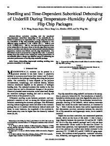
Fig. 11. Bottom scattering strength is shown as a function of bottom arrival angle for data collected in a shallow water environment (77 m). The scattering strength data result from measurements conducted over an area of 0.1 0.08 with flat bathymetry. The error bars represent the standard deviation of individual scattering strength estimates for each angular bin.
2
data that contribute to these estimates are filtered prior to inclusion into the estimates. Filtering is used to eliminate any s that produce “unphysical” point estimates of scattering strength. In addition, a threshold may be applied that requires s for a given grid cell in order to a minimum number of compute scattering strengths. These criteria prevent estimations of scattering strengths from sparsely populated grid cells. Finally, it should be noted that although the above description of scattering strength estimation is presented as a series of successive processes that are applied to the SABLE database, the actual implementation is composed of a single algorithm that operates on the SABLE database. Once the appropriate constraints and user-specified binning resolutions are set, production of the gridded scattering strength database is automated through a single processing routine. As an example of a scattering strength estimate produced by the SABLE process, results from a shallow water measurement are shown in Fig. 11. These results are preliminary, but they serve as an illustration of how SABLE can produce meaningful acoustic estimates, even in very difficult environments. The data used to produce the results in the following discussion consisted of 1110 pings of data collected from the AN/SQS-53C sonar. For each ping, 24 beams of data were processed. The ensonified in an area of flat bathymetry. area covered approximately 5 The nominal water depth in the measurement area was 77 m. Measurements were made at approximately 3500 Hz using a high-bandwidth coded waveform that supported the maximum time scale resolution available in this sonar system. A total of were ob117 771 discrete reverberation measurements s included both direct tained from the sonar data set. These and multibounce eigenpaths. Filtering of the data for only dipoints. Thus, rect-path matched eigenrays yielded 15 378 the eigenray matching/direct-path restrictions eliminated 87% points. With the additional constraints applied of the initial as discussed above, scattering strength versus grazing angle was then computed for the measurement area. The results are presented in Fig. 11. For a given grazing angle, the mean scattering strength and the standard deviation of the estimate are shown. Estimates of scattering strength at higher grazing angles
742
IEEE JOURNAL OF OCEANIC ENGINEERING, VOL. 30, NO. 4, OCTOBER 2005
Fig. 12.
Schematic ray diagram is shown for a traditional geometry used in bottom loss measurements.
Fig. 13.
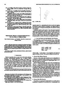
Schematic ray diagram is shown for a monostatic bottom loss geometry.
were possible in this measurement because the sonar depression angle was varied during the course of the measurement to cover a wider range of incident angles and because of the relatively wide vertical beam width of the sonar. It is also significant that the results presented here result from data collected over a range of geometries, locations within the measurement areas, and azimuthal bearings rather than highly constrained geometries often associated with scientific experiments. B. Monostatic Bottom Loss Measurement and Estimation Bottom loss is defined [1] as the ratio of the forward reflected plane wave intensity to the incident plane wave intensity at the seafloor for a particular grazing angle , i.e., (10) Traditional methods for measurements of bottom loss require a bistatic geometry, where the transmitter and receiver are at different locations. A typical geometry is illustrated in Fig. 12. In these measurements, the geometry changes with time as either the source or receiver moves, thus increasing or decreasing the range and decreasing or increasing the grazing angle, respectively. With a monostatic (collocated) source and receiver, as illustrated in Fig. 13, it is not possible to have a forward scatter observable as with a traditional bistatic bottom loss measurement system. Estimates of bottom loss with a monostatic measurement system require a new paradigm.
Consider the propagation along a single eigenray that experiences two bottom bounces, as shown in Fig. 13. The reverberation level due to the scattering at the second bottom bounce at the receiver can be written as (11) is the source level, is the one-way transmission loss (excluding bottom loss), is the bottom loss, is the is the area of ensonification on the scattering strength, and seafloor where factors such as pulse length or sampling window duration are accounted for. With the addition of indices to the notation, it is possible to indicate if a particular term is associated with the source/receiver (remembering they are collocated as shown in Fig. 13), the first bottom bounce, or the second bottom bounce, denoted by subscripts 0, 1, and 2, respectively. Solving for bottom loss yields (12) In case of a monostatic sensor, the observable is the reverber. The system source level is known from ation level design specifications and may be verified through calibration can be estimated as described in the previous tests; the area section; and transmission loss due to geometrical spreading and is obtained from a numerical model (setting attenuation the bottom loss to zero) as described in the previous section. Sonar system parameters such as source level, waveform, and
BROWN AND BARLETT: MIDFREQUENCY “THROUGH-THE-SENSOR” SCATTERING MEASUREMENTS
sampling window characteristics are accounted for as described in previous sections. and ). To solve for In (12), there are two unknowns ( , the scatter strength must be estimated. This may be done by breaking the problem into two steps: solving for in the first in a second pass. This is accomplished in pass and solving for the first pass by creation of a georeferenced scatter strength database as described in the previous section. Since the geographic los are known, a scattering cations of s and corresponding strength may be retrieved from the existingdatabase when solving (12). Of course, this is a very general description of a complicated algorithm. Additional details are developed below. The strategy utilized to make bottom loss estimates relies on , ) pairs, corresponding with and , finding ( respectively, that are associated with the same eigenray. Using parameters in the SABLE database, restrictions on various “associated pairs” of discrete measurements can be identified that can then be used to estimate bottom loss via the two-pass process previously summarized. To perform the search in an acceptable amount of time, an algorithm was developed to sort and match the appropriate database parameters in a sequential series of tests in order to reduce the degrees of freedom. The initial process is to compile and sort all unique values of ping times contained in the database. These results are then written to a file containing the ping times in the SABLE database. For each ping time, all measurements that correspond to either a single bottom bounce or a double bottom bounce propagation path are then identified. Next, filtering is performed on the single and double bottom bounce measurements to identify particular pairs that are associated with the same eigenray for a given ping associated with a double bottom bounce time. For a given eigenpath, corresponding single bounce s( ) that can be associated with the same propagation path are idens are required tified using a series of constraints. First, the to lie along the same bearing from the transmitter as the given . s with common (to a given ) bearings are then required to have a range from the transmitter of of the range, where is a range uncertainty parameter. This constraint arises from a simple range relationship between the first and second bottom bounce distances, assuming flat in, asterfaces and specular reflection. Finally, for a given s are required to have the same eigenray launch sociated . If the resulting filtering angle within a specified variance of data yields more than one for a specific after these tests are applied, then these data are not used in a bottom loss calculation. However, due to time/range (signal spread) and horizontal and vertical angle spread of the propagating wave, is permitted to be associated with a spemore than one . Constraints imposed for quality control in filtering cific , ) and matching result in a reduced population of ( pairs for use in bottom loss estimation compared to the population of data available for scattering strength measurements. , ) pairs and with a georeferWith the matched ( enced scattering strength database to estimate , (12) may now . Moreover, because each has a specific be solved for eigenray associated with it and because it is georeferenced, the seafloor may be gridded to any desired resolution. Thus, it is s for all grazing angles that occur possible to accumulate all
743
Fig. 14. Gridded population map of discrete measurements shown for the monostatic bottom loss example presented in the paper. The gray scale {color} bar shows the logarithmic population [10 log 10(cell population)] scale. A 2-min gridding resolution was used in the analysis. (Color version available online at http://ieeexplore.ieee.org.)
s in in a particular grid cell. The ability to associate many a grid from previously unrelated reverberation curves permits the estimation of bottom loss versus grazing angle for the cell in question. The above algorithm has the ability to produce a bottom loss versus grazing angle curve over the entire range of grazing angles. However, due to operational limitations of the sonar system, most available data sets will have a limited eigenray sonar launch and bottom grazing angle distributions. Applications such as numerical modeling of reverberation may require bottom loss inputs over a wide range of angles or over a range of angles not supported in a particular data set. Therefore, a method is needed to extrapolate bottom loss estimates from the SABLE database over a larger angular space. A variety of approaches are possible for extending bottom loss estimates to larger angular ranges, including various modelbased approaches and inversion techniques. However, to illustrate how bottom loss measurements over limited angular ranges may be extended, a straightforward approach is presented in the following. The Marine Geophysical Survey project [1], [19], which was managed by the Naval Oceanographic Office, obtained bottom loss measurements from a variety of areas worldwide. This project created a set of bottom loss curves for use in the range 1–4 kHz. These bottom loss curves became a standard and are frequently referred to as “MGS curves.” In order to extrapolate SABLE estimates of bottom loss to a broader range of angles, an algorithm was devised to select an MGS curve from a limited set of bottom loss estimates. For each grid cell, the bottom loss measurements are binned at a user-specified resolution and angular range. The mean bottom loss value for each angular bin is then compared to the set of MGS curves to find the curve that most closely agrees with that specific bin. This is repeated for all bins in each grid cell. For each grid cell, a mean MGS value is then computed over the range of angles supported by the bottom loss data. This mean value is rounded to the nearest whole integer, and this becomes the MGS value assigned to that particular grid cell in the georeferenced bottom loss curve database. Of course, georeferenced bottom loss versus grazing angle databases may also be produced in a manner similar to those described for the scattering strength estimates. Results for a bottom loss estimation using a SABLE database and the above method are shown in Figs. 14–18. In Fig. 14, the
744
IEEE JOURNAL OF OCEANIC ENGINEERING, VOL. 30, NO. 4, OCTOBER 2005
Fig. 15. Angular bin population (upper panel) and mean bottom loss estimates as a function of angle (lower panel) are shown for the cell (2,5) [row,column] in Fig. 14. The error bars shown in the lower panel represent the standard deviation of the individual bottom loss estimates for each angular bin. (Color version available online at http://ieeexplore.ieee.org.)
estimated bottom loss versus grazing angle does not clearly delineate a specific MGS curve but rather spans MGS curves 2–4, with the means most closely matching MGS curve 3. The results of Figs. 15 and 16 correspond to grid cell (2,5) [row,column] of Fig. 14. Corresponding results/figures for grid cell (4,4) are shown in Figs. 17 and 18. Again, the statistical uncertainties span several MGS curves, but the mean bottom loss values approximate the values and angular dependence of MGS curve 2. A larger angular range of bottom loss estimates may provide better discrimination between MGS curves, but unfortunately the sonar data may not support extended angular ranges for bottom loss estimates. Refinements of the techniques discussed in this section provide a possible means of reducing bottom loss estimation variance and thus may ultimately provide a more robust means of associating monostatic bottom loss estimates with MGS provinces or other methods of extrapolating angular relationships of bottom loss. Fig. 16. Bottom loss estimates for cell (2,5) are compared with the MGS curves. MGS curves 1–9 are represented by the curves from the top to the bottom of the figure, respectively. (Color version available online at http://ieeexplore.ieee.org.)
population of s that have been matched to a corresponding via the above method is shown for an example SABLE database. The grid cell resolution used in the example is 2 min. The log population density values range from about 15 to 35 for this example. Examples of estimated bottom loss in particular grid cells and the corresponding bottom loss versus MGS curve comparisons are shown in Figs. 15 and 16. The upper panel of Fig. 15 shows the population of grid cell versus grazing angle while the bottom panel shows the mean bottom loss as a function of grazing angle. The error bars shown in the bottom panel represent the standard deviation of the estimates in each angular bin. Angular binning was performed in 2 increments for this example. Fig. 16 shows the corresponding estimated bottom loss versus MGS curve comparison. As seen in the figure, the
VI. DISCUSSION AND SUMMARY In this paper, a new paradigm for “through-the-sensor” remote sensing of the seafloor is presented. The methodology, known as SABLE, is based on beamformed basebanded reverberation data obtained through the AN/SQS-53C sonar, which is found on many U.S. Navy destroyers. The fundamental component of the SABLE paradigm is a georeferenced point database that contains discrete measurements of signal characteristics obtained from the reverberation data as well as associated ship navigation and sonar system parameter information. Environmental (bathymetry and sound speed) information and modeled propagation characteristics are also included for each database point through a data fusion process. The resulting SABLE database can then be used to produce various products. A fundamental design goal of the SABLE project is to not make any special requests of the sonar operator. This design
BROWN AND BARLETT: MIDFREQUENCY “THROUGH-THE-SENSOR” SCATTERING MEASUREMENTS
745
Fig. 17. Angular bin population (upper panel) and mean bottom loss estimates as a function of angle (lower panel) are shown for cell (4,4) [row,column] in Fig. 14. The error bars shown in the lower panel represent the standard deviation of individual bottom loss estimates for each angular bin. (Color version available online at http://ieeexplore.ieee.org.)
Fig. 18. Bottom loss estimates for cell (4,4) are compared with the MGS curves. MGS curves 1–9 are represented by the curves from the top to the bottom of the figure, respectively. (Color version available online at http://ieeexplore.ieee.org.)
goal requires no certain waveforms, sonar modes, or beam coverages, albeit some sonar configurations have advantages in specific ocean acoustic environments. Although the focus of this initial work is on bottom scattering strength and bottom loss, there are no fundamental limitations in technology that prevent investigations of surface or volume scattering phenomena. On the contrary, the addition of these capabilities is planned for future upgrades of SABLE. One of the primary concerns regarding the current extracting of scattering strength and bottom loss is the potential contamination of the data with volume scattering from biological scatterers distributed in the water column. This problem is somewhat mitigated by the fact that the current algorithms discriminate against volume scatterers in favor of bottom
scatterers through depth matching algorithms. These algorithms are not perfect due to the fact that in a multipath environment there are eigenpath and travel time ambiguities. The consistency and repeatability of results from ambiguity resolution algorithms promote a confidence that they are performing reasonably well from a statistical point of view. The reliability of the algorithms to discriminate between volume and bottom scatterers is without question depth dependent. One significant advantage of the approach outlined here is the inherent ability to address these and other issues within a single computational environment developed for this research. Recommendations for future work include development of better algorithms to detect likely volume scattering mechanisms. This may include frequency domain processing and analysis; it may also include time-dependent analysis of scattering from discrete georeferenced patches of the seafloor or other techniques. Additional areas for future investigations include 1) improved extrapolation of both bottom scattering strength and bottom loss to a larger range of arrival angles when the data have limited arrival angles, and 2) implementation of geoacoustic parameter estimation algorithms. The ability to filter or constrain the SABLE database based on various parameters or combinations of parameters is an important feature of this paradigm. Such procedures are typically used to select database points that are appropriate for use in the estimation of specific acoustic parameters and to evaluate and/or control the quality of the data being used in the estimations. The capability to display database parameters as an analysis aid was illustrated. In addition, the generation of gridded statistics and estimates from the point database was discussed and is an important component in processes where acoustic parameters are being estimated. Two examples of how acoustic parameters are estimated from the SABLE database were described. Estimation of scattering parameters relies on the ability to associate specific propagation paths (eigenpaths) in the ocean with discrete measurements in the database. In addition, the estimation process
746
exploits the capability of SABLE to combine independent measurements (made at different times, from different aspects, etc.) at a given geographic location to produce the estimates. In the determination of scattering parameters, SABLE also accounts for sonar system dependencies, such as beam pattern effects, calibration factors, and source levels, that can vary depending on the sonar system settings. Bottom scattering strength was estimated for a data set that was collected in a very shallow water environment. In this example, the ability to resolve discrete propagation paths and associate these with specific discrete reverberation measurements was illustrated. The resulting output from the SABLE processing consisted of a scattering strength versus grazing angle estimate over the measurement area. A second example of monostatic bottom loss estimation was also given. The estimation of monostatic bottom loss required the development of a new paradigm in which the estimation is done using a two-stage process. Critical to this approach is the ability to associate first and second bottom bounce discrete measurements in the database with the same eigenpath. This association is produced using a series of tests and constraints on point data used in the estimates. Once these associations have been completed, bottom loss can then be estimated using scattering strength estimates that are also obtained from the database to eliminate one of the two unknowns in the sonar equation that describes the measurement. Significant progress has been made in developing the capability to make “through-the-sensor” oceanographic measurements via the SABLE paradigm. There are several key components that are necessary to provide this potential. First, in “through the sensor” measurements, it is important not only to obtain the acoustic data but also to have the associated sonar system information as these sensors typically have variable operational features that must be accounted for in order to produce reasonable results. Another key feature of SABLE is the eigenray matching that is part of the SABLE process. Since SABLE relies on discrete acoustic measurements of reverberation as the basis for estimating acoustic scattering parameters, the eigenray matching process is important for identifying discrete measurements that are dominated by the appropriate propagation conditions. This feature greatly reduces the dependency of derived scattering parameters on the underlying sampling scheme that is used to sample the reverberation time series. Finally, for many measurements, the estimation of the ensonified area is also an important component. SABLE uses a relatively simple approximation for the ensonified area. Uncertainties in the ensonified area often directly contribute to variance in scattering parameter estimates. More accurate ways to estimate the ensonified area are under investigation. Improved area estimates should translate directly to more accurate estimates of bottom scattering. Finally, it is worth noting that although the focus of this paper has been on bottom scattering characterizations using the SABLE approach, the SABLE paradigm can also be used in estimates of surface scattering and volume reverberation characterization. By changing the way the SABLE database s that are is constrained/filtered, it is possible to select associated with surface or volume scattering rather than bottom
IEEE JOURNAL OF OCEANIC ENGINEERING, VOL. 30, NO. 4, OCTOBER 2005
interactions. Scattering estimates can then be constructed with an approach similar to those discussed above for bottom scattering. APPENDIX TABLE I IDENTIFICATION AND SONAR PARAMETERS
TABLE II COMPUTED OR DERIVED FROM REPLICA CORRELATED CP WAVEFORM
BROWN AND BARLETT: MIDFREQUENCY “THROUGH-THE-SENSOR” SCATTERING MEASUREMENTS
TABLE III COMPUTED OR DERIVED FROM CP AND CW WAVEFORMS AT BEAMFORMER
TABLE IV ENVIRONMENTAL AND MODELING INPUTS
747
[6] G. M. Anderson, R. T. Miyamoto, M. L. Boyd, and J. I. Olsonbaker, “Sonar environmental parameter estimation system,” Appl. Phys. Lab. Univ. Washington APL:UW, Seattle, WA, Tech. Rep. APL-UW TR 0101, Apr. 2002. [7] M. T. Sundvik, M. T. Rabe, and M. J. Vaccaro, “Mapping seabed acoustic reflection and scattering coefficients using tactical sonar systems,” in Proc. MTS/IEEE OCEANS Conf., Seattle, WA, Sep. 13–16, 1999, pp. 1298–1304. [8] J. L. Bishop, M. T. Sundvik, and D. W. Grande, “Method for real-time extraction of ocean bottom properties,” U.S. Patent 5 475 651, Dec. 12, 1995. [9] J. H. Wilson, S. Rajan, and J. Null, “Inversion techniques and the variability of sound propagation in shallow water,” IEEE J. Ocean. Eng., vol. 21, no. 4, pp. 321–322, Oct. 1996. [10] D. Chandler, Introduction to Modern Statistical Mechanics. Oxford, U.K.: Oxford Univ. Press, 1987. [11] W. E. Brown, M. L. Barlett, and J. F. England, “Construction and visualization of a seafloor backscatter database using “through the sensor” technology,” in Proc. MTS/IEEE OCEANS Conf., Seattle, WA, Sep. 13–16, 1999, pp. 1275–1280. [12] W. E. Brown, D. R. Newcomb, M. L. Barlett, G. H. Rayborn, and F. Bentrem, “Development of multipurpose signal attribute and environmental databases from combatant sensors,” in Proc. MTS/IEEE OCEANS Conf., Honolulu, HI, Nov. 5–8, 2001, pp. 1672–1677. [13] W. E. Brown, M. L. Barlett, and G. H. Rayborn, “Estimation of ocean bottom scattering strength using discrete eigenray matching,” in Proc. MTS/IEEE OCEANS Conf., Honolulu, HI, Nov. 5–8, 2001, pp. 1636–1639. [14] W. E. Brown, M. L. Barlett, and R. L. Dicus, “Impact of windowing and subsampling algorithms on acoustic scattering strength databases,” in Proc. MTS/IEEE OCEANS Conf., Biloxi, MS, Oct. 29–31, 2002, pp. 1258–1263. [15] W. E. Brown, “Remote sensing of the seafloor: A new paradigm,” Ph.D. dissertation, Univ. Southern Mississippi, Hattiesburg, May 2004. [16] K. Grenbowicz and B. Howell, “Quality control of ocean temperature and salinity profile data,” in Proc. MTS/IEEE OCEANS Conf., Biloxi, MS, Oct. 29–31, 2002, pp. 1253–1257. [17] W. Teague, M. J. Carron, and P. J. Hogan, “A comparison between the generalized digital environmental model and levitus climatologies,” J. Geophys. Res., vol. 95, no. C5, pp. 7167–7183, 1990. [18] CASS Reference Guide, Naval Undersea Warfare Center Detachment, New London, CT, Mar. 1994. [19] R. J. Urick, “Sound propagation in the sea,” Defense Advanced Research Projects Agency, 1979.
Walter E. Brown received the B.S. degree in geology from the Mississippi State University, Starkville, MS, in 1975, the M.S. degree in oceanography from The Naval Postgraduate School, Monterey, CA, in 1981, and the Ph.D. degree in scientific computing from The University of Southern Mississippi, Hattiesburg, MS, in 2004. He has worked for government, university, and private industry laboratories in the areas of underwater acoustic modeling, the effects of the propagation media on sensor systems performance, signal processing and classification, nonlinear signal physics, and remote sensing. He is currently with the Naval Oceanographic Office, Stennis Space Center, MS. Dr. Brown is a member of the Marine Technology Society.
REFERENCES [1] R. J. Urick, Principles of Underwater Sound. New York: McGrawHill, 1983. [2] K. V. Mackenzie, “Bottom reverberation for 530- and 1030-cps sound in deep water,” J. Acoust. Soc. Amer., vol. 33, no. 11, pp. 1498–1504, 1961. [3] C. W. Holland, R. Hollett, and L. Troiano, “A measurement technique for bottom scattering in shallow water,” J. Acoust. Soc. Amer., vol. 108, pp. 997–1011, 2000. [4] G. A. Scanlon, “Estimation of bottom scattering strength from measured and modeled AN/SQS-53C reverberation levels,” M.S. thesis, Naval Postgraduate School, Monterey, CA, May 1994. [5] G. Scanlon, R. Bourke, and J. Wilson, “Estimation of bottom scattering strength from measured mid-frequency sonar reverberation levels,” IEEE J. Ocean. Eng., vol. 21, no. 4, pp. 440–451, Oct. 1996.
Martin L. Barlett received the B.S. degree in physics from the Florida Institute of Technology, Melbourne, FL, in 1974 and the Ph.D. degree in physics from The University of Texas at Austin, Austin, TX, in 1980. From 1974 to 1976, he was a Reactor Test Engineer at Newport News Shipbuilding, Newport News, VA. During his graduate studies, he conducted research in medium energy nuclear physics at the Los Alamos Meson Physics Facility, Los Alamos National Laboratory, Los Alamos, NM. Following graduation, he served as a Post-Doc, Research Associate, and Research Scientist at the Physics Department, The University of Texas at Austin, where he conducted medium and high energy physics experiments at Los Alamos and Brookhaven National Laboratories and at Fermi National Accelerator Laboratory. In 1989, he joined the Applied Research Laboratories at The University of Texas at Austin as a Research Scientist. His main research interests include nonlinear signal processing, autonomous classification, “through the sensor” measurements, and remote sensing. Dr. Barlett is a member of the Acoustical Society of America and the Marine Technology Society.