PUSH: a Generalized Operator for the Maximum Vertex ... - Univ Angers

PUSH: a Generalized Operator for the Maximum Vertex Weight Clique Problem Yi Zhou a , Jin-Kao Hao a,b,∗ , Adrien Go¨effon a a LERIA,

Universit´e d’Angers, 2 Boulevard Lavoisier, 49045 Angers, France b Institut

Universitaire de France, Paris, France

European Journal of Operational Research, http://dx.doi.org/10.1016/j.ejor.2016.07.056

Abstract The Maximum Vertex Weight Clique Problem (MVWCP) is an important generalization of the well-known NP-hard Maximum Clique Problem. In this paper, we introduce a generalized move operator called PUSH, which generalizes the conventional ADD and SWAP operators commonly used in the literature and can be integrated in a local search algorithm for MVWCP. The PUSH operator also offers opportunities to define new search operators by considering dedicated candidate push sets. To demonstrate the usefulness of the proposed operator, we implement two simple tabu search algorithms which use PUSH to explore different candidate push sets. The computational results on 142 benchmark instances from different sources (DIMACS, BHOSLIB, and Winner Determination Problem) indicate that these algorithms compete favorably with the leading MVWCP algorithms. Keywords: Local search; Cliques; Tabu search; Heuristics.

1

Introduction

Given an undirected graph G = (V, E, w) with vertex set V and edge set E ⊆ V × V , let w : V → R+ be a weighting function that assigns to each vertex v ∈ V a positive value wv . A clique C ⊆ V of G is a subset of vertices such that its induced subgraph is complete, i.e., every two vertices in C are pairwise adjacent in G (∀u, v ∈ C, (u, v) ∈ E). For a clique C of G, its weight ∗ Corresponding author. Email addresses: [email protected] (Yi Zhou), [email protected] (Jin-Kao Hao), [email protected] (Adrien Go¨effon).

Preprint submitted to Elsevier

7 August 2016

∑

is given by W (C) = v∈C wv . The Maximum Vertex Weight Clique Problem (MVWCP) is to determine a clique C ∗ of maximum vertex weight. MVWCP is an important generalization of the classical Maximum Clique Problem (MCP) [27]. Indeed, when the vertices of V are assigned the unit weight of 1, MVWCP is equivalent to MCP which is to find a clique C ∗ of maximum cardinality. Given that the decision version of MCP is NP-complete [11], the generalized MVWCP problem is at least as difficult as MCP. Consequently solving MVWCP represents an imposing computational challenge in the general case. Note that MVWCP is different from another MCP variant – the Maximum Edge Weight Clique Problem [1,23] where a clique C ∗ of maximum edge weight is sought. Like MCP which has many practical applications, MVWCP can be used to formulate and solve some relevant problems in diverse domains. For example, in computer vision, MVWCP can be used to solve image matching problems [2]. In combinatorial auctions, the Winner Determination Problem can be recast as MVWCP and solved by MVWCP algorithms [28,29]. Given the significance of MVWCP, much effort has been devoted to design various algorithms for solving the problem over the past decades. On the one hand, there are a variety of exact algorithms which aim to find optimal so¨ lutions. For instance, in 2001, Osterg˚ ard [17] presented a branch-and-bound (B&B) algorithm where the vertices are processed according to the order provided by a vertex coloring of the given graph. This MVWCP algorithm is in fact an adaptation of an existing B&B algorithm designed for MCP [18]. In 2004, Kumlander [12] introduced a backtrack tree search algorithm which also relies on a heuristic coloring-based vertex order. In 2006, Warren and Hicks [25] exposed three B&B algorithms which use weighted clique covers to generate upper bounds and branching rules. In 2016, Wu and Hao [29] developed an algorithm which introduces new bounding and branching techniques using specific vertex coloring and sorting. In 2016, Fang et al. [8] presented an algorithm which uses Maximum Satisfiability Reasoning as a bounding technique. On the other hand, local search heuristics constitute another popular approach to find high-quality sub-optimal or optimal solutions in a reasonable computing time. In 1999, Mannino and Stefanutti [15] proposed a tabu search method based on edge projection and augmenting sequence. In 2000, Bomze et al. [4] formulated MVWCP as a continuous problem which is solved by a parallel algorithm using a distributed computational network model. In 2006, Busygin [5] exposed a trust region algorithm. The same year, Singh and Gupta [22] introduced a hybrid method combining genetic algorithm, a greedy search and the exact algorithm of [7]. In 2008, Pullan [20] adapted the Phase Local Search for the classical MCP to MVWCP. In 2012, Wu et al. [26] introduced a tabu search algorithm integrating multiple neighborhoods. In 2013, Benlic and Hao [3] presented the Breakout Local Search algorithm which also 2

explores multiple neighborhoods and applies both directed and random perturbations. Recently in 2016, Wang et al. [24] reformulated MVWCP as a Binary Quadratic Program (BQP) which was solved by a probabilistic tabu search algorithm designed for BQP. As shown in the literature, local search represents the most popular and the dominating approach for solving MVWCP heuristically. Typically, local search heuristics explore the search space by iteratively transforming the incumbent solution into another solution by means of some move (or transformation) operators. Existing heuristic algorithms for MVWCP [3,20,24,26,28] are usually based on two popular move operators for search intensification: (1) ADD which inserts a vertex to the incumbent solution (a feasible clique), and (2) SWAP which exchanges a vertex in the clique against a vertex out of the clique. In studies like [3,26], another operator called DROP was also used, which simply removes a vertex from the current clique. The algorithms using these operators have reported remarkable results on a large range of benchmark problems. Still as we show in this work, the performance of local search algorithms could be further improved by employing more powerful search operators. This work introduces a generalized move operator called PUSH, which inserts one vertex into the clique and removes k ≥ 0 vertices from the clique to maintain the feasibility of the transformed clique. The proposed PUSH operator shares similarities with some restart and perturbation operators used in MCP and MVWCP algorithms like [3,10] and finds its origin in these previous studies. Meanwhile, as we show in this work, the PUSH operator not only generalizes the existing ADD and SWAP operators, but also offers the possibility of defining additional clique transformation operators. Indeed, dedicated local search operators can be obtained by customizing the set of candidate vertices considered by PUSH. Such alternative operators can then be employed in a search algorithm as a means of intensification or diversification. To assess the usefulness of the PUSH operator, we experiment two restart tabu search algorithms (ReTS-I and ReTS-II), which explore different candidate push sets for push operations. ReTS-I operates on the largest possible candidate push set while ReTS-II works with three customized candidate push sets. Both algorithms share a probabilistic restart mechanism. The proposed approach is assessed on three sets of well-known benchmarks (DIMACS, BHOSLIB, and Winner Determination Problem) of a total of 142 instances. The computational results indicate that both ReTS-I and ReTS-II compete favorably with the leading MVWCP algorithms of the literature. Moreover, the generality of the PUSH operator could allow it to be integrated within any local search algorithm to obtain enhanced performances. The paper is organized as follows. Section 2 formally introduces the PUSH operator. Section 3 presents the two push-based tabu search algorithms. Section 3

4 reports our experimental results and comparisons with respect to state-ofthe-art algorithms. Section 5 is dedicated to an experimental analysis of the restart strategy while conclusions and perspectives are given in Section 6.

2

PUSH : a generalized operator for MVWCP

2.1 Preliminary definitions Let G = (V, E, w) be an input graph as defined in the introduction, C ⊆ V a feasible solution (i.e., a clique) such that any two vertices in C are linked by an edge in E (throughout the paper, C is used to designate a clique), and v ∈ V an arbitrary vertex. We introduce the following notations: ¯ (v) denote respectively the set of adjacent and non-adjacent - N (v) and N ¯ (v) = {u : vertices of a vertex v in V , i.e., N (v) = {u : (v, u) ∈ E} and N (v, u) ∈ / E}. ¯C (v) denote respectively the set of adjacent and non-adjacent - NC (v) and N ¯C (v) = C ∩ N ¯ (v). vertices of a vertex v in C, i.e., NC (v) = C ∩ N (v) and N - Ω is the search space including all the cliques of G, i.e., Ω = {C ⊆ V : ∀v, u ∈ C, v ̸= u, (v, u) ∈ E}. - m is a move operator which transforms a clique to another one. We use C ⊕ m to designate the clique C ′ = C ⊕ m obtained by applying the move operator m to C. C ′ is called a neighbor solution (or neighbor clique) of C. - Nm is the set of neighbor solutions that can be obtained by applying m to an incumbent solution C. ∑

The weight W (C) = v∈C wv of a solution (clique) C ∈ Ω is used to measure its quality (fitness). For two solutions C and C ′ in Ω, C ′ is said to be better than C if W (C ′ ) > W (C). The weight W (C ∗ ) of the best solution ever found by a search procedure is abbreviated as W ∗ . 2.2 Motivations for the PUSH operator

As shown in the literature, local search is the dominating approach for tackling MVWCP (see for example, [3,20,26,28]). Local search typically explores the search space by iteratively transforming an incumbent solution C to a neighbor solution (often of better quality) by means of the following move operators: • ADD extends C with a vertex v ∈ V \ C which is necessarily adjacent to all the vertices in C. Each application of ADD always increases the weight of C and leads to a better solution. 4

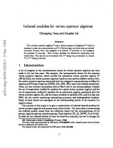
• SWAP exchanges a vertex v ∈ V \ C with another vertex v ′ ∈ C, v being necessarily adjacent to all vertices in C except v ′ . Each application of SWAP can increase the weight of C (if wv > wv′ ), keep its weight unchanged (if wv = wv′ ) or decrease the quality of C (if wv < wv′ ). In some cases like [3,26], a third move operator (DROP ) was also employed which simply removes a vertex from C (thus always leading to a worse neighbor solution). Generally, local search for MVWCP aims to reach solutions of increasing quality by iteratively moving from the incumbent solution to a neighbor solution. This is typically achieved by applying ADD whenever it is possible to increase the weight of the clique, applying SWAP when no vertex can be added to the clique and occasionally calling for DROP to escape local optima. However, as both ADD and SWAP have a prerequisite on the operating vertex in V \ C, these operators may miss improving solutions in some cases. To illustrate this point, we consider the example of Fig. 1 where vertex weights are indicated in brackets next to the vertex labels. As shown in Fig. 1(a), C = {a, b, c} is a clique with a total weight of 12. Since vertex d is neither adjacent to a nor b, d cannot join clique C by means of the ADD and SWAP operators. Meanwhile, one observes that if we insert vertex d into the clique and remove both vertices a and b, we obtain a new clique C ′ (Fig. 1(b)) of weight of 13, which is better than C. Inspired by this observation, the PUSH operator proposed in this work basically transforms C by pushing a vertex v taken from a dedicated subset of V \ C into C and removing, if needed, one or more vertices from C to reestablish solution feasibility. Indeed, when the added vertex v is not adjacent to all the vertices in C, the vertices of C which are not adjacent to v (i.e., the ¯C (v) as defined in Section 2.1) need to be removed from vertices in the set N C to maintain the feasibility of the new solution. In the above example, C can be transformed to a better solution by pushing vertex d into the clique and then expelling both a and b.

2.3 Definition of the PUSH Operator

Let C be a clique, and v an arbitrary vertex which does not belong to C (v ∈ V \ C). P U SH(v, C) (or P U SH(v) for short if the current clique does not need to be explicitly emphasized) generates a new clique by first inserting v into C and then removing any vertex u ∈ C such that (u, v) ∈ / E (i.e., ¯C (v), see Section 2.1). u∈N Formally, the neighbor clique C ′ after applying P U SH(v) (v ∈ V \ C) to C 5

(b)

(a)

Fig. 1. An example which shows that a better solution can be reached by the PUSH operator, but cannot be attained by the traditional ADD and SW AP operators.

is given by: ¯C (v) ∪ {v} C ′ = C ⊕ P U SH(v) = C \ N Consequently, the set of neighbor cliques induced by P U SH(v) in the general case, denoted by NP U SH is given by: NP U SH =

∪

{C ⊕ P U SH(v)}

(1)

v∈V \C

For each neighbor solution C ′ = C ⊕ P U SH(v) generated by a P U SH(v, C) move, we define the move gain (denoted by δv ) as the variation in the objective function value between C ′ and C: δv = W (C ′ ) − W (C) = wv −

∑

wu

(2)

¯C (v) u∈N

Thus, a positive (negative) move gain indicates a better (worse) neighbor solution C ′ compared to C while the zero move gain corresponds to a neighbor solution of equal quality. Typically, a local search algorithm makes its decision of moving from the incumbent solution to a neighbor solution based on the move gain information at each iteration. In order to be able to efficiently compute the move gains of neighbor solutions, we present in Section 3.5 fast streamlining evaluation techniques with the help of dedicated data structures. One notices that PUSH shares similarities with some customized restart or perturbation operators used in [3,10] and finds its origin in these previous studies. In the iterated local search algorithm designed for MCP by Grosso et al. [10], the clique delivered at the end of each local optimization stage is perturbed by insertion of a random vertex and serves then as a new starting 6

point for the next stage of local optimization. In the BLS algorithm for MCP and MVWCP presented by Benlic and Hao [3], each random perturbation adds a vertex such that the resulting clique must satisfy a quality threshold. In these two previous studies, clique feasibility is established by a repair process which removes some vertices after each vertex insertion.

2.4 Special cases of PUSH

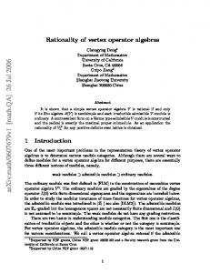
From the general definition of PUSH given in the last section, we can customize the move operator by identifying a dedicated vertex subset of V \ C called candidate push set (CPS) that provides the candidate vertices for PUSH. We first discuss two special cases by considering non-adjacency information ¯C (v) (see the notations introduced in Section 2.1). convoyed by N ¯C (v)| = 0, v ∈ V \ C}, then PUSH is - If CPS is given by A = {v : |N equivalent to ADD. ¯C (v)| = 1, v ∈ V \ C}, then PUSH is - If CPS is given by B = {v : |N equivalent to SWAP. We can also use other information like move gain to constrain the candidate push set, as illustrated by the following examples. (1) If CPS is given by M1 = {v : δv > 0, v ∈ V \ C}, then PUSH always leads to a neighbor solution better than C. ¯C (v)| = 1, v ∈ V \ C}, then PUSH (2) If CPS is given by M2 = {v : δv ≤ 0, |N exchanges one vertex in V \ C with one vertex in C, leading to a solution of equal or worse quality relative to C. ¯C (v)| > 1, v ∈ V \ C}, then (3) If CPS is given by M3 = {v : δv ≤ 0, |N PUSH inserts one vertex into C and removes at least two vertices from C, leading to a solution of equal or worse quality relative to C. (4) If CPS is given by V \ C, then the candidate push set is not constrained. One notices that V \ C = M1 ∪ M2 ∪ M3 . An example of these special cases is provided in Fig. 2. In addition to the ADD and SWAP operators, several restart rules of local search algorithms for MCP can also be recast with the PUSH operator. In particular, the restart Rule 1 in [10] (previously used in [19]) states that C := [C ∩ N (v)] ∪ {v}, v picked at random in V \ C (i.e., add a random vertex v in the clique while keeping in the clique the adjacent vertices of v). This rule is equivalent to push a vertex from candidate push set V \ C into the current solution. As to the restart Rule 2 in [10], let us define the candidate push set Sq = {v : δv ≤ 1 − q, v ∈ V \ C} (q > 0 is a fixed parameter). Then the Rule 2 is to push a random vertex from Sq into C if Sq is not empty; otherwise, 7

Fig. 2. A simple graph labeled with vertex weights in brackets. The current clique ¯C (e) = ∅, N ¯C (f ) = {a}, is C = {a, b, c, d}, W (C) = 2 + 3 + 4 + 5 = 14, N ¯C (g) = {a, b}, N ¯C (h) = {c, d}, N ¯C (i) = {a, b, c}, thus, δe = 2, δf = 0, δg = 1, N δh = −1, δi = −3. According to the definitions, A = {e}, B = {f }, M1 = {e, g}, M2 = {f }, M3 = {h, i}.

push a random vertex from V \ C. Moreover, in the BLS algorithm for MCP and MVWCP [3], the so-called random perturbation modifies the incumbent clique by adding vertices such that the quality of the resulting clique is not deteriorated more than a quality threshold. This random perturbation strategy can simply be considered as applying the PUSH operator to vertices from the candidate push set M4 = {v : δv > (α−1)∗W (C), v ∈ V \C} (where 0 < α < 1 is a predefined parameter). Finally, by considering other candidate push sets subject to specific conditions, it is possible to obtain multiple customized search operators that can be employed by any local optimization procedure to effectively explore the search space. In the next section, we present two local search algorithms based on the above M1 , M2 , M3 and V \ C candidate push sets.

3

PUSH-based tabu search

In this section, we introduce two simple Restart Tabu Search [9] algorithms (denoted by ReTS-I and ReTS-II). Both algorithms rely on the PUSH operator, but explore different candidate push sets. In ReTS-I, the candidate push set considered includes all the vertices out of the clique (i.e., CPS = V \ C) while in ReTS-II, the algorithm jointly considers the candidate push sets M1 , M2 and M3 introduced in Section 2.3. 8

Both ReTS-I and ReTS-II share the same restart local search framework as shown in Algorithm 1, but implement different local optimization procedures with different CPS (line 5, see Sections 3.3 and 3.4). The general framework starts from an initial solution C (or initial clique) generated by means of Random Solution (Section 3.1). The solution is then improved by one of the dedicated tabu search procedures described respectively in Sections 3.3 and 3.4. When the search stagnates in a deep local optimum, the search restarts from a new solution, which is constructed either by Reconstruct Solution (Section 3.2) with probability ρ ∈ [0.0, 1.0] (a parameter), or by Random Solution (Section 3.1) with probability 1 − ρ. It is noted that Reconstruct Solution reconstructs a new solution from C, while Random Solution randomly generates a new solution from scratch. The whole search process repeats the above procedure until a prefixed stopping condition is met. The details of the tabu search optimization procedures and restart procedures are described in the following sections.

1 2 3 4 5 6 7 8 9 10 11

Algorithm 1: Framework of the Restart Tabu Search algorithms for MVWCP Input: G = (V, E, w) - MVWCP instance, ρ - restart probability parameter, L - maximum number of consecutive non-improving iterations. Output: C ∗ - maximum vertex weight clique. begin C∗ ← ∅ ; /* C ∗ maintains the best solution found so far */ C ← Random Solution(G); /* Section 3.1. C is the current solution */ while stopping condition is not met do (C, C ∗ ) ← T abu Search(G, C, C ∗ , L); /* Sections 3.3 and 3.4 */ if random number ∈ [0, 1] < ρ then C ← Reconstruct Solution(G, C) ; /* Section 3.2 */ else C ← Random Solution(G);

/* Section 3.1 */

end return C ∗

3.1 Random initial solution

The Random Solution(G) procedure (Alg. 1, lines 3 and 9) starts from an initial clique C composed by an unique random vertex. Then iteratively, a ¯C (v)| = 0, v ∈ V \ C} (Sections vertex v in candidate push set A = {v : |N 2.3 and 2.4) is randomly selected and added into C. A is then updated by ¯A (v)). The procedure continues until the candidate push A ← A \ ({v} ∪ N ¯C (v)| > 0) is set A becomes empty. A maximal clique (i.e., ∀v ∈ V \ C, |N then reached and returned as the initial solution of the search procedure. This initialization procedure ignores the solution quality (the clique weight), but 9

ensures a good randomness of the initial solutions generated. Such a feature represents a simple and useful diversification technique which helps the search algorithm to start the search in a different region of each repeated run. The initialization procedure can be efficiently implemented with a time complexity of O(|V ||E|). This process is similar to the initial constructive phase preceding the first SWAP move in the MCP algorithm of [10] and also applied in the MVWCP algorithms of [3,26]. 3.2 Solution reconstruction

The reconstruction procedure (Alg. 1, line 7) generates a new solution by iteratively replacing vertices of a given solution. At the beginning, considering a clique C, all the vertices of V \ C are marked available to join C by means of the PUSH operator. Then, at each iteration, the available vertex belonging to candidate push set M1 (see Section 2.4) with the maximum δ value (ties are broken randomly) is selected and pushed into C. Vertices which are removed from C during the PUSH operation are then marked unavailable. As a consequence, they cannot rejoin the solution during the remaining iterations. The reconstruction procedure stops after |C| iterations or when no available vertex may be found from M1 . The current clique C is then returned as the reconstructed solution. Such a reconstruction procedure perturbs the given solution C but, in most cases, does not decrease the quality heavily. The time ¯ (v)|})2 ) as it complexity of each iteration is bounded by O(|V | + (maxv∈V {|N scans the M1 set and calls the PUSH operator (The time complexity of the push operator is discussed in Section 3.5). This reconstruction procedure can also be viewed as an objective-guided strong perturbation procedure since the vertices in the original solution are totally replaced and vertex insertions are subject to the stipulation of the maximum δ value. 3.3 ReTS-I: Tabu search with the largest candidate push set

The first tabu search procedure denoted by ReTS-I uses a greedy rule which gives preference, at each step of the search, to neighbor solutions having the best objective value. ReTS-I implements this heuristic with the largest possible candidate push set V \C. To prevent the search from falling into cycles, a tabu mechanism [9] is incorporated. The general process of ReTS-I is shown in Algorithm 2, where each element tabuv of vector tabu (called the tabu list) records the earliest iteration number that vertex v is allowed to move inside C. At each iteration, one vertex is allowed to join the current solution only when it is not forbidden by the tabu list. Nevertheless, a move leading to a solution better than the best solution 10

found so far is always accepted (this is the so-called aspiration criterion, line 7, Alg. 2). If v is the vertex to be pushed into C, then all the vertices moving ¯C (v)) are forbidden to rejoin the solution for the out of C (i.e., those of N next tt(v) (tabu tenure) iterations (lines 9-10, Alg. 2). The TS procedure ends when the best solution cannot be improved for L (a parameter) consecutive iterations. Note that similar strategies which temporarily forbid the removed vertices to rejoin the solution have been used in [3,10,20,26]. Also note that the added vertex is free to leave the clique. This rule is based on the fact that due to the objective of maximizing the clique weight, an added vertex has little chance to be removed anyway. The tabu tenure tt(v) for a vertex v is empirically fixed as follows: tt(v) = 7 + random(0, η(v))

(3)

¯C (u) = N ¯C (v)}| is the number of vertices which where η(v) = |{u ∈ V \ C : N have as many non-adjacent vertices in C as v, and random(0, n) returns a random integer in range [0, n). Since ReTS-I needs to scan V \ C at each iteration (line 6, Alg. 2), the time complexity of each iteration of ReST-I is bounded by O(|V |). The ReTS-I algorithm is quite simple, but performs well as shown by the experimental outcomes presented in Section 4.

3.4 ReTS-II: Tabu search with three decomposed candidate push sets

Contrary to ReTS-I which explores the whole and unique candidate push set V \ C, ReTS-II, as shown in Algorithm 3, considers more features of the candidate vertices for PUSH. For this algorithm, we decompose V \ C into three candidate push sets M1 , M2 and M3 as defined in Section 2.4. At each iteration, the three CPS are evaluated in a fixed order: M1 → M2 → M3 (lines 7-15) and a vertex with the largest δ value is chosen by PUSH to perform the move. Note that M1 contains preferable vertices as they necessarily increase the weight of the incumbent clique. If no candidate vertex is available in M1 , selecting a vertex from M2 or M3 will degrade the solution (or keep the solution unchanged). Pushing these vertices may be useful to help the search to leave the current local optimum. M2 is evaluated before M3 since pushing a vertex from M2 will generally lead to less vertices to be removed from C than pushing a vertex from M3 . The motivation of using these three sets with a preference order is thus to keep the improvement possibilities as much as possible and proceed to more important perturbations only when no other alternative is possible. 11

1 2 3 4 5 6 7

Algorithm 2: ReTS-I: Tabu search with the largest candidate push set Input: C - current solution, C ∗ - best solution ever found, L - maximum number of consecutive non-improving iterations. Output: C - renewed current solution, C ∗ - maximum vertex weight clique. begin Iter ← 0 ; /* Counter of iterations */ for each v ∈ V do tabuv ← 0 ; /* tabuv is the earliest iteration vertex v is allowed to join C */ l←0; /* Counter of consecutive iterations where C ∗ is not improved */ while l < L do M ← {v ∈ V \ C, tabuv ≤ Iter or W (C) + δv > W (C ∗ )} ; /* M is the set of eligible vertices for PUSH */

8 9 10 11 12 13 14

v ← argmaxv∈M δv ; for u ∈ C \ NC (v) do tabuu ← Iter + tt(v) C ← C ⊕ P U SH(v); if W (C) > W (C ∗ ) then C ∗ ← C; l ← 0;

16

else l ← l + 1;

17

Iter ← Iter + 1;

15

18 19

end return C, C ∗ Moreover, when M3 is used, only a random sample (of a predetermined size r) of vertices in M3 are evaluated for each P U SH operation if no appropriate vertex is found in M1 and M2 . Also, let us precise that PUSH selects the vertex with the best δ value in the sample set. This sampling strategy and its variants were previously used in several studies (ID-Walk [16], Candidate List [9], Best from Multiple Choices [6]). This strategy is obviously more cost effective than evaluating an entire candidate set. ReTS-II uses the same tabu mechanism as ReTS-I. Note that the aspiration criterion does not need to be considered for pushing a vertex from M2 and M3 as better solutions cannot be reached in these cases. Vertices dropped from C by applying PUSH to M2 or M3 are forbidden to rejoin C for consecutive tt(v) iterations (lines 18-19, Alg. 3). The tabu tenure tt(v) is tuned in the same way as in ReTS-I (Section 3.3). Finally, it is interesting to contrast ReTS-I and ReTS-II. In fact, like ReTS-I, ReTS-II also gives priority to candidate vertices leading to a solution of better quality. Meanwhile, when no such kind of vertex exists, ReTS-II may choose a 12

different vertex for the PUSH operation. For example, suppose that the same candidate push set M = {a, b} is applied in Algorithms 2 and 3 with δa = −1, ¯C (a)| = 2, |N ¯C (b)| = 1. Then ReTS-I chooses vertex a while δb = −3, |N ReTS-II selects vertex b for the PUSH operation. Therefore, by using different candidate push sets, ReTS-I and ReTS-II visit different search trajectories to explore the search space. The computational experiments shown in Section 4 will allow us to observe the relative performances of both algorithms.

1 2 3 4 5 6 7 8 9 10 11 12 13

Algorithm 3: ReTS-II: Tabu search with three candidate push sets Input: C - current solution, C ∗ - best solution ever found, L - maximum number of consecutive non-improving iterations, r - maximum sample size of M3 . Output: C - renewed current solution, C ∗ - maximum vertex weight clique found. begin Iter ← 0; for each v ∈ V do tabuv ← 0; l ← 0; while l < L do M ← {v ∈ V \ C, W (C) + δv > W (C ∗ )}; if M ̸= ∅ then l←0;

/* New best solution */

else M ← {v ∈ V \ C, δv > 0 and tabuv ≤ Iter} ; /* Restricted M1 */ if M = ∅ then ¯C (v)| = 1 and tabuv ≤ Iter} ; M ← {v ∈ V \ C, δv ≤ 0 and |N /* Restricted M2 */

14 15

16 17 18 19

if M = ∅ then M ← Randomly sample r vertices from {v ∈ V \ C, tabuv ≤ Iter} ; /* Restricted M3 */ l ← l + 1; Randomly select v ∈ argmaxv∈M δv ; for each u ∈ C \ NC (v) do tabuu ← tt(u)

22

C ← C ⊕ P U SH(v); if l = 0 then C ∗ ← C;

23

Iter ← Iter + 1;

20 21

24 25

end return C, C ∗

13

3.5 Fast evaluation of move gains

As presented in Section 2.3, each neighbor solution relative to a current clique leads to a move gain δ, which can be positive, null or negative. Since move gain evaluations are frequent in the TS procedures, we elaborate a fast streamlining technique which enables a direct access to all possible δ values (i.e., corresponding to the insertion in the current clique of each candidate vertex), as well as a fast update of the impacted move gains at each iteration. In this section, we present this incremental evaluation mechanism. Let us consider a vector ∆ = (δv )v∈V such that δv represents the move gain W (C ⊕ P ush(v)) − W (C). According to the definition in Section 2.3, a PUSH operation is composed of two basic operations: adding a vertex to the current clique C (ADD), and possibly removing one or several vertices from C (DROP ). Pushing a vertex v into a clique C can be viewed as adding v in C before removing from C every vertex which is not adjacent to v. Nevertheless this decomposition implies to consider infeasible solutions between vertex insertion and removals. We propose then to update incrementally ∆ after each basic operation (ADD, DROP ) by first removing from C the vertices which are not adjacent to the pushed vertex v, and finally adding v to C. If a vertex v ′ is removed (dropped) from the current solution C, then the move gain δu of any vertex u ∈ V is updated as follows:    ¯ (v ′ )  δu + wv′ , if u ∈ N   

∀u ∈ V, δu ←  wu      δu

, if u = v ′

(4)

, otherwise

¯ of To speed up the update process, we use the complementary graph G ¯ the input graph G, so that N (v) sets can be explicitly defined. Since only ¯ (v ′ ) ∪ {v ′ } need to be updated, the move gains associated to vertices of N the time complexity of updating ∆ after a DROP operation is bounded by ¯ (v)|}). O(maxv∈V {|N Similarly, when a vertex v is added into the current solution C, then ∆ is updated as follows:    ¯   δu − wv , if u ∈ N (v) δu ←

 

0       δu

, if u = v

(5)

, otherwise

¯ (v)|}). This operation is obviously also bounded in time by O(maxv∈V {|N 14

Thus updating the move gains after a PUSH operation can be performed ¯ (v)|})2 ), since operation C ⊕ P ush(v) involves one ADD in O((maxv∈V {|N ¯C (v)| DROP operations, with |N ¯C (v)| being bounded by operation and |N ¯ (v)|}. maxv∈V {|N

4

Computational experiments

This section is dedicated to an experimental assessment of the two tabu search algorithms using the generalized PUSH operator. The assessment was based on three sets of 142 well-known benchmark instances and comparisons with state-of-the-art MVWCP algorithms.

4.1 Benchmarks

The three benchmark sets include the following instances: 80 DIMACS instances, 40 BHOSLIB instances, and 22 instances from the Winner Determination Problem in combinatorial auctions. • DIMACS benchmarks. This set of 80 instances originated from the second DIMACS implementation challenge for the maximum clique problem 1 . These instances cover both real world problems (coding theory, fault diagnosis, Steiner Triple Problem...) and random graphs. They include small graphs (50 vertices and 1,000 edges) to large graphs (4,000 vertices and 5,000,000 edges). Though DIMACS graphs were originally collected for benchmarking MCP algorithms, these graphs are still very popular and widely used as a testbed for evaluating MVWCP algorithms [3,8,15,20,24,26]. Considering that vertices are unweighted in these instances, we assign to each vertex i (i is an index number) the weight i mod 200 + 1, following the rule in [20]. • BHOSLIB benchmarks. The BHOSLIB (Benchmarks with Hidden Optimum Solutions) instances were generated randomly in the SAT phase transition area according to the model RB 2 . The 40 instances included in this set were widely used to test MCP and MVWCP algorithms. The sizes of these instances range from 450 vertices and 17,794 edges, to 1,534 vertices and 127,011 edges. The weight of each vertex is assigned following the aforementioned rule, i.e., i mod 200 + 1 for vertex i. • Winner Determination Problem (WDP) benchmarks. The Winner Determination Problem can be reformulated as a MVWCP and thus solved 1 2

http://www.cs.hbg.psu.edu/txn131/clique.html http://www.nlsde.buaa.edu.cn/~kexu/benchmarks/graph-benchmarks.htm

15

by MVWCP solvers [28,29]. Therefore, benchmark instances for WDP can also be used to test the performance of MVWCP solvers. Three sets of a total number of 530 instances were reported in [28,29], from which we selected 22 representative instances 3 . Six in instances, whose number of vertices varies among 1,000, 1,500 and 2,000, come from [13]; Ten Decay, Random, Uniform and Wrandom instances are obtained from a generator [21]; P aths and Regions instances are generated using the Combinatorial Auction Test Suite (CATS, [14]). Contrary to the DIMACS and BHOSLIB instances which are defined using integer weights, WDP weights are fractional.

4.2 Experimental protocol

As shown in Algorithms 1 to 3, ReTS-I and ReTS-II share two common parameters: the probability parameter ρ which controls the two types of restart, and the maximum number L of consecutive non-improving iterations before a restart. Besides, ReTS-II has one additional parameter which is the sample size r. For our experiments, we used the following default values: L = 4, 000, r = 50, and ρ = 0.7. We provide an analysis of ρ in Section 5. In general, we observed that varying the parameter values around the default values did not alter much the computational outcomes for most of the tested instances even if some results can be further improved by fine-tuning the parameters. ReTS-I and ReTS-II were coded in C++ 4 and compiled with g++ 4.4.7 with optimization flag -o3. Our experiments were performed on a computer with an AMD Opteron 4184 processor (2.8GHz and 2GB RAM) running Linux 2.6.32. When solving the DIMACS machine benchmarks 5 without compilation optimization flag, the run time on our machine is 0.40, 2.50 and 9.55 seconds respectively for instances r300.5, r400.5 and r500.5. Following the literature [3,24,26], both algorithms were run 100 times to solve each benchmark instance. For the DIMACS and BHOSLIB instances, a maximum of 108 iterations were allowed per run while for the WDP instances, the stopping condition was set to be a cutoff time limit of 10 minutes per run. As discussed in Section 4.4, these settings correspond to the computational effort used by the state-of-the-art MVWCP algorithms in the literature.

3

www.info.univ-angers.fr/pub/hao/wdp.html Our source code will be available at: www.info.univ-angers.fr/pub/hao/ReTS.html. 5 dfmax:ftp://dimacs.rutgers.edu/pub/dsj/clique/ 4

16

4.3 Computational results

Tables 1 to 3 report the computational results obtained by ReTS-I and ReTSII on the DIMACS, BHOSLIB and WDP instances respectively. In these tables, column BKV reports the best-known objective values (BKV) ever found by the previous algorithms [3,8,20,24,26] (proven optima are indicated with the star symbol ’*’ with the BKV values). For each algorithm, column best(hit) indicates the best objective value W ∗ found by ReTS-I and ReTS-II among 100 trials as well as the number of trails hitting the best value (success rate); column ave(std) denotes the average value and the standard deviation of the 100 W ∗ values; column time gives the average seconds of the trails hitting the W ∗ value. The value of 0.00 in columns time indicates that the corresponding average time in seconds is inferior to 0.005. Table 1 discloses that ReTS-I and ReTS-II reach all the best-known results of DIMACS instances except MANN a45 and MANN a81 (indicated in italic), which are believed to be quite challenging for heuristic algorithms [8]. Moreover, for 73 out of 80 instances (> 91%), both algorithms attain the bestknown results in every single trial. For the remaining 7 instances except MANN a45 and MANN a81, each algorithm still hits the best-known results in more than 30 trials. In terms of computational time, most of these instances are solved in less than 1 second. For the 3 hard MANN instances (MANN a27, MANN a45, MANN a81), results are attained in 1 to 17 minutes. From Table 2 on the BHOSLIB instances, one finds that ReTS-I and ReTSII improve the best-known result of the literature on frb53-24-3 (from 5,640 to 5,655). Although both algorithms attain the best-known solutions on 38 out of 40 instances, each algorithm fails to do so in 2 cases (frb50-23-4 and frb56-25-5 for ReTS-I, frb56-23-3 and frb 56-23-4 for ReTS-II, indicated in italic). Interestingly, both algorithms achieve a success rate of at least 93% on the first 20 instances while the success rate drops to less than 50% on most of the last 20 instances. Concerning the computational time, both algorithms require more time to find the best-known solutions when the sizes of the graphs increase, but each average time is inferior to 12 minutes. In general, BHOSLIB instances are more difficult than DIMACS ones for ReTS-I and ReTS-II, but both algorithms still perform quite well by attaining together all the best-known results and finding even an improved best-known result (new best lower bound). Table 3 (WDP instances) shows that ReTS-I and ReTS-II attain the bestknown solutions on all WDP instances considered except the 4 Decay instances and Paths2000 100 (in italic); for Paths2000 100, the algorithms have a success rate of 88% and 76% respectively, while this rate drops to 10% or less for the 4 Decay instances, confirming that these Decay instances are particularly 17

Table 1 Computational results of ReTS-I and ReTS-II on 80 DIMACS instances. instance

BKV

C1000.9 C125.9 C2000.5 C2000.9 C250.9 C4000.5 C500.9 DSJC1000 5 DSJC500 5 MANN a27 MANN a45 MANN a81 MANN a9 brock200 1 brock200 2 brock200 3 brock200 4 brock400 1 brock400 2 brock400 3 brock400 4 brock800 1 brock800 2 brock800 3 brock800 4 c-fat200-1 c-fat200-2 c-fat200-5 c-fat500-1 c-fat500-10 c-fat500-2 c-fat500-5 gen200 p0.9 44 gen200 p0.9 55 gen400 p0.9 55 gen400 p0.9 65 gen400 p0.9 75 hamming10-2 hamming10-4 hamming6-2 hamming6-4 hamming8-2 hamming8-4 johnson16-2-4 johnson32-2-4 johnson8-2-4 johnson8-4-4 keller4 keller5 keller6 p hat1000-1 p hat1000-2 p hat1000-3 p hat1500-1 p hat1500-2 p hat1500-3 p hat300-1 p hat300-2 p hat300-3 p hat500-1 p hat500-2 p hat500-3 p hat700-1 p hat700-2 p hat700-3 san1000 san200 0.7 1 san200 0.7 2 san200 0.9 1 san200 0.9 2 san200 0.9 3 san400 0.5 1 san400 0.7 1 san400 0.7 2 san400 0.7 3 san400 0.9 1 sanr200 0.7 sanr200 0.9 sanr400 0.5 sanr400 0.7

9254 2529 2466 10999 5092* 2792 6955 2186* 1725* 12283* 34265* 111386 372 2821 1428 2062 2107 3422* 3350* 3471* 3626* 3121* 3043* 3076* 2971* 1284 2411 5887 1354 11586 2628 5841 5043* 5416* 6718 6940 8006* 50512* 5129 1072 134 10976 1472 548 2033* 66 511 1153 3317 8062 1514* 5777* 8111 1619* 7360 10321 1057 2487 3774 1231* 3920* 5375* 1441* 5290* 7565 1716* 3370 2422* 6825* 6082* 4748* 1455 3941* 3110* 2771* 9776* 2325* 5126* 1835* 2992*

best(hit) 9254(100) 2529(100) 2466(100) 10999(92) 5092(100) 2792(100) 6955(100) 2186(100) 1725(100) 12283(78) 34259 (1) 111370 (1) 372(100) 2821(100) 1428(100) 2062(100) 2107(100) 3422(100) 3350(100) 3471(100) 3626(100) 3121(100) 3043(100) 3076(100) 2971(31) 1284(100) 2411(100) 5887(100) 1354(100) 11586(100) 2628(100) 5841(100) 5043(100) 5416(100) 6718(100) 6940(100) 8006(100) 50512(100) 5129(100) 1072(100) 134(100) 10976(100) 1472(100) 548(100) 2033(100) 66(100) 511(100) 1153(100) 3317(100) 8062(100) 1514(100) 5777(100) 8111(100) 1619(100) 7360(100) 10321(100) 1057(100) 2487(100) 3774(100) 1231(100) 3920(100) 5375(100) 1441(100) 5290(100) 7565(100) 1716(100) 3370(100) 2422(100) 6825(100) 6082(100) 4748(100) 1455(100) 3941(97) 3110(97) 2771(100) 9776(100) 2325(100) 5126(100) 1835(100) 2992(100)

ReTS-I ave(std) 9254.00(0.00) 2529.00(0.00) 2466.00(0.00) 10996.44(8.72) 5092.00(0.00) 2792.00(0.00) 6955.00(0.00) 2186.00(0.00) 1725.00(0.00) 12282.78(0.41) 34253.60(1.11) 111351.19(6.63) 372.00(0.00) 2821.00(0.00) 1428.00(0.00) 2062.00(0.00) 2107.00(0.00) 3422.00(0.00) 3350.00(0.00) 3471.00(0.00) 3626.00(0.00) 3121.00(0.00) 3043.00(0.00) 3076.00(0.00) 2970.31(0.46) 1284.00(0.00) 2411.00(0.00) 5887.00(0.00) 1354.00(0.00) 11586.00(0.00) 2628.00(0.00) 5841.00(0.00) 5043.00(0.00) 5416.00(0.00) 6718.00(0.00) 6940.00(0.00) 8006.00(0.00) 50512.00(0.00) 5129.00(0.00) 1072.00(0.00) 134.00(0.00) 10976.00(0.00) 1472.00(0.00) 548.00(0.00) 2033.00(0.00) 66.00(0.00) 511.00(0.00) 1153.00(0.00) 3317.00(0.00) 8062.00(0.00) 1514.00(0.00) 5777.00(0.00) 8111.00(0.00) 1619.00(0.00) 7360.00(0.00) 10321.00(0.00) 1057.00(0.00) 2487.00(0.00) 3774.00(0.00) 1231.00(0.00) 3920.00(0.00) 5375.00(0.00) 1441.00(0.00) 5290.00(0.00) 7565.00(0.00) 1716.00(0.00) 3370.00(0.00) 2422.00(0.00) 6825.00(0.00) 6082.00(0.00) 4748.00(0.00) 1455.00(0.00) 3932.00(51.18) 3105.26(26.95) 2771.00(0.00) 9776.00(0.00) 2325.00(0.00) 5126.00(0.00) 18 1835.00(0.00) 2992.00(0.00)

time 2.50 0.00 2.34 417.56 0.01 116.05 0.06 0.38 0.13 82.77 157.98 990.02 0.00 0.00 0.00 0.00 0.00 0.04 0.04 0.07 2.04 0.14 0.39 0.39 835.03 0.00 0.00 0.00 0.01 0.11 0.02 0.09 0.00 0.12 0.18 0.05 0.03 0.20 26.25 0.00 0.00 0.01 0.00 0.00 0.04 0.00 0.00 0.00 1.12 532.74 0.14 0.11 0.19 0.32 0.35 2.06 0.00 0.01 0.01 0.03 0.02 0.04 0.04 0.06 0.10 71.07 0.21 0.04 0.04 0.00 0.01 0.19 172.04 234.69 0.41 2.38 0.00 0.00 0.02 0.03

best(hit) 9254(100) 2529(100) 2466(100) 10999(82) 5092(100) 2792(100) 6955(100) 2186(100) 1725(100) 12283(99) 34254 (58) 111277 (1) 372(100) 2821(100) 1428(100) 2062(100) 2107(100) 3422(100) 3350(100) 3471(100) 3626(100) 3121(100) 3043(100) 3076(100) 2971(93) 1284(100) 2411(100) 5887(100) 1354(100) 11586(100) 2628(100) 5841(100) 5043(100) 5416(100) 6718(100) 6940(100) 8006(100) 50512(100) 5129(100) 1072(100) 134(100) 10976(100) 1472(100) 548(100) 2033(100) 66(100) 511(100) 1153(100) 3317(100) 8062(96) 1514(100) 5777(100) 8111(100) 1619(100) 7360(100) 10321(100) 1057(100) 2487(100) 3774(100) 1231(100) 3920(100) 5375(100) 1441(100) 5290(100) 7565(100) 1716(100) 3370(100) 2422(100) 6825(100) 6082(100) 4748(100) 1455(100) 3941(100) 3110(100) 2771(100) 9776(100) 2325(100) 5126(100) 1835(100) 2990(100)

ReTS-II ave(std) 9254.00(0.00) 2529.00(0.00) 2466.00(0.00) 10993.08(12.76) 5092.00(0.00) 2792.00(0.00) 6955.00(0.00) 2186.00(0.00) 1725.00(0.00) 12282.99(0.10) 34253.43(0.74) 111233.47(26.42) 372.00(0.00) 2821.00(0.00) 1428.00(0.00) 2062.00(0.00) 2107.00(0.00) 3422.00(0.00) 3350.00(0.00) 3471.00(0.00) 3626.00(0.00) 3121.00(0.00) 3043.00(0.00) 3076.00(0.00) 2970.93(0.26) 1284.00(0.00) 2411.00(0.00) 5887.00(0.00) 1354.00(0.00) 11586.00(0.00) 2628.00(0.00) 5841.00(0.00) 5043.00(0.00) 5416.00(0.00) 6718.00(0.00) 6940.00(0.00) 8006.00(0.00) 50512.00(0.00) 5129.00(0.00) 1072.00(0.00) 134.00(0.00) 10976.00(0.00) 1472.00(0.00) 548.00(0.00) 2033.00(0.00) 66.00(0.00) 511.00(0.00) 1153.00(0.00) 3317.00(0.00) 8059.91(10.78) 1514.00(0.00) 5777.00(0.00) 8111.00(0.00) 1619.00(0.00) 7360.00(0.00) 10321.00(0.00) 1057.00(0.00) 2487.00(0.00) 3774.00(0.00) 1231.00(0.00) 3920.00(0.00) 5375.00(0.00) 1441.00(0.00) 5290.00(0.00) 7565.00(0.00) 1716.00(0.00) 3370.00(0.00) 2422.00(0.00) 6825.00(0.00) 6082.00(0.00) 4748.00(0.00) 1455.00(0.00) 3941.00(0.00) 3110.00(0.00) 2771.00(0.00) 9776.00(0.00) 2325.00(0.00) 5126.00(0.00) 1835.00(0.00) 2990.00(0.00)

time 1.73 0.00 7.39 474.23 0.01 298.05 0.08 0.37 0.10 60.03 357.19 477.75 0.00 0.00 0.00 0.00 0.00 0.05 0.07 0.06 1.43 0.20 0.61 0.51 506.41 0.00 0.00 0.00 0.01 0.03 0.01 0.03 0.00 0.00 0.12 0.04 0.02 0.20 15.74 0.00 0.00 0.01 0.00 0.00 0.04 0.00 0.00 0.00 0.33 929.74 0.28 0.11 0.21 0.39 0.44 0.50 0.00 0.01 0.01 0.04 0.03 0.05 0.05 0.05 0.08 12.08 0.13 0.01 0.01 0.00 0.01 0.11 74.66 40.11 0.07 0.44 0.00 0.00 0.02 1.54

Table 2 Computational results of ReTS-I and ReTS-II on 40 BHOSLIB instances. instance

BKV

frb30-15-1 frb30-15-2 frb30-15-3 frb30-15-4 frb30-15-5 frb35-17-1 frb35-17-2 frb35-17-3 frb35-17-4 frb35-17-5 frb40-19-1 frb40-19-2 frb40-19-3 frb40-19-4 frb40-19-5 frb45-21-1 frb45-21-2 frb45-21-3 frb45-21-4 frb45-21-5 frb50-23-1 frb50-23-2 frb50-23-3 frb50-23-4 frb50-23-5 frb53-24-1 frb53-24-2 frb53-24-3 frb53-24-4 frb53-24-5 frb56-25-1 frb56-25-2 frb56-25-3 frb56-25-4 frb56-25-5 frb59-26-1 frb59-26-2 frb59-26-3 frb59-26-4 frb59-26-5

2990* 3006* 2995* 3032* 3011* 3650 3738 3716 3683 3686 4063 4112 4115 4136 4118 4760 4784 4765 4799 4779 5494 5462 5486 5454 5498 5670 5707 5640 5714 5659 5916 5886 5859 5892 5853 6591 6645 6608 6592 6584

best(hit) 2990(100) 3006(100) 2995(100) 3032(100) 3011(100) 3650(100) 3738(100) 3716(100) 3683(100) 3686(100) 4063(100) 4112(100) 4115(99) 4136(98) 4118(100) 4760(98) 4784(100) 4765(90) 4799(100) 4779(100) 5494(4) 5462(9) 5486(57) 5453 (91) 5498(100) 5670(33) 5707(1) 5655(3) 5714(4) 5659(1) 5916(59) 5886(9) 5859(1) 5892(2) 5841 (1) 6591(20) 6645(13) 6608(1) 6592(71) 6584(3)

ReTS-I ave(std) 2990.00(0.00) 3006.00(0.00) 2995.00(0.00) 3032.00(0.00) 3011.00(0.00) 3650.00(0.00) 3738.00(0.00) 3716.00(0.00) 3683.00(0.00) 3686.00(0.00) 4063.00(0.00) 4112.00(0.00) 4114.94(0.60) 4135.92(0.56) 4118.00(0.00) 4759.76(1.68) 4784.00(0.00) 4764.80(0.60) 4799.00(0.00) 4779.00(0.00) 5485.18(4.01) 5451.94(3.20) 5485.24(1.59) 5452.54(1.48) 5498.00(0.00) 5661.37(8.67) 5685.28(8.73) 5636.51(6.54) 5696.85(17.10) 5651.39(2.96) 5906.48(14.25) 5873.03(8.70) 5832.31(13.27) 5866.11(13.48) 5812.23(9.32) 6578.65(7.24) 6589.14(25.69) 6579.05(13.05) 6585.08(12.12) 6558.48(10.04)

time 1.43 2.09 1.84 0.31 0.80 5.10 87.05 22.26 14.80 2.70 51.68 71.72 127.00 160.48 34.72 161.39 68.11 253.27 105.52 11.23 154.05 393.53 358.92 243.84 118.21 349.95 880.86 417.69 421.52 777.93 344.18 516.06 450.99 477.79 354.28 521.08 505.28 973.94 377.92 320.54

best(hit) 2990(100) 3006(100) 2995(100) 3032(100) 3011(100) 3650(100) 3738(100) 3716(100) 3683(100) 3686(100) 4063(100) 4112(100) 4115(100) 4136(100) 4118(98) 4760(93) 4784(100) 4765(100) 4799(100) 4779(100) 5494(4) 5462(44) 5486(87) 5454(6) 5498(94) 5670(58) 5707(5) 5655(3) 5714(7) 5659(5) 5916(51) 5886(37) 5854 (1) 5885 (2) 5853(2) 6591(32) 6645(25) 6608(25) 6592(18) 6584(9)

ReTS-II ave(std) 2990.00(0.00) 3006.00(0.00) 2995.00(0.00) 3032.00(0.00) 3011.00(0.00) 3650.00(0.00) 3738.00(0.00) 3716.00(0.00) 3683.00(0.00) 3686.00(0.00) 4063.00(0.00) 4112.00(0.00) 4115.00(0.00) 4136.00(0.00) 4117.96(0.28) 4759.10(3.29) 4784.00(0.00) 4765.00(0.00) 4799.00(0.00) 4779.00(0.00) 5482.58(5.64) 5455.27(6.08) 5485.82(0.50) 5450.70(4.36) 5497.31(2.80) 5664.29(8.05) 5689.22(10.82) 5632.08(8.50) 5693.46(17.38) 5649.69(6.01) 5900.01(18.76) 5878.44(8.03) 5821.85(14.57) 5856.77(13.99) 5816.87(13.86) 6576.59(11.57) 6599.84(30.81) 6593.63(12.32) 6565.23(20.67) 6563.39(10.95)

time 1.54 0.28 1.31 0.17 1.16 3.19 65.51 10.17 1.89 6.40 61.32 73.87 79.66 44.45 208.18 231.63 35.50 53.80 31.81 10.56 590.72 458.97 292.35 548.32 277.51 325.66 415.40 457.64 402.50 381.24 428.24 470.10 30.19 449.13 514.91 432.31 660.05 455.84 541.34 399.46

hard [21]. Actually, as shown in Section 4.4, these instances also represent a challenge for one of the best performing reference heuristics MN/TS [26]. Finally, one observes that ReTS-II attains the best-known results every run on the in instances in less than 4 seconds, while ReTS-I fails to consistently hit the best results and requires longer computing times for these instances. Nevertheless we cannot claim that ReTS-II always dominates ReTS-I since the latter performs better on Uniform2000 400 10 in terms of successful trials and computing time.

19

20

BKV 72724.61 75813.21 70221.56 81557.74 93129.25 87268.96 77417.48* 74843.96* 78761.69* 108800.45 107733.80 108364.58 159.67* 226.82* 277.01* 340.81* 12.63* 22.02 26.56 37.69* 36.77* 4558.90*

instance

in101 in108 in115 in201 in207 in209 in401 in403 in404 in601 in604 in614 Decay2000 200 Decay2000 300 Decay2000 400 Decay2000 500 Random2000 500 Uniform2000 400 10 Uniform2000 500 10 Wrandom2000 500 Paths2000 100 Regions2000 40

best(hit) 72724.62(63) 75813.21(100) 70221.56(76) 81557.74(100) 93129.25(100) 87268.96(11) 77417.48(100) 74843.96(100) 78761.69(100) 108800.45(100) 107733.80(40) 108364.58(100) 156.97 (10) 221.17 (1) 270.90 (5) 334.36 (1) 12.63(100) 22.02(100) 26.56(100) 37.69(100) 35.56 (88) 4558.90(19)

ReTS-I ave(std) 72243.68(731.24) 75813.21(0.00) 70149.21(128.75) 81557.74(0.00) 93129.25(0.00) 86812.25(160.57) 77417.48(0.00) 74843.96(0.00) 78761.69(0.00) 108800.45(0.00) 107062.40(548.20) 108364.58(0.00) 154.63(0.91) 218.46(1.24) 267.79(1.36) 330.12(1.45) 12.63(0.00) 22.02(0.00) 26.55(0.03) 37.69(0.00) 35.13(0.13) 4503.94(35.25) time 216.92 5.02 234.30 2.35 11.57 254.65 0.69 0.05 0.48 76.26 257.76 24.66 496.68 116.72 127.14 114.02 0.19 83.76 244.54 0.20 45.90 223.79

Table 3 Computational results of ReTS-I and ReTS-II on 22 selected WDP instances. best(hit) 72724.62(100) 75813.21(100) 70221.56(100) 81557.74(100) 93129.25(100) 87268.96(100) 77417.48(100) 74843.96(100) 78761.69(100) 108800.45(100) 107733.80(100) 108364.58(100) 157.34 (4) 221.92 (9) 271.16 (5) 333.80 (5) 12.63(100) 22.02(90) 26.56(100) 37.69(100) 36.32 (72) 4558.90(54)

ReTS-II ave(std) 72724.62(0.00) 75813.21(0.00) 70221.56(0.00) 81557.74(0.00) 93129.25(0.00) 87268.96(0.00) 77417.48(0.00) 74843.96(0.00) 78761.69(0.00) 108800.45(0.00) 107733.80(0.00) 108364.58(0.00) 155.99(0.52) 219.74(0.77) 269.85(0.65) 330.77(1.09) 12.63(0.00) 22.00(0.06) 26.50(0.07) 37.69(0.00) 36.05(0.09) 4540.09(22.69)

time 0.31 1.87 1.76 0.41 0.65 0.98 0.04 0.04 0.14 3.34 2.90 0.84 215.57 201.19 495.26 552.07 0.18 197.04 294.15 0.19 54.53 220.75

4.4 Comparisons with state-of-the-art algorithms

As indicated in the introduction, a large number of heuristic algorithms for the Maximum Vertex Weight Clique Problem have been reported in the literature, including particularly AugSearch [15], HSSGA [22], PLS [20], MN/TS [26], BLS [3], and BQP-PTS[24]. To further assess the performance of the proposed approach, we compared ReTS-I and ReTS-II with three state-of-the-art algorithms (MN/TS, BLS and BQP-TS). Besides, these reference algorithms have been run on computing platforms which are the same as or very similar to our computer (2.8GHz and 2GB RAM running Linux 2.6.32). For the WDP instances, we used CPLEX as an additional reference as it achieves more competitive results than heuristic algorithms on some specific instances [28]. Since CPLEX did not perform well on DIMACS and BHOSLIB instances [8], it was not used for our comparisons for these two benchmarks. • MN/TS is a tabu search algorithm with multiple move operators, designed for solving both MCP and MVWCP [26]. The results reported for MN/TS on the DIMACS and BHOSLIB instances have been obtained using a maximum of 108 iterations per run (on a computer cadenced at 2.83GHz and 8GB RAM). Besides, the results of MN/TS on the WDP instances within 300 seconds per run were reported in [28]. Each instance was solved for 100 independent trials in all these experiments. Thus, both the stopping condition and the computing platform are almost the same as those used in our experiments. • BLS (Breakout Local Search) incorporates an adaptive perturbation strategy for the resolution of MCP and MVWCP [3]. BLS reported computational results on the sets of DIMACS and BHOSLIB benchmarks, by running the algorithm 100 times on each instance on the same computing platform as our algorithms (2.83GHZ Xeon E5440 CPU and 2GB RAM). The stopping condition for each of the 100 runs was set to 1.6 × 108 iterations, which was superior to the computational limit used by MN/TS and our algorithms. • BQP-PTS is a probabilistic tabu search algorithm designed for solving unconstrained Binary Quadratic Programs (BQP) [24]. To solve the MVWCP instances, each instance is first recast into a BQP which is then solved by the probabilistic tabu search algorithm. The DIMACS and BHOSLIB instances were tested by this method on a PC with a Pentium 2.83GHz CPU and 2GB RAM. Each benchmark instance was solved by 100 independent trails, each trail being limited to 3,600 seconds, but extended to 36,000 seconds for large instances C4000.5, MABNN a27, MANN a45, MANN a81. • CPLEX. For the WDP instances, we include the results reported in [28], which were obtained by the exact solver, CPLEX 12.4, within a maximum of 3600 seconds on a PC cadenced at 2.83GHz with 8GB of RAM.

21

22

Table 4 Experimental results of ReTS-I and ReTS-II in comparison with 3 reference algorithms on 27 selected DIMACS and BHOSLIB instances. ReTS-I ReTS-II MN/TS BLS BQP-PTS instances BKV gap hit time gap hit time gap hit time gap hit time gap hit time C2000.9 10999 0 92 417.56 0 82 474.23 0 72 168.11 0 74 1152.78 0 72 2711.97 0 78 82.77 0 99 60.03 -2 1 88.28 -2 16 396.58 -6 4 12264 MANN a27 12283* MANN a45 34265* -6 1 157.98 -13 58 357.19 -73 1 390.58 -36 1 929.41 -71 2 17524.05 MANN a81 111386 -16 1 990.02 -109 1 477.75 -258 1 832.24 -149 1 2942.54 -249 1 6167.28 p hat1000-3 8111 0 100 0.19 0 100 0.21 0 96 188.38 0 100 1.78 0 100 0.65 2971* 0 31 835.03 0 93 506.41 0 100 49.70 0 100 339.07 0 8 105.35 brock800 4 keller6 8062 0 100 532.74 0 96 929.74 0 5 606.15 0 44 1980.16 0 2 3418.36 frb50-23-1 5494 0 4 154.05 0 4 590.72 0 6 186.62 0 11 1221.72 0 20 1911.49 frb50-23-2 5462 0 9 393.53 0 44 458.97 0 3 14966 0 5 2837.74 0 15 2338.40 frb50-23-3 5486 0 57 358.92 0 87 292.35 0 53 158.71 0 98 537.96 0 100 418.35 frb50-23-4 5454 -1 91 243.84 0 6 548.32 0 9 176.41 0 14 1190.43 0 28 1957.22 frb50-23-5 5498 0 100 118.21 0 94 277.51 0 89 110.85 0 100 388.18 0 100 751.84 frb53-24-1 5670 0 33 349.95 0 58 325.66 0 5 233.22 0 13 1056.82 0 43 981.33 frb53-24-2 5707 0 1 880.86 0 5 415.40 0 6 145.22 0 3 147.65 0 25 1265.70 frb53-24-3 5640 15 3 417.69 15 3 457.64 0 15 215.79 0 48 984.53 0 90 1486.24 frb53-24-4 5714 0 4 421.52 0 7 402.50 0 7 449.39 0 13 1604.50 0 25 1753.36 frb53-24-5 5659 0 1 777.93 0 5 381.24 0 5 294.00 0 4 278.91 0 6 2802.83 frb56-25-1 5916 0 59 344.18 0 51 428.24 0 3 308.90 0 5 1764.87 0 19 1035.00 frb56-25-2 5886 0 9 516.06 0 37 470.10 -14 1 73.25 0 1 1013.85 0 3 1428.18 frb56-25-3 5859 0 1 450.99 -5 1 30.19 0 1 191.93 0 1 101.48 0 5 1756.22 frb56-25-4 5892 0 2 477.79 -7 2 449.13 0 3 104.58 0 12 1256.9 0 5 1756.22 frb56-25-5 5853 -12 1 354.28 0 2 514.91 0 1 322.70 0 1 4386.6 0 1 3549.57 frb59-26-1 6591 0 20 521.08 0 32 432.31 0 3 166.20 0 17 1435.99 0 67 2228.21 frb59-26-2 6645 0 13 505.28 0 25 660.05 0 3 212.49 0 13 1834.93 0 40 1820.56 frb59-26-3 6608 0 1 973.94 0 25 455.84 0 1 232.77 0 1 507.93 0 1 2561.16 frb59-26-4 6592 0 71 377.92 0 18 541.34 0 1 318.39 0 6 952.34 0 5 3322.64 frb59-26-5 6584 0 3 320.54 0 9 399.46 0 1 161.47 0 5 1512.09 0 9 747.80

Table 5 Improved results of ReTS-I on frb50-23-4 and frb56-25-5 and improved results of ReTS-II on frb56-25-3 and frb56-25-4 with an extended cutoff time limit. solver instance BKV best(hit) ave(std) time frb50-23-4 5454 5454(3) 5452.99(0.44) 504.07 ReTS-I frb56-25-5 5853 5853(5) 5820.14(14.23) 763.00 frb56-25-3 5859 5859(2) 5831.98(14.07) 1386.24 ReTS-II frb56-25-4 5885 5885(5) 5863.16(13.09) 1003.07

Considering that MN/TS, BLS and BQP-PTS have a 100% success rate on most of the DIMACS instances in less than 1 second, we selected 7 hard and representative instances from this set in order to summarize the performances of the 5 compared algorithms. Moreover, as indicated in Section 4.3, the last 20 instances of BHOSLIB are more challenging for ReTS-I and ReTS-II than the first 20 instances, we only highlight the comparative results on these last 20 instances. The results of this comparison are summarized in Table 4. Column gap represents the gap between the objective value of the best solution found by an algorithm and the best-known value in the literature (BKV). A positive (negative) gap value indicates a better (worse) result compared to the current best-known value. Table 4 indicates that both ReTS-I and ReTS-II attain better results than the 3 reference algorithms on 4 instances (highlighted in bold font). Though the MANN aXX instances were reported as challenging for heuristic algorithms, ReTS-I and ReTS-II reach the optimal solution of MANN a27 and better solutions on MANN a45 and MANN a81. BLS and BQP-PTS reach the best-known solutions for all other instances while the other algorithms fail on 1 or 2 instances. However, they achieve such a performance by using a larger cutoff time, which is also confirmed by the fact that the average time of BLS and BQP-PTS is significantly longer than the 3 other algorithms. In an additional experiment, we used a maximum of 1.6×108 iterations per run (the same condition as that used by BLS) and re-ran ReTS-I to solve frb53-23-4 and frb56-2-5, ReTS-II to solve frb56-25-3 (setting ρ = 0.3 in this case) and frb56-25-4. The results, shown in Table 5, indicate that ReTS-I and ReTS-II, like BLS and BQP-PTS, are also able to hit all the BKVs with a similar computational effort. Finally, we observe that MN/TS is the most time effective heuristic among the compared algorithms. To further compare the competing algorithms, we extract the rows from Table 4 where gap = 0 for all 5 algorithms (18 rows in total), and recalculate the average number of the best trials (hits) for these 18 rows. Results are shown in Table 6, and indicate that ReTS-II and ReTS-I are the most robust algorithms, followed by BQP-PTS, BLS and MN/TS. We conclude thus that ReTS-I and ReTS-II compete favorably compared to the reference algorithms in terms of solution quality, robustness and computational time on the DIMACS and BHOSLIB instances. 23

Table 6 Average hits on 18 selected instances. ReTS-I ReTS-II MN/TS 38.8 46.4 25.5

BLS 34.0

BQP-PTS 36.5

Finally, Table 7 summarizes the results of ReTS-I, ReTS-II, MN/TS and CPLEX on 10 representative WDP instances, including the most challenging ones (with respect to results taken from Table 3). If we look at the solution quality, we observe that the three heuristic algorithms (ReTS-I, ReTS-II, MN/TS) attain the best-known solutions for the tested in instances (in101, in108, in109) and the unique Uniform2000 400 10 instance while CPLEX fails to solve these instances. However, CPLEX is able to find the optimum solutions of Decay2000 yyy and Paths2000 100, contrary to the three heuristic methods. Among the compared heuristic algorithms, ReTS-I finds the best solution on 1 instance, ReTS-II on 2 instances and MN/TS on 2 (marked by bold font). Therefore, no algorithm outperforms the other algorithms in terms of solution quality and computational time. So, on the WDP instances, ReTS-I, ReTS-II and MN/TS perform similarly. Finally, this experiment confirms that exact solvers like CPLEX and heuristics like ReTS-I, ReTS-II and MN/TS are complementary solution methods and together can enlarge the class of MVWCP instances that can be solved effectively.

5

Effectiveness of restart strategy

As shown in Section 3, the proposed approach uses a restart strategy to displace the search to new regions when a deep local optimum is attained by tabu search (Alg. 1, lines 6-9). The restart strategy initializes the new starting solution of the next round of TS with either the reconstruction procedure (Section 3.2) or the random procedure (Section 3.1). The choice between these two restarting procedures is determined with a probability ρ. Intuitively, the reconstruction procedure leads the search to a nearby region (since it is guided by means of the objective function), while the random procedure diversifies more strongly the search. In this section, we investigate the impact of the joint use of these two restart procedures by testing various probabilistic values ρ ∈ {k/10} (k ∈ J1, 10K). The two extreme values ρ = 0 and ρ = 1 correspond to the cases where only the random or the reconstruction procedure is applied. This study was based on 7 representative instances selected from the 3 benchmark sets. Each instance was solved 20 times by ReTS-I and ReTS-II with a given ρ value, each run being limited to 120 seconds.

24

25 226.82* 277.01* 340.81* 22.02 36.77* 4558.90

Decay2000 400

Decay2000 500

Uniform2000 400 10

Paths2000 100

Regions2000 40

87268.96

in209

Decay2000 300

75813.21

in108

159.67*

72724.61

in101

Decay2000 200

BKV

instances

0

-1.21 19

88

100

1

-6.45 0

5

1

10

11

100

63

hit

-10.11

-5.65

-2.70

0

0

0

gap

ReTS-I

223.79

45.90

83.76

114.02

127.14

116.72

496.68

254.65

5.02

216.92

time

5

-6.74

0

-0.45

0

54

72

90

5

9

-4.9

-7.01

3

100

100

100

hit

-2.33

0

0

0

gap

ReTS-II

220.75

54.53

197.04

552.07

495.26

201.19

215.57

0.98

1.87

0.31

time

100

1

-0.36 0

100

1

1

1

3

100

73

100

hit

0

-24.70

-11.14

-6.16

-0.49

0

0

0

gap

MN/TS

Table 7 Comparison of our ReTS-I and ReTS-II algorithms with MN/TS, CPLEX on the WDP instances

4.63

225.39

79.70

189.36

256.66

226.23

220.01

11.25

113.53

5.46

time

0

0

-2.84

0

0

0

0

-4102.57

-1175.42

-5622.67

gap

0.22

0.09

3600

1.23

0.72

0.70

0.39

3600

3600

3600

time

CPLEX

26

ReTS-II

ReTS-I

107733.80(0.00)

107733.80(0.00)

107733.80(0.00)

107733.80(0.00)

107733.80(0.00)

107733.80(0.00)

107733.80(0.00)

107733.80(0.00)

107733.80(0.00)

107733.80(0.00)

0.1

0.2

0.3

0.4

0.5

0.6

0.7

0.8

0.9

1

ave(std)

time

ave(std)

C2000.9 time

ave(std)

MANN a45 time

ave(std)

keller6 time

ave(std)

frb50-23-2 time

ave(std)

frb59-26-5 time

3.76 329.33(0.87) 37.26 10945.25(24.52) 54.04 34248.10(15.94) 32.01 7935.70(103.42) 56.19 5447.90(8.39) 63.21 6543.95(13.61) 76.84

2.54 330.16(1.11) 52.61 10943.70(36.12) 72.01 34252.75(0.94) 35.58 7933.75(98.15) 68.88 5449.30(6.49) 61.68 6543.15(15.37) 58.47

3.34 329.69(1.26) 38.46 10934.05(29.88) 42.43 34252.65(0.85) 50.09 7883.55(88.75) 56.29 5445.30(8.59) 53.97 6544.60(13.71) 54.71

2.76 330.03(1.71) 38.22 10956.50(26.82) 55.75 34251.85(1.93) 38.78 7899.10(102.42) 53.65 5439.60(8.21) 44.17 6543.95(13.65) 41.12

2.75 329.69(1.05) 45.96 10950.05(27.00) 52.82 34250.70(2.43) 54.44 7845.90(96.06) 50.91 5448.65(3.64) 53.85 6537.50(10.57) 69.19

2.07 329.97(1.40) 27.37 10935.85(29.43) 65.60 34249.30(3.74) 40.57 7866.25(100.82) 72.52 5446.35(7.53) 61.54 6541.45(15.72) 50.78

3.12 329.30(1.12) 35.88 10958.35(34.90) 66.12 34247.15(3.95) 53.13 7809.75(69.26) 62.93 5443.75(9.09) 54.26 6539.05(15.55) 58.78

3.38 329.75(1.45) 38.69 10937.20(25.06) 57.10 34244.55(3.01) 63.80 7861.85(81.05) 66.02 5445.10(7.39) 59.91 6538.90(16.73) 48.74

2.45 329.32(1.36) 37.79 10946.60(29.54) 44.86 34241.75(3.08) 49.92 7856.15(86.90) 60.70 5446.80(6.38) 63.48 6535.80(12.34) 46.74

3.60 329.09(1.26) 25.08 10951.20(37.20) 59.43 34235.95(4.93) 55.55 7841.05(103.14) 59.34 5445.20(8.33) 53.60 6530.80(12.52) 56.83

3.07 330.59(2.21) 24.37 10947.45(33.72) 54.14 34175.80(5.82) 44.17 7818.50(105.20) 57.88 5446.20(7.37) 49.42 6539.65(15.13) 48.74

time

Decay2000 500

1 106511.78(449.03) 39.02 327.97(2.48) 7.60 10968.50(15.40) 41.86 34251.60(1.43) 58.75 7944.55(64.39) 61.43 5444.95(8.95) 44.45 6551.55(11.07) 42.17

0.9 106539.06(756.19) 73.47 329.36(2.42) 20.08 10967.85(13.51) 36.50 34251.60(1.62) 38.47 8018.30(37.98) 48.27 5444.55(8.96) 43.34 6544.50(9.46) 61.41

0.8 106726.69(335.70) 43.21 329.06(2.13) 17.22 10964.75(11.76) 57.51 34251.90(1.30) 39.51 7974.90(64.72) 55.58 5441.80(9.82) 31.95 6545.85(12.59) 34.31

0.7 106805.36(486.01) 58.48 328.95(1.83) 18.86 10964.80(11.78) 33.79 34252.30(1.14) 52.75 7998.70(50.97) 51.47 5445.85(8.64) 52.97 6544.35(11.89) 48.30

0.6 106838.59(447.61) 55.59 329.87(2.02) 27.76 10965.10(11.83) 46.16 34252.20(1.83) 57.73 8010.65(54.62) 48.87 5445.00(9.14) 47.43 6541.75(14.87) 53.48

0.5 106590.41(106.27) 62.78 329.84(2.34) 16.85 10971.95(16.13) 44.63 34251.45(1.66) 54.16 7990.00(60.01) 45.35 5440.20(10.47) 54.10 6540.95(16.87) 46.51

0.4 106702.31(359.79) 56.44 329.51(1.79) 21.91 10966.75(13.74) 38.46 34251.90(2.05) 57.77 7977.65(56.80) 52.74 5437.85(9.47) 61.21 6542.45(17.16) 68.41

0.3 106726.69(335.70) 72.29 329.10(1.45) 20.09 10971.30(16.23) 48.58 34249.15(3.00) 46.54 7995.70(49.62) 47.75 5441.65(9.89) 41.88 6531.35(16.94) 54.23

0.2 106758.26(423.24) 55.67 329.73(1.85) 22.10 10964.15(9.03) 38.18 34247.40(3.50) 68.88 7964.20(51.37) 48.16 5435.40(10.98) 47.06 6530.65(11.72) 43.64

0.1 106950.50(512.80) 54.46 329.37(1.53) 27.42 10967.00(13.82) 38.95 34245.40(4.10) 62.46 7976.70(57.01) 48.09 5439.90(12.62) 47.10 6529.45(15.90) 50.60

0 106814.21(471.76) 55.32 329.92(1.73) 17.48 10963.80(8.62) 27.10 34174.50(2.25) 56.36 7935.70(67.82) 49.87 5430.60(9.25) 36.61 6529.30(11.33) 46.01

107733.80(0.00)

ave(std)

in604

0

Algorithm ρ

Table 8 Impact of the parameter ρ on the results of ReTS-I and ReTS-II

Table 9 Value of ρ which allows each algorithm to reach its best performance. in604

Decay2000 500

C2000.9

MANN a45

keller6

frb50-23-2

frb59-26-5

ReTS-I

0.0-1.0

0.0

0.4

0.9

1.0

0.9

0.8

ReTS-II

0.1

0.0

0.5

0.7

0.9

0.7

1.0

Table 8 reports the results of this experiment. Column ave(std) indicates the average and standard deviation of the best objectives for the 20 runs, and column time shows the average time in seconds needed to reach the best objective values of the 20 runs. We additionally report in Table 9 the values of parameter ρ which lead to the maximum average objective values. According to Table 8, setting ρ to small values close to 0 lead to better results on instances in604 and Decay2000 500, while high values of ρ are preferable on other instances, which indicates that the reconstruction procedure guided by the objective function is helpful to attain better solutions in most cases. This observation also emphasizes the use of ρ = 0.7 for the experiments of Section 4. Moreover, Table 9 shows that for each instance, ReTS-I and ReTS-II have close best ρ values, which attests the relevance of integrating both algorithms into the same search framework. Finally, Table 8 discloses that the impact of ρ on the performance of ReTS-I and ReTS-II varies according to the instances. In particular, for MANN a45, the result is gradually improved with increasing ρ values, reaching the best objective value when ρ = 0.7 for ReTS-I and 0.9 for ReTS-II respectively.

6

Conclusion and Perspective

In this paper, we presented the generalized PUSH operator for the Maximum Vertex Weight Clique Problem (MVWCP). PUSH(v,C) adds to the current clique C a vertex v taken from a candidate push set of vertices, and removes from C any vertex which is not adjacent to v to keep the resulting clique feasible. By customizing the candidate push set, the PUSH operator can be used to define various dedicated neighborhoods which can be explored by any local optimization algorithm. In particular, we showed that the traditional ADD and SWAP operators as well as some restart and perturbation rules are also covered by the PUSH operator. To demonstrate the usefulness of the PUSH operator for solving MVWCP, we introduced two restart tabu search algorithms (ReTS-I and ReTS-II) which apply PUSH on different candidate push sets. In ReTS-I, PUSH operates with the single largest candidate push set V \ C, while ReTS-II explores three customized candidate push sets. Both ReTS-I and ReTS-II also share the same restart strategy which generates, according to a probability, new starting so27

lutions either with an objective-guided reconstruction procedure or a randomized procedure. ReTS-I and ReTS-II were evaluated on 3 sets (DIMACS, BHOSLIB and WDP) of 142 benchmark instances. Experimental results indicated that both algorithms compete very favorably with the state-of-the-art algorithms on the tested instances in terms of computational effort and solution quality. Both algorithms are even able to find an improved best-known result (new lower bound) for one instance (frb53-24-3). In addition to these interesting results, the generality of the PUSH operator enables a wider application surpassing the studied tabu search procedures. As future work, since the ρ parameter impacts the performance of both algorithms, it would be interesting to investigate ways of making this parameter self-adaptive during the search. Also, given that the idea of the proposed PUSH operator is rather general, it is worth of testing the idea on other similar problems like relaxed clique problems.

Acknowledgment

We are grateful to the anonymous referees for valuable suggestions and comments which helped us improve the paper. The work was partially supported by the PGMO (2014-0024H) project from the Jacques Hadamard Mathematical Foundation (Paris, France). Support for Yi Zhou from the China Scholarship Council is also acknowledged.

References

[1] B. Alidaee, F. Glover, G. Kochenberger, H. Wang, Solving the maximum edge weight clique problem via unconstrained quadratic programming, European Journal of Operational Research 181(2), (2007) 592–597. [2] D. H. Ballard, C. M. Brown, Computer vision, Prentice-Hall Englewood Cliff, 1982. [3] U. Benlic, J.K. Hao, Breakout local search for maximum clique problems, Computers & Operations Research 40 (1) (2013) 192–206. [4] I. R. Bomze, M. Pelillo, V. Stix, Approximating the maximum weight clique using replicator dynamics, IEEE Transactions on Neural Networks 11 (6) (2000) 1228–1241. [5] S. Busygin, A new trust region technique for the maximum weight clique problem. Discrete Applied Mathematics 154 (2006) 2080–2096.

28

[6] S. Cai, Balance between complexity and quality: local search for minimum vertex cover in massive graphs, Proceedings of the Twenty-Fourth International Joint Conference on Artificial Intelligence, IJCAI (2015) 25–31. [7] R. Carraghan, P. M. Pardalos, An exact algorithm for the maximum clique problem, Operations Research Letters 9 (6) (1990) 375–382. [8] Z. Fang, C.-M. Li, K. Xu, An exact algorithm based on MaxSAT reasoning for the Maximum Weight Clique Problem, Journal of Artificial Intelligence Research 55 (2016) 799–833. [9] F. Glover, M. Laguna, Tabu Search, Springer, 2013. [10] A. Grosso, M. Locatelli, W. Pullan, Simple ingredients leading to very efficient heuristics for the maximum clique problem, Journal of Heuristics 14(6) (2008) 587-612. [11] R. M. Karp, Reducibility among combinatorial problems, Springer, 1972. [12] D. Kumlander, A new exact algorithm for the maximum-weight clique problem based on a heuristic vertex-coloring and a backtrack search, in: Proc. 5th Intl Conf. on Modelling, Computation and Optimization in Information Systems and Management Sciences, Citeseer, 2004, pp. 202–208. [13] H. C. Lau, Y. G. Goh, An intelligent brokering system to support multi-agent web-based 4th-party logistics, in: Proceedings of the 14th IEEE International Conference on Tools with Artificial Intelligence, IEEE, 2002, pp. 154–161. [14] K. Leyton-Brown, M. Pearson, Y. Shoham, Towards a universal test suite for combinatorial auction algorithms, in: Proceedings of the 2nd ACM conference on Electronic commerce, ACM, 2000, pp. 66–76. [15] C. Mannino, E. Stefanutti, An augmentation algorithm for the maximum weighted stable set problem, Computational Optimization and Applications 14 (3) (1999) 367–381. [16] B. Neveu, G. Trombettoni, F. Glover, Id walk: A candidate list strategy with a simple diversification device, Principles and Practice of Constraint Programming (CP) (2004), Lecture Notes in Computer Science 3258, 423–437, Springer. ¨ [17] P. R. Osterg˚ ard, A new algorithm for the maximum-weight clique problem, Nordic Journal of Computing 8 (4) (2001) 424–436. ¨ [18] P. R. Osterg˚ ard, A fast algorithm for the maximum clique problem A new algorithm for the maximum-weight clique problem, Discrete Applied Mathematics 120(1-3) (2002) 197–207 [19] W. Pullan, H.H. Hoos. Dynamic local search for the maximum clique problem, Journal of Artificial Intelligence Research 25 (2006) 159–185. [20] W. Pullan, Approximating the maximum vertex/edge weighted clique using local search, Journal of Heuristics 14 (2) (2008) 117–134.

29

[21] T. Sandholm, Algorithm for optimal winner determination in combinatorial auctions, Artificial intelligence 135 (1) (2002) 1–54. [22] A. Singh, A. K. Gupta, A hybrid heuristic for the maximum clique problem, Journal of Heuristics 12 (1-2) (2006) 5–22. [23] G. van Dijkhuizen, U. Faigle. A cutting-plane approach to the edge-weighted maximal clique problem, European Journal of Operational Research 69(1) (1993) 121–130. [24] Y. Wang, J.K. Hao, F. Glover, Z, L¨ u, Q. Wu, Solving the maximum vertex weight clique problem via binary quadratic programming, Journal of Combinatorial Optimization (2016) 32(2): 531–549. [25] J. S. Warren, I. V. Hicks, Combinatorial branch-and-bound for the maximum weight independent set problem, Technical Report, Texas A&M University, (2006) http://www.caam.rice.edu/ ivhicks/jeff.rev.pdf [26] Q. Wu, J.K. Hao, F. Glover, Multi-neighborhood tabu search for the maximum weight clique problem, Annals of Operations Research 196 (1) (2012) 611–634. [27] Q. Wu, J.K. Hao, A review on algorithms for maximum clique problems, European Journal of Operational Research 242 (3) (2015) 693–709. [28] Q. Wu, J.K. Hao, Solving the winner determination problem via a weighted maximum clique heuristic, Expert Systems with Applications 42 (1) (2015) 355–365. [29] Q. Wu, J.K. Hao, A clique-based exact method for optimal winner determination in combinatorial auctions, Information Sciences 334 (2016) 103– 121.

30