Pushpin Computing Network - CiteSeerX

Localization and Sensing Applications in the

Pushpin Computing Network by

Michael Joseph Broxton Submitted to the Department of Electrical Engineering and Computer Science in partial fulfillment of the requirements for the degrees of Bachelor of Science in Computer Science and Electrical Engineering

and Master of Engineering in Computer Science and Electrical Engineering at the MASSACHUSETTS INSTITUTE OF TECHNOLOGY February 2005

© Michael Joseph Broxton, MMV. All rights reserved. The author hereby grants to MIT permission to reproduce and distribute publicly paper and electronic copies of this thesis document in whole or in part.

. . . . . . . . . . . . -. . -. -.- . -. -. . . . . . . . . . . . . . . ·. ·. ·~ . . ·. . ·. . ·. ·. ·. ·. . ·. · · · ·

Department of Electrical Engineering and Computer Science January

Certifiedby.........

...... .....

28, 2005

..............................

Joseph Paradiso ·-- · ~~ -~~i~soiae Professq, IT ~edia Lab Tb-s~is ,,SYJpervisor

Accepted by..

..... Arthur C. Smith Chairman, Department Committee on Graduate Theses ARCHIVES

Localization and Sensing Applications in the Pushpin Computing Network by

Michael Joseph Broxton Submitted to the Department of Electrical Engineering and Computer Science on January 28, 2005, in partial fulfillment of the requirements for the degrees of Bachelor of Science in Computer Science and Electrical Engineering

and Master of Engineering in Computer Science and Electrical Engineering

Abstract The utility and purpose of a node in a wireless sensor network is intimately tied to the physical space in which it is distributed. As such, it is advantageous under most circumstances for a sensor node to know its position. In this work, we present two systems for localizing a network of roughly 60 sensor nodes distributed over an area of 1-m2 . One is based on a linear lateration technique, while the second approach utilizes non-linear optimization techniques, namely spectral graph drawing and mesh relaxation. In both cases, localization is accomplished by generating distance constraints based on ultrasound time-of-flight measurements to distinct, global sensor stimuli. These distance constraints alone are sufficient to achieve localization; no a priori knowledge of sensor node coordinates or the coordinates of the global sensor events are required. Using this technique, we have achieved a localization error of 2.30-cm and an error standard deviation of 2.36-cm. Thesis Supervisor: Joseph Paradiso Title: Associate Professor, MIT Media Lab

3

4

Acknowledgments I would like to thank Josh Lifton and Joe Paradiso for their guidance and mentorship over the past three years. I also wish to thank the Things That Think Consortium and other sponsors of the MIT Media Lab for their generous support.

Portions of

this work are supported by National Science Foundation grant #ECS-0225492.

5

6

Contents 11

1 Introduction 1.1 Historical Perspective.

. . . . . . . . . . . . . .

12

1.2 State of the Art .............

. . . . . . . . . . . . . .

14

. . . . . . . . . . . . . .

15

. . . . . . . . . . . . . .

16

1.3

1.2.1

Generating Range Constraints .

1.2.2

Localization Algorithms

.

.

Pushpin Localization ..........

..

...

..

. . ..

..

. .18

2 Pushpin Computing 2.1

2.2

2.3

21

Platform Overview ..............

. . . . . . . . . . . . . . .22

2.1.1

Sensor Networks as Skins .......

. . . . . . . . . . . . . .

23

2.1.2

Sensor Network Prototyping .....

. . . . . . . . . . . . . .

26

. . . . . . . . . . . . . .

28

Pushpin Hardware and Software ....... 2.2.1

Anatomy of a Pushpin Node .....

. . . . . . . . . . . . . . .28

2.2.2

Operating System .

. . . . . . . . . . . . . . .32

2.2.3 Pushpin System Infrastructure ....

. . . . . . . . . . . . . . .34

Sensing Hardware for Localization ......

. . . . . . . . . . . . . .

2.3.1

Ultrasound Time of Flight Expansion Module .......

2.3.2

The Pinger.

2.4

Pushpin Simulator.

2.5

A Brief Diversion: The Tribble

.

37

37

. . . . . . . . . . . . . . .39 . . . . . . . . . . . . . .

.......

41

. . . . . . . . . . . . . . .43

2.5.1

Hardware Overview ..........

. . . . . . . . . . . . . .

44

2.5.2

Electronic Skin.

. . . . . . . . . . . . . .

46

7

3 Localization Algorithms

49

3.1 The Basic Problem ............................

50

3.1.1

Finding a Unique Solution ....................

51

3.1.2

Anchor Nodes.

54

3.2

Linear Algorithm: Lateration

......................

3.3

Non-Linear Algorithm: Spectral Graph Drawing and Mesh Relaxation

56 57

3.3.1

Spectral Graph Drawing .....................

60

3.3.2

Mesh Relaxation.

66

69

4 The Localization System 4.1

4.2

The Pushpin Lateration System .............. 4.1.1

Establishing Anchor Nodes .............

4.1.2

Lateration ......................

71 72

System

The Pushpin Spectral Graph Drawing / Mesh Relaxation System . .

74

Pre-Processing: Reject Outliers in Sensor Data

..

.

75

4.2.2

Establishing Anchor Nodes .

..

.

77

4.2.3

Primary Localization: Anchor Nodes .......

..

.

78

4.2.4

Secondary Localization: Non-Anchor Nodes . . .

. . .

79

4.2.5

Post-Processing: Rejecting Outlying Coordinates

..

80

Aligning Coordinates & Measuring Error .........

5.1.2 5.1.3

..... . .81 ..... . .82

..... . f83

LLSE Fit ...................... Measuring Localization Error

...........

Pinger Characterization. .......

5.2.1

Eliminating Destructive Interference

5.2.2

Characterizing Time-of-Flight Measurement Error

5.2.3

Modeling the Error .................

5.3 Pushpin Lateration System ................. 5.3.1

.

81

5.1.1 RTR Fit.

5.2

74

4.2.1

5 Experimental Results 5.1

. . .

Diagonal Wipe Demonstration . 8

..... ..... ..... ..... ..... ..... .....

. .84 . .85 . .85 . .86 . .87 . .89 . .91

5.4

Pushpin Spectral Graph Drawing/Mesh Relaxation System ..... 5.4.1

Anchor Accuracy

5.4.2

Anchor Convergence

5.4.3

Overall Accuracy

5.4.4

Outlier Rejection

.

.........................

91 93

.......................

96

.........................

96

.........................

102

5.4.5 Shearing and Scaling in the SGD/MR Coordinate System . . . 106 6 Closing Remarks Work ..

109

6.1

Future

. . . . . . . .

6.2

Conclusion .................................

. . . . . . . . . . . . . . .

...

112

113

A Schematic Diagrams

115

9

10

Chapter

1

Introduction A forest ranger crests a hill and looks out over the landscape, satisfied with the view. He takes a small device - a sensor node not much larger than a ping-pong ball - out of the pouch on his belt and places it on the ground. He has placed hundreds of these tiny devices throughout the park today as part of a program to measure rainfall and monitor the health of the forest. In an emergency, these nodes could even be used to pinpoint the flash point of a forest fire or locate a lost hiker who has activated a small emergency beacon. Halfway across the world, a soldier crests a different hill, taking out a similar device and tossing it haphazardly from his hand. He is in a hurry to set up these sensors to track future enemy activities in the area, so he jogs another 200 meters where he drops another. Back home, a farmer has just finished a long day of deploying hundreds of tiny sensor nodes from the back of a tractor to monitor pH and salinity in the soil on his many acres of farmland. As he sits, he marvels how these tiny devices have doubled his yield over the past five years by helping him to optimize his growing cycles and crop rotation. Environmental monitoring, target tracking, and resource management are likely to be revolutionized by the availability of numerous, low-cost, networked sensors. Sensor networks will allow us to see the world through a sharper lens. They promise to provide information at an unprecedented resolution and scale and to bring that information to us over an ad hoc communication network. In a very real sense, they will transform the surfaces on which they are deployed into a sensing apparatus - an 11

electronic skin. However, it is implied in the scenarios described above that sensor nodes know their position. Without this information, sensor measurements are of dubious usefulness. However, because many nodes must be deployed over a short amount of time, the ranger, soldier and farmer do not have time to record these positions themselves. There are simply too many sensor nodes to make this approach practical. Instead, the sensor nodes must localize themselves. This could be done by using some fixed infrastructure such as GPS, however the cost and complexity of adding GPS to every node might diminish their utility. Furthermore, a fixed localization infrastructure might not be available. For example, there is no GPS on Mars. Instead, sensor nodes must localize by capitalizing on their strengths: sensing and collaboration. The external environment is full of clues that can aid in localization. In particular, certain global stimuli that are detected by several nodes in the network create points of correspondence that serves to constrain the possible positions of the sensor nodes. By measuring their distances to global correspondence points and sharing these measurements with each other, sensor nodes can develop an accurate picture of their layout. In this Thesis, we introduce our technique for localizing sensor nodes using range measurements to global stimuli. First, however, we will provide a brief history of sensor networks and discuss the state of the art in sensor network localization.

1.1 Historical Perspective From their inception, sensor nodes have been envisioned as very small, numerous, and easy to distribute.

This vision was best espoused by researchers at Berekeley who

coined the now famous term "smart dust" to describe nodes in a sensor network[67]. They envisioned millimeter-sized sensor nodes made that used small, power efficient MEMS-based sensors and actuators for sensing and communication.

Even though

sensor nodes of this size are still not yet practical, this vision is revolutionary and alluring. It has undoubtedly contributed to the widespread interest that now surrounds 12

wireless sensor network research. The first real "dust motes" to be developed at Berkeley were built using commercial of the shelf (COTS) electronic parts. These "COTS motes" were much larger than smart dust (2 or 3-cm in the largest dimension), but they had the advantage of being relatively cheap and easily manufactured in any electronics research lab [33]. Most COTS motes had modest computational ability in the form of an 8-bit microcontroller, several kilobytes of RAM, and RF communication hardware. Other COTS platforms including our own Pushpin sensor nodes[42] were also developed during this time at other research institutions who had an interest in hardware testbeds. Sensor nodes are now commercially available, though they are still only in the very early stages of adoption in most application fields. Several derivatives of the original Berkeley COTS mote are now available commercially from Crossbow Technologies[21]. Their success has been driven in part by TinyOS, an open source operating system that runs on the motes[8]. TinyOS has been widely adopted and is fueled by a large developer community abroad. Another company, Ember technologies, sells wireless transceiver chips and a comprehensive communication protocol for robust wireless communication on a mesh network. Their products cater to customers who wish to develop their own sensor node, but prefer to focus more on the application at hand rather than the underlying communication details. In general, sensor-network like technologies are appearing throughout the electronics industries as more and more devices are equipped with wireless technologies such as Bluetooth, 802.11, and ZigBee. Cars, cell-phones, and PDAs may become the most widely deployed "distributed sensor" systems simply because they already enjoy widespread acceptance and use. As the hardware for sensor networks has matured, many researchers have addressed the theoretical aspects of developing a distributed sensor system.

These

range from engineering challenges such as power conservation and dynamic routing in a mesh network to the general theories for writing software for a distributed system. Distributed programming paradigms and algorithms[18], distributed estimation, distributed data storage, in-network data compression, and sensor network operating systems have all become large fields of research unto themselves. It has also been 13

recognized that any practical sensor network implementation must include basic services for locating sensors in time and space: localization and synchronization. In this work, we are focused entirely on localization. The interested reader is referred to [52] for an excellent discussion of all aspects of synchronization. The importance of localization in a sensor network can not be understated.

A

sensor reading is rarely useful without the time and location where it was recorded. Imagine if the measurements of a weather station did not include this meta-data. We would know that it is raining, but we wouldn't be able to say when or where! The position of every weather station is known because a human operator with a map or GPS has noted its location. The purpose of a sensor network is also intimately tied to the location where it is deployed, hence it is important that the positions of every sensor node be known. Unlike the weather station, however, nodes in the sensor network are too numerous to have their positions marked by hand. It may be possible to equip every sensor node with its own GPS receiver, but this is a burden in both cost and complexity. Furthermore, GPS signal do not penetrate into some environments (buildings, caves, other planets), and they have limited resolution (several meters for civilian GPS). Other location infrastructures such as the AT&T BAT [66], Microsoft RADAR[12], and MIT Cricket[55] systems have demonstrated centimeter accuracy in indoor environments, but such systems are not widely deployed. Furthermore, there is no need to rely on any infrastructure; the best solution is to let the sensor network localize itself using whatever means it has at its disposal. Fortunately, due to their powerful sensing, communication, and distributed processing capabilities, sensor nodes are very well suited to this task.

1.2 State of the Art Ad hoc localization in a sensor network is based on generating distance constraints between sensor nodes and fixed points of correspondence in space. A point of correspondence may be the location of another sensor node or it may be the origin of a global sensor event that multiple nodes have detected. The coordinates of the sensor 14

nodes and the points of correspondence need not be known beforehand (though it helps tremendously if there are a few "anchor" nodes that do know their position ahead of time); the distance constraints alone are often sufficient to find unique node positions in a coordinate system up an arbitrary translation, rotation, and possible reflection. Existing sensor network localization schemes differ primarily from each other in two ways: the ranging technique used to generate constraints and the localization algorithm used to turn the constraints into an estimate of node coordinates. practice, these can generally be divorced from each other.

In

The ranging technique

that is employed does not generally dictate the best localization algorithm to use and vice versa. Below, we will give a brief overview of the state of the art in ranging techniques and localization algorithms.

1.2.1

Generating Range Constraints

There are numerous ways to generate localization constraints in a sensor network using the great number of varied sensors, actuators, and communications channels available on a typical sensor node. Perhaps the simplest of these is to use logical distance over the network (hop count) to approximate physical distance[44]. Network hop count metrics are appealing because they do not require any additional ranging hardware. The tradeoff is that a relatively large, dense network is required to make this method practical for precise positioning. With additional in-network averaging, Nagpal et. al. report that accuracy of 0.1 times the radio range can be achieved if nodes have 15 or more neighbors[45]. Network ranging can also be refined with additional anchor nodes[32], and it still finds use in applications where only rough positioning is required or as an augmentation to another more precise localization technique[54]. Sensor nodes that use radio frequency (RF) communication hardware often use received signal strength (RSS) on the radio channel to approximate distance[12]. This is often cited as a poor ranging technique due to the susceptibility of RF to multipath, scattering, occlusion, and varied attenuation through different media; all 15

of which contribute to non-isotropic signal attenuation.

Nonetheless, RSS or even

quantized RSS has been shown to produce more accurate localization results than network connectivity alone[49]. When precise range measurements are needed, ultrasonic ranging is commonly used. Typically, a brief ultrasonic pulse is generated simultaneously with another signal with near-instantaneous propagation speed such as a flash of light or a radio signal. The time difference of arrival (TDoA) is measured between this signal and the ultrasound pulse[16, 55, 59, 66], and this is used to infer distance by dividing by the speed of sound. The high directionality of ultrasound can be restrictive in certain sensor network geometries. Audible sound signals are more omnidirectional, however their larger wavelength leads to a reduced accuracy when detected with a simple rising edge discriminator. The accuracy can be increased considerably with a more sophisticated detector. If audible signals are modulated with a known signal (sometimes called a "chirp"), position can be decoded from the phase of the chirp, which is extracted with a matched filter on the receiver[27, 28]. When possible, it is preferable to take advantage location-rich information available for "free" in the sensor network's environment. A sensor node can glean considerable localization information simply by listening on its standard complement of sensors[16, 50]. No special localization hardware is required. An external stimulus can be environmental, such as lightning and thunder from a storm, or man made. For example, Taylor et. al. have developed a technique for simultaneously localizing a sensor network and tracking a moving target merely by measuring the range to the target[64].

1.2.2

Localization Algorithms

The advent of sensor networks has generated a significant body of new research on localization algorithms.

Many techniques, both old and new, have been explored

in the recent literature. Localization algorithms are generally divided into two categories: anchor-based techniques and anchor-free techniques. Anchor-based techniques incorporate the positions of certain "anchor" nodes with a priori knowledge of their 16

coordinates. Anchor nodes severely constrain the localization problem and generally result in simpler localization algorithms. On the other hand, anchor-free techniques attempt to localize sensor nodes based solely on distance constraints between nodes. As we will discuss in Chapter 3, localization using distance constraints but no a priori knowledge of node positions (i.e. no anchor nodes) is a non-linear problem that must be solved using an iterative optimization technique. Much early localization research centered around anchor-based techniques. The most widely known and commonly used technique is called lateration[18, 44, 58], which is similar to triangulation, but can take into account more than three reference points via a linear-least squares fit. A very light-weight alternative to lateration for determining a node's position involves computing whether it falls inside of a polygon defined by several anchor points[32, 59]. The computation required to do this is minimal, often only requiring the pairwise comparison of two numbers. A general overview of this and other anchor-based methods can be found in [40]. Several anchor-free techniques have been proposed for localizing a sensor network that contain no nodes with prior knowledge of their coordinates. These techniques typically employ some form of non-linear optimization. A simple, intuitive approach is to solve the localization problem by simulating a similar physical system. The relaxation of a mesh of balls (which represent sensor nodes) and springs (which represent distance constraints) has been shown to produce accurate results[34]. A more theoretical technique is to formulate localization as a semi-definite programming problem[14, 26]. The fact that such a computation can be distributed[14] and solved in polynomial time[63] are attractive theoretical properties that lend credence to this approach. Shang et. al. have adapted a technique known as metric multidimensional scaling (MDS) for sensor network localization.

MDS originated as a

psychometric tool for drawing a graph given only a set of edge constraints between vertices. MDS is solved via an optimization technique known as majorization[15]. In general, non-linear optimization problems are prone to false extrema.

This

may result in a false solution to the localization problem. Priyantha et. al. refer to this phenomenon as "folding," because false solution frequently correspond to layouts 17

where some nodes are given coordinates that are reflected across from their correct coordinates[54]. The best way to avoid false minima is to start the optimization with a good initial guess of the nodes' coordinates. Priyantha proposes a "fold-free" algorithm for generating such a guess based on a set of simple heuristics that take network distances as well as measured constraints into account. Howard et. al. uses integrated inertial sensor measurements (which are inexact because they accumulates error over time) as an initial guess for a mesh relaxation technique[34]. A different technique called spectral graph drawing (SGD) has been proposed by Koren and Gotsman for generating an initial guess of network layout[29, 37]. Unlike metric MDS, which generates coordinates that match the provided edge constraints as closely as possible, SGD generates an approximate layout.

A distributed implementation of

SGD has been shown to scale in excess of 1000 nodes[29]. Though we have summarized some of the most popular techniques here, we direct the interested reader to [11] for a more complete introduction to sensor network localization.

1.3

Pushpin Localization

In this work, we present localization systems that have been implemented on the Pushpin Computing platform - our dense sensor network test bed that consists of approximately 50 nodes spread over an area of 1-m2. Our ranging technique involves measuring the time difference of arrival between a flash of light and an ultrasound pulse that are generated by a handheld device called the "Pinger." The Pinger can be triggered anywhere above the Pushpin network to generate a point to which all nodes can measure their distance. These measurements serve as distance constraints for ad hoc localization. Though the Pinger is artificial, it is meant to emulate the behavior of a global sensor event that a large sensor network might expect to detect "in the field."

Two different systems that use global constraints for ad hoc localization are described in this paper. First, a system based entirely on triangulating node positions 18

using trigonometry and lateration is proposed. This system, called the Pushpin Lateration System relies on the single assumption that the global stimulus from the Pinger occurs somewhere directly above some node (any node), and orthogonal to the plane of the sensor network. The extreme density of the Pushpin network enables us to make this assumption without significant loss of accuracy, since nearly any position above the Pushpin network will be within a few centimeters of being directly above some node. We have achieved a localization error of 5-cm using this technique. The second system described here is based on non-linear optimization via mesh relaxation. To avoid false minima in the localization process, we find an initial guess of the node layout using a technique called spectral graph drawing (SGD) which, given sufficient distance constraints between nodes, is guaranteed to produce a set of coordinates that approximates the correct layout of the sensor network. Spectral graph drawing and mesh relaxation (MR) are used to find the coordinates of a small subset of "anchor" nodes as well as the coordinates of the global events generated by the pinger. The remaining nodes then determine their coordinates using lateration. This system is called the Pushpin SGD/MR system. The SGD/MR system is more complex than the lateration system, but no assumptions are made about the location of the global events relative to the sensor network. The remaining chapters are organized as follows. Chapter 2 described the hardware and simulation platforms on which this research was carried out; namely the Pushpin Computing hardware test bed and the Pushpin Simulator. Chapter 3 is dedicated to mathematical formulations of the algorithms used in Pushpin localization. These are lateration, spectral graph drawing, and mesh relaxation.

Though these

algorithms play a central role in localization, they are merely a part of the two overall localization systems described above. These are outlined in more detail in Chapter 4. The accuracy and effectiveness of our techniques is presented and discussed in Chapter 5. Finally, Chapter 6 contains future work and closing remarks.

19

20

Chapter 2

Pushpin Computing Developing a new algorithm for a wireless sensor network is much like designing an electronic integrated circuit. Once the pen and paper design is complete, it must be verified first in simulation, then through a physical prototype. Both approaches have their merits. Simulations are used to rapidly determine optimal system parameters and to facilitate exhaustive testing over a wide range of inputs without invoking an expensive fabrication process. Such tests are impractical or too time-consuming to implement in a physical system.

On the other hand, prototyping is essential for

verifying that the design is robust to noise, non-isotropic signal propagation, part variability, processing and power limitations, and other non-ideal characteristics of the real world. A prototype also serves as a final sanity check as to whether the system works at all. The best designs are those that have been subjected to both techniques. Despite this, most contemporary sensor network researchers have relied solely on simulations to verify their designs and algorithms.

This is due in part to the fact that, until

recently, there have been relatively few sensor network hardware testbeds available for prototyping. Even systems that now enjoy widespread use such as the Crossbow Motes[21] are still evolving as development tools (though they are improving rapidly thanks to large developer communities). In addition, many sensor network researchers are theoreticians. They do not have the experience, time, or interest in working with electronics or software. As a result, there is relatively little research that has been 21

implemented in both simulation and hardware. The algorithms discussed in this thesis were prototyped on the Pushpin Computing test bed. This chapter contains a detailed description of our platform. First, we discuss its history and motivation. Next, we describe the Pushpin hardware (particularly the sensing and actuation hardware used in localization), and "Bertha", the operating system for Pushpin computers. We also describe the system and infrastructure for developing code on the Pushpins. Finally, we describe our own simulation software called Pushpin Simulator, which realistically simulates a 50-100 node sensor network performing localization. As an addendum to this chapter, we describe the "Tribble"; a soccer-ball shaped, wired sensor network based on the Pushpins that is meant to behave as a distributed robotic system. While the Tribble has nothing to do with localization, it does embody the Pushpin research vision of the sensor network as an electronic skin, which we now discuss.

2.1

Platform Overview

Pushpin Computing was originally designed as a hardware instantiation of the nodes in Bill Butera's Paintable Computing simulator [18]. Paintable Computing envisions the sensor network as a ubiquitous, pervasive computing platform that covers (is painted onto) or is manufactured into the surfaces of everyday objects. These unusually large and dense paintable networks are meant to act as the interface between humans and the environment around them, providing an infrastructure for dense sensing, substantial computational and storage resources, and distributed information display that can be tapped by a nearby user. Paintable computing builds upon the legacy of past works in distributed systems; for example the Smart Matter research at Xerox Parc[30] and the Amorphous Computing initiative at MIT[9]. The basic algorithmic unit of the Paintable computer is a self-contained, selfreplicating piece of mobile code called a process fragment that can move and copy itself node-to-node and execute code on any node where it has been accepted. In this respect, it acts very much like a virus, taking control of the resident node and 22

changing its behavior. The inspiration behind this idea is one of many examples where the behavior of natural systems has influenced sensor network development. A prime example of biological insiration appears in the early distributed systems research of the Amorphous Computing group[9] at the MIT AI Lab (now CSAIL). This research explored many aspects of self-organizing behavior that are relevant to sensor networks, including robust communication and routing channels and self-organized coordinate systems [45]. Not surprisingly, members of the Amorphous Computing group have also authored recent papers on synthetic biology and the programming biological cells[68]. This suggests that the fields of distributed computing research (including sensor network research) and biology are coming tantalizing close together.

This

trend has led us to develop our own research vision of an ultra-dense sensor network modeled after a biological system with distributed, dense sensing capabilities: skin.

2.1.1

Sensor Networks as Skins

The rapid decrease in the size and cost of electronic integrated circuits, the emergence of new sensor and actuator manufacturing technologies such as MEMS, and the emergence of novel sensor materials such as piezoelectrics and magnetoresistors have led to a recent revolution in extremely tiny sensors. Thanks to mass manufacturing in large industries such as automobiles and aerospace, sensors that measure most modalities, including pressure, acceleration, and orientation in a magnetic field, are now cheap and commercially available, often at sizes 10-100 times smaller than their predecessors. We believe that this revolution in tiny sensors will soon be followed by a corresponding revolution in small, extremely dense sensor networks. This is the guiding vision of the Pushpin Computing platform: to develop the sensor network as an electronic skin [48]. The Pushpin testbed is a first step in this direction. It achieves an unusually high node density for a sensor network (100 nodes/m 2 ), and we see this as the first step towards even higher densities in our future research. It is no longer an exaggeration to say that sensors are the size of a speck of dust. Take, for example, the P592 Lucas NovaSensor PiezoResistive Pressure sensor that is 1-mm by 1-mm by 0.6-mm [56]. This is similar to the dimensions of the 23

mechanoreceptors (i.e. touch receptors) in the human hand, which have an active area that ranges from 2-mm 2 to 50-mm 2 [36] 1. Small sensor arrays will be logistically more convenient and easy to install than existing technologies. Designers will be able to instrument structures such as aircraft wings where sensors were previously too bulky and obtrusive to be practical. An early example of this can be found in a wind tunnel at NASA Glenn Research Center where an array of three Lucas NovaSensors replaced a 20-ft tube that piped air to an older, larger pressure sensor. The tubing was necessary because the bulky old pressure sensor would have perturbed the air flow it was meant to measure if it had been placed directly in the tunnel itself [56]. Arrays of small sensors promise to bring previously unheard of sensing density to numerous fields including fluid dynamics measurement, robotic telepresence systems (e.g. NASA's Robonaut platform [25]), prosthetics, and sensing for autonomous robotic systems. For example, it is suggested by Xu et. al. in [70] that measurements of flow separation on the leading wing of an unmanned aerial vehicle might be used in an autonomous control system (indeed, the phrase "smart skin" dates back well over a decade in aerospace circles). Xu demonstrated a flexible shear-stress MEMS sensor with an area of 15-cm2 and a sensor density of 4 sensors/cm 2 that could be used for this purpose. Another sensor array effort has achieved a density of 250 sensors/cm 2 using the technique of scanning through two perpendicular rows of wires separated by a deformable Ag-filled polymer whose resistance changes with deformation [47]. A similar effort that used capacitive rather than resistive sensing reports a sensing density of 1 sensor/cm 2 [60]. As the fabrication techniques for these arrays continue to improve, they will match or exceed the average density of mechanoreceptors in the skin of the human hand, which ranges from 20 receptors/cm

2

in the palm to 140

receptors/cm 2 in the fingertip[36]. While these advances in dense sensor array technology are extremely exciting, they may be stifled by the limited bandwidth available to route data from so many 'For the reader interested in learning more about the sensing capabilities of the biological skin, we recommend the publications of the Laboratory of Dexterous Manipulation at Umea University in Sweden [23]. In particular, [36] is an excellent introduction to the physiology of the skin on the human hand.

24

sensors. Consider sampling 8-bit sensors at 100-Hz in a 1-m2 patch of electronic skin with a density of 140 sensors/cm 2 . This patch alone would generate 1.12-Gbps of data, which is on the same order of magnitude as the bandwidth of a fast AGP graphics bus on a modern PC. The task of routing this data, let alone processing it and acting upon the results would be impossible in a centralized system even at this very limited scale. On the other hand, a distributed network of 100 sensor nodes, each managing a 10-cm2 array of sensors would be quite capable of handling this volume of data. A distributed system of sensor nodes would not attempt to route all of this data off the network (it has been shown mathematically that this is prohibitive in a mesh network due to bandwidth limitations [51]). Rather, the data would be processed and reduced in the sensor network itself. We see something of this phenomenon in the human nervous system. Responses to extremely unpleasant stimuli that require an immediate reaction by the nervous system (such as a burn or cut) are generated by autonomous spinal reflexes that directly trigger a muscular contraction.

Lateral

excitation and inhibition of spatially adjacent nerve signals is also common at synaptic junctions in the spinal column and in the thalamus[24]. Inhibition of stationary, lowpriority signals ensures that sensory bandwidth can be made available for critical signals to pass through when necessary. We have incorporate functions that mimic this behavior in our Tribble sensor network testbed (The Tribble is discussed in more detail in Section 2.5). These biological metaphors have inspired us to seek a hardware platform with a high node density and to develop software that mimics biological systems. However, as these ideas were being developed, we discovered another compelling and immediate application for the Pushpin network. A dense sensor network is small and easy to manipulate and affect. This makes it an ideal prototyping platform for developing general sensor network algorithms. This is exemplified by our work on localization. Despite being developed on our dense sensor network, the localization algorithms we have explored are general, and have implications for a sensor network of any size. We now turn to a more in depth discussion of the prototyping features of the Pushpin 25

00

0:>00 0

O

oO

c o

9 0 0 C 0

'

C)O 0

C)

-

0

_

1

)

0 C),

0

0

0

C CC)

0 C a-

2

C) C (0 KO

0

,

O

C

0

C9 0 00

0oO 0009

C)

'

C9 C

C CO

5 __ tO5

0 9 O0 0C00 0) O0- 90C 0

O

0 °

00

Q (

°C)

)

0

oD0

Oo0

0 0o

°

O 00

0

0 00CD 0 0C)

0 3 )

4

0

0 o OO 0C 0 00 0 9 O

O

0_ 0

000

^

O0

I'D

C)

O 0 00 900

O0

30°000 °00 90 O0 03C C CU

D00

C{

0

C)

0

O

L

00

*C O C O

0 0

10(

00 0

'0DO

O

O(

00 0

O0

00( 0C) C) 0- 0.3

00·

n

0 00 0 0

f

(1

1.5

0

0.5 1 X Coordinate(meters)

1.5

Figure 5-12: The SGD/MR system produces coordinates with a moderate amount of shearing and scaling without violating any of the distance constraints imposed by the Pinger events. The shearing and scaling is completely corrected for by the LLSE fit.

can conclude that the skewed coordinates in the figure do satisfy the constraints imposed by the localization problem formulated in Chapter 3. This may imply that a unique, rigid set of coordinates for the sensor nodes does not exist for the problem we have formulated. It is possible that the correct solution may come from a better understanding of the theory of the rigidity of a graph. An introduction to rigidity theory as it applies to sensor network localization can be found in [63]. In the meantime, the shearing and scaling of the localized coordinates has significant implications. First, the usefulness of the coordinates generated by SGD/MR for sensor network applications is reduced. In particular, the sensor network cannot run any application that depends on a distance metric that reflects physical distances in the real world, as the distance metric in the localized coordinate system cannot be guaranteed to be accurate. In other words, a sensor node cannot measure its range to an object and simply report its range. This measurement is likely to be distorted by the shearing and scaling of the coordinate system. Second, if location-labeled data is routed off the sensor network, it must be related to an external coordinate system via a transformation that is found by computing the LLSE fit. However, this is not a severe restriction, since some transformation from the frame of reference of the sensor 107

network to a global frame of reference would have been needed, regardless. Despite the difficulties it may cause, shearing and scaling of the localized coordinates in the most interesting result in our SGD/MR characterization. It suggests that a stronger set of constraints are necessary to create a rigid, unique set of coordinates that is invariant up to a simple translation, rotation, and reflection.

108

Chapter 6

Closing Remarks In this work, we have demonstrated two complete systems for localizing a network of roughly 60 sensor nodes. The first, a system based solely on lateration, has been shown to achieve an average localization error of 4.93-cm with an error standard deviation of 3.05-cm. The diagonal wipe demonstration in Section 5.3.1 provides additional visual verification that this system is functioning well. The disadvantage of the lateration system is that it assumes that the Pinger is held directly over some node in the network. While this approximation has been shown to work well in our extremely dense network, it may not be borne out in a practical deployment. Although the low localization error in the lateration system is promising, there is plenty of room for improvement and additional verification. As we have previously mentioned, some recent papers [49, 57] show via computation of the Cramer-Rao bound (CRB) that the error variance of the location estimate can be very high near the edges of the convex hull created by the anchor nodes. It is likely that our setup is subject to similar limitations on localization accuracy, and this should be checked via computation of the CRB. Localization accuracy could also be improved through the use of more than three pings (and, correspondingly, more than three anchors). As we mentioned in Section 3.2, lateration can easily be made to incorporate additional measurements via a linear least squares approximation.

It would also undoubtedly

lower localization error in the Lateration system if we tested it using the Pinger v.2, which produces drastically lower localization error on the SGD/MR system. This 109

would also provide a firm basis for comparing the Lateration and SGD/MR systems more directly. The second localization system we have proposed employs a combination on nonlinear and linear techniques for localization. The SGD/MR system yields more accurate measurements than the lateration system alone: it produces coordinates with an average error of 2.30-cm and an error standard deviation of 2.36-cm. In the SGD/MR system, no assumptions are made about the position of the Pinger. The SGD/MR system also features additional pre- and post-processing steps for rejecting outlying measurements and coordinates. While the SGD/MR generally performed as expected, it did diverge from our expectations in some of the tests. For example, it was surprising to learn that the coordinate systems produced by the SGD/MR system are subject to some amount of shearing. This is certainly a phenomenon we would have liked to understand better if there had been more time. In the meantime, we have verified that the distance constraints between the nodes and the Pinger are satisfied in the sheared coordinate system. Since the constraints are satisfied, it would seem that these sheared coordinate systems are valid solutions to the localization we have proposed. A more rigorous inquiry into the number and type of constraints necessary to create a rigid coordinate system should be pursued in future research. Convergence of the mesh relaxation algorithm is a major subject of this thesis. The purpose of spectral graph drawing in the SGD/MR system is to help guarantee this convergence by avoiding false minima. We did not expect to find that mesh relaxation actually performs very well without the aid of a good initial guess. We postulate that this is because our mesh relaxation problem is fairly simple and unconstrained - it is allowed to relax in a three dimensional space and there are only 15 vertices and 50 edge constraints. This is corroborated by our early tests where we ran the same mesh relaxation simulation in a 2-D space. In these tests, we frequently observed the mesh settling into a false, "folded" solution - a phenomenon that has been corroborated by other researchers[54]. Incidentally, although spectral graph drawing has not turned out to be critical for avoiding local minima in our setup, we have demonstrated 110

in Section 5.4.1 that SGD is accurate enough to have some utility a stand-alone localization technique. There are some obvious avenue for improving SGD/MR. First, the ability to make use of more than 5 Pinger events could improve overall localization accuracy. This is a simple matter, since the algorithms used in SGD/MR readily generalize to having more pings (by adding more vertices in the SGD and mesh relaxation problems and by utilizing linear least squares to approximate the lateration solution). Utilizing extra pings, it should be possible to minimize localization error to roughly 1-cm, which is the theoretical limit of the accuracy of detecting an ultrasound signal on a unipolar rising-edge discriminator with a fixed threshold. Next, while mesh relaxation has worked well in our tests, it is rarely chosen for generic optimization problems because it converges relatively slowly compared to other methods.

In our tests, it took an average of 5,000 iterations of relaxation

before the mesh converged. Several more efficient approaches are well known in the field of optimization, and some of these have recently been applied to the problem of localizing sensor nodes. Some work in this area includes semi-definite programming [14], non-linear least squares [43], and distributed Kalman filters [58]. A third version of the Pushpin localization system would likely utilize one of these methods rather than mesh relaxation. Finally, while the lateration system has been implemented on the Pushpin hardware testbed. the SGD/MR system has not. Doing so would demonstrate that localization using non-linear techniques are within the computational abilities of a sensor node with an 8-bit micro-controller. Much of the work in this respect has already been completed, since the code written for the virtual Pushpins in the Pushpin Simulator is very similar to the code which could ultimately run on the Pushpins. In fact, a tiny statistics and linear algebra library called the PushpinMath library was

written in C for the virtual Pushpins that will run without modification on the real Pushpins. All of the computation carried out in this work including the eigenvector computations in spectral graph drawing utilize PushpinMath, hence porting to these algorithms to the real Pushpins would be a simple matter. 111

Both Pushpin localization systems have been shown to be effective for localizing nodes in the Pushpin hardware test bed. However, they differ in a number of respects. The Pushpin Lateration system is simple and light-weight. Computationally, it is far less intensive than the SGD/MR approach, since it relies only on lateration. It is also fairly accurate in our setup, though accuracy is expected to drop sharply in a sparse sensor network where the constraint on the Pinger location cannot be easily enforced. The primary advantage of the SGD/MR system is its generality. Namely, it does not place any restriction on the location of global events. SGD/MR also yields very low localization error and error standard deviation when the Pinger v.2 measurements are used, though this comes at the cost of a complicated system design and computationally intensive localization algorithms. Nonetheless, we believe the SGD/MR system to be within the abilities of an 8-bit micro-controller.

6.1

Future Work

Having demonstrated a basic ability to localize nodes in our hardware testbed, several avenues of future work now lay open to us. First, the localization algorithm should rely as little as possible on the mechanism for generating global stimuli and instead treat such stimuli as parts of the environment rather than additional infrastructure. This work at least shows progress toward this goal by obviating the need for prior knowledge of the absolute position of the source of a pair of global stimuli. However, we would like to generalize our approach further by instead measuring the time of arrival of a single global signal. In this scenario, the absolute time origin of the signal becomes another parameter to be estimated. The solution to this higher dimensional search problem requires additional constraints and more computation, but these are readily available either from additional participating nodes, or from additional global events. The SGD, mesh relaxation, and lateration algorithms all readily generalize to giving coordinates in higher dimensions. Furthermore, it may even be possible to localize nodes in both space and time (i.e. to estimate an offset and clock skew correction coefficient in addition to a node's coordinates) simultaneously if enough 112

constraints are available from extra global events. As mentioned earlier, localization is a fundamental tool for building applications with sensor networks. Now that we are well on our way to having the tool, the challenge now is to exploit it. An obvious choice as to where to begin in this regard is to create a more compelling and visually complex display application than the diagonal wipe demonstration presented in Section 5.3.1. A first step in this direction might include using the pushpin array to do both simple shape recognition and display. This could ultimately result in the use of the Pushpin sensor network as a programmable retina[46]. It has also been proposed that location-aware, tightly synchronized nodes with weak radio transmitters may collaborate to beamform a stronger radio signal[35]. Such a network would be able to transmit information over a great distance to a remote receiver. Furthermore, highly accurate synchronization would make it possible to employ the microphone-equipped nodes as an acoustic phased array[13, 20]. Such a system would demonstrate the ability to first localize itself, and then to further localize events in its environment, in this case audio sources[62].

6.2

Conclusion

With the completion of this work, a chapter of Pushpin development draws to a close. Much has been accomplished during this time. We now have an enhanced platform for sensor network development with new hardware and software for debugging and programming, a simulation environment for testing new algorithms, and a choice of two location services that will enable future location-aware applications. In addition, this research has demonstrated the efficacy of three distinct localization algorithms as well as supplemental algorithms for outlier rejection, communication, and distributed display. Most importantly, we have demonstrated these algorithms working together in a unified system for localization that produces consistent results and low localization error.

113

114

Appendix A

Schematic Diagrams Designator INTO INT1 ADCO ADC1 ADC2 ADC3

Purpose External interrupt line 0 External interrupt line 1 Analog-to-digital converter Analog-to-digital converter Analog-to-digital converter Analog-to-digital converter

PHOTO

Photo transistor

MIC SONAR

Electret microphone 10R-40P sonar receiver - www. americanpiezo. com

line line line line

0 1 2 3

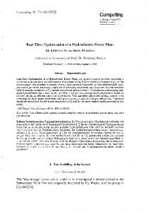
Table A.1: Key for Figure A-1

115

FLASH DETECTOR/LIGHT METER Vref

---

'

If3db = 2kHz I 6.8nF

1K INTO

PHOTO

IMICROPHONE| 1M

If3db = 87Hz 5.1

2.2uF

ADC1

1k

ADC2 52K

MIC

I

1luF

Ok

ISONAR DETECTOR I

ADC3 1

40kHz SONAR

1M

Figure A-i: Schematic diagram of the Pushpin Time of Flight Expansion Module

116

Bibliography [1] Pushpin Computing Web Page.

http://www.media.mit .edu/resenv/pushpin,

2004.

[2] Amorphous computing website. http://www.swiss.ai.mit.edu/projects/amorphous/, 2005.

[3] The network simulator - ns-2. http://www.isi.edu/nsnam/ns/, [4] Python Programming Language. http://www.python.org,

2005.

[5] SDCC - Small Device C Compiler. http://sdcc.sourceforge.net, [6] Silicon Laboratories. http://www.silabs.com, [7] Swarm. http://www.swarm.org/intro.html,

2005.

2005.

2005. 2005.

[8] Tinyos community forum. http://www.tinyos.net/,

2005.

[9] Harold Abelson, Don Allen, Daniel Coore, Chris Hanson, George Homsy, Jr. Thomas F. Knight, Radhika Nagpal, Erik Rauch, Gerald Jay Sussman, and Ron Weiss. Amorphous Computing . Communications of the ACM, May 2000. [10] Unknown Author.

Efficient Processing of Data for Locating Lightning Strikes.

Technical Brief KSC-12064/71, NASA Kennedy Space Flight Center, Unknown Year. [11] J. Bachrach. Position determination in sensor networks. to appear in Stojmenovic I (Ed), Mobile ad hoc networking, John Wiley and Sons, 2004. 117

RADAR: An In-Building RF-

[12] Paramvir Bahl and Venkata N. Padmanabhan.

based User Location and Tracking System. In Proceedings of IEEE INFOCOM, 2000.

[13] Sumit Basu, Steve Schwartz, and Alex Pentland.

Wearable Phased Arrays for

Sound Localization and Enhancement. In Fourth International Symposium on Wearable Computers (ISWC'00), page 103, 2000. [14] Pratik Biswas and Yinyu Ye. Semidefinite programming for ad hoc wireless sensor network localization. In Proceedings of the 2nd ACM international conference on wireless sensor networks and applications, pages 46 - 54, 2004. [15] Ingwer Borg.

Modern Multidimensional Scaling: Theory and Applications.

Springer, 1997.

[16] Michael Broxton, Joshua Lifton, and Joseph Paradiso. Localizing a Sensor Network via Collaborative Processing of Global Stimuli. In Proceedings of the European Conference on Wireless Sensor Networks (EWSN) 2005, 2005. [17] Nirupama Bulusu, Vladimir Bychkovskiy, Deborah Estrin, and John Heidemann. Scalable, ad hoc deployable rf-based localization. In Grace Hopper Celebration of Women in Computing Conference 2002, Vancouver, British Columbia, Canada., October 2002. [18] William Butera. Programming a Paintable Computer. PhD thesis, Massachusetts Institute

of Technology, 2002.

[19] Ramesh Govindan Chalermek Intanagonwiwat and Deborah Estrin. Making Sensor Networks Practical with Robots. In Sixth Annual International Conference on Mobile Computing and Networking, August 2000. [20] J.C. Chen, L. Yip, J. Elson, H. Wang, D. Maniezzo, R.E. Hudson, K. Yao, and D. Estrin.

Coherent Acoustic Array Processing and Localization on Wireless

Sensor Network. Proceedings of the IEEE, 98(8), August 2003. 118

[21] Crossbow Technologies. Intertial, Gyro, and Wireless Sensors from Crossbow. http://www.xbow.com,

2003.

[22] James W. Demmel. Applied Numerical Linear Algebra. SIAM, 1997. [23] Department of Integrative Medical Biology. Laboratory of Dexterous Manipula-

tion. http://www.humanneuro.physiol.umu.se/default.htm,

2004.

[24] S. Deutsch and A. Deutsch. Understanding the nervous system: an engineering perspective. IEEE Press, 1993. [25] M.A. Diftler and R.O. Ambrose. ROBONAUT, A Robotic Astronaut Assistant. ISAIRAS conference 2001, 2001.

[26] Lance Dohetry, Kristofer S. J. Pister, and Laurent El Ghaoui. Convex Position Estimation in Wireless Sensor Networks. In Proceedings of Infocom 2001, 2001. [27] L. Girod, V. Bychkobskiy, J. Elson, and D. Estrin.

Locating tiny sensors in

time and space: A case study. In Proceedings of the International Conference of

Computer Design (ICCD) 2002, 2002. [28] Lewis Girod and Deborah Estrin. Robust Range Estimated using Acoustic and Multi-modal Sensing. In Proceedings of the IEEE/RSJ

International Conference

on Intelligent Robots and Systems (IROS 2001), 2001. [29] Craig Gotsman and Yehuda Koren. Distributed graph layout for sensor networks. In Proceedings of the International Symposium on Graph Drawing, 2004. [30] Oliver Guenther, Tad Hogg, and Bernardo A. Huberman. Learning in multiagent control of smart matter. AAAI-97 Workshop on Multiagent Learning, 1997. [31] K. M. Hall. An r-dimensional quadratic placement algorithm. Science, 17:219 - 229, 1970. 119

Management

[32] T. He, C. Huang, B. Blum, J. Stankovic, and T. Abdelzaher. Range-Free Localization Schemes in Large Scale Sensor Networks. In Proceedings of the 9th annual international conference on Mobile computing and networking, pages 8195, 2003.

[33] Seth Hollar. COTS Dust. Master's thesis, University of California at Berkeley, 2000.

[34] Andrew Howard, Maja J Mataric, and Gaurav Sukhatme. Relaxation on a Mesh: a Formalism for Generalized Localization. In IEEE/RSJ International Conference on Intelligent Robots and Systems, Oct 2001. [35] A. Hu and S. D. Servetto. dfsk: Distributed frequency shift keying modulation in dense sensor networks. In Proceedings of the IEEE International Conference

on Communications (ICC), 2004. [36] Roland S. Johansson and Ake B. Valibo. Tactile sensory encoding in the glabrous skin of the human hand. Trends in Neuroscience, 6(1):27-32, 1983. [37] Yehuda Koren. On spectral graph drawing. In Proceedings of the 9th Interna-

tional Computing and Combinatorics Conference(COCOON'03), 2003. [38] Jack B. Kuipers.

Quaternions and Rotation Sequences. Princeton University

Press, 1999. [39] Anthony LaMarca, Waylon Brunnette, David Koizumi, Matthew Lease, Stefan B. Sigurdsson, Kevin Sikorski, Dieter Fox, and Gaetano Borriello. Making

Sensor Networks Practical with Robots. In Pervasive Computing First International Conference, pages 152-166, August 2002. [40] Koen Langendoen and Niels Reijers. Distributed localization in wireless sensor networks: a quantitative comparison.

The International Journal of Computer

and Telecommunication Networking, 43(4):499 - 518, November 2003. 120

[41] Joshua Lifton. Pushpin Computing: A Platform for Distributed Sensor Networks. Master's thesis, Massachusetts Institute of Technology, 2002. [42] Joshua Lifton, Deva Seetharam, Michael Broxton, and Joseph Paradiso. Pushpin Computing System Overview: a Platform for Distributed, Embedded, Ubiquitous Sensor Networks. In Proceedings of the International Conference on Pervasive Computing, August 2002. [43] Randolph L. Moses, Dushyanth Krishnamurthy, and Robert M. Patterson.

A

Self-Localization Method for Wireless Sensor Networks. EURASIP Journal on Applied Signal Processing, pages 348 - 358, 2003. [44] Radhika Nagpal. Organizing a Global Coordinate System from Local Information on an Amorphous Computer. A.I. Memo 1666, MIT Artificial Intelligence Laboratory,

1999.

[45] Radhika Nagpal, Howard Shrobe, and Jonathan Bachrach. Organizing a Global Coordinate System from Local Information on an Ad Hoc Sensor Network. In 2nd

International Workshop on Information Processing in Sensor Networks (IPSN '03), April 2003. [46] F. Paillet, D. Mercier, and T. Bernard. Second Generation Programmable Artificial Retina. In Proceedings of the IEEE ASIC/SOC Conference, pages 304-309, 1999.

[47] Thomas V. Papakostas, Julian Lima, and Mark Lowe. A large area force sensor for smart skin applications. In Proceedings of the IEEE Sensors 2002 Conference, 2002.

[48] Joseph Paradiso, Joshua Lifton, and Michael Broxton. Sensate Media - multimodal electronic skins as dense sensor networks. BT Technology Journal, 22(4), October 2004. [49] Neal Patwari and Alfred O. Hero III.

Using Proximity and Quantized RSS

for Sensor Localization in Wireless Networks. In Proceedings of the 2nd ACM 121

international conference on Wireless sensor networks and applications, pages 20 - 29, 2003.

[50] Neal Patwari and Alfred O. Hero III. Manifold learning algorithms for localization in wireless sensor networks. In Proceedings of the 2004 IEEE Int. Conf. on

Acoustics, Speech, and Signal Processing(ICASSP), May 2004. [51] Christina Peraki and Sergio D. Servetto. On the maximum stable throughput problem in random networks with directional antennas.

In Proceedings of the

ACM MOBIHOC 2003, 2003. [52] Arkady Pikovsky, Michael Rosenblum, and Jurgen Kurths. Synchronization: A universal concept in nonlinear sciences. Cambridge University Press, 2001. [53] Willian H. Press, Brian P. Flannery, Saul A. Teukolsky, and William T. Vetterling. Numerical Recipes in C: The Art of Scientific Computing. Cambridge University Press, 1988. [54] Nissanka B. Priyantha,

Hari Balakrishnan, Erik Demaine, and Seth Teller.

Anchor-Free Distributed Localization in Sensor Networks.

Tech Report 892,

MIT Laboratory for Computer Science, 2003. [55] Nissanka B. Priyantha, Anit Chakraborty, and Hari Balakrishnan. The cricket location-support system. In Mobile Computing and Networking, pages 32-43, 2000.

[56] Chip Redding, Floyd A. Smith, Greg Blank, and Charles Cruzan. Cots mems flow-measurement probes. Nanotech Briefs, 1(1):20, January 2004. [57] A. Savvides, W. Garber, S. Adlakha, R. Moses, and M. B. Srivastava. On the Error Characteristics of Multihop Node Localization in Ad-Hoc Sensor Networks. In Proceedings of the 2nd International Workshop on Information Processing in

Sensor Networks (IPSN'03), 2003. 122

[58] A. Savvides, H. Park, and M. Srivastava.

The Bits and Flops of the N-Hop

Multilateration Primitive for Node Localization Problems. In Proceedings of the

1st ACM international workshop on Wirelesssensor networks and applications, pages 112--121, 2002.

[59] Andreas Savvides, Chih-Chieh Han, and Mani B. Srivastava.

Dynamic fine-

grained localization in ad-hoc networks of sensors. In Mobile Computing and Networking, pages 166 - 179, 2001.

[60] M. Sergio, N.Manaresi, M. Tartagni, R. Guerrieri, and R.Canegallo. A textile based capacitive pressure sensor. In Proceedings of the IEEE Sensors 2002 Conference, 2002. [61] Yi Shang, Wheeler Ruml, Ying Zhang, and Markus P. J. Fromherz. Localization from Mere Connectivity. In Proceedings of the 4th A CM international symposium on mobile ad hoc networking and computing, pages 201 - 212, 2003. [62] Xiaohong Sheng and Yu-Hen Hu. Sensor deployment for source localization in wireless sensor network system. submitted to The First ACM Conference on Embedded Networked Sensor Systems, 2003. [63] Anthony Man-Cho So and Yinyu ye. Theory of Semidefinite Programming for Sensor Network Localization. To appear in SODA 2005, 2005. [64] Christopher Taylor, Ali Rahimi, Jonathan Bachrach, and Howard Shrobe. Simultaneous localization and tracking in an ad hoc sensor network. Submitted to IPSN 2005, 2005.

[65] Ben L. Titzer, Daniel K. Lee, and Jens Palsberg. Avrora: Scalable sensor network simulation with precise timing. In Proceedings of IPSN 2005, Fourth Interna-

tional Conferenceon Information Processingin Sensor Networks, 2005. [66] Andy Ward, Alan Jones, and Andy Hopper. A New Location Technique for the Active Office. IEEE Personal Communications, 4(5):42-47, October 1997. 123

[67] Brett Warneke, Matt Last, Brian Liebowitz, and Krisofer S. J. Pister. Smart dust:communicating with a cubic-millimeter computer.

Computer, 32:44 - 51,

2001.

[68] Rob Weiss. Cellular Computation and Communications using Engineered Genetic Regulatory Networks. PhD thesis, Massachusetts Institute of Technology, 2001.

[69] Kamin Whitehouse. The Design of Calamari: an Ad-hoc Localization System for Sensor Networks. Master's thesis, University of California at Berkeley, 2002. [70] Yong Xu, Yu-Chong Tai, Adam Huang, and Chih-Ming Ho. Ic-integrated flexible shear-stress sensor skin. Solid-State Sensor, Actuator and Microsystems Workshop, 2002.

124