Putting competing orders in their place near the Mott transition

Putting competing orders in their place near the Mott transition Leon Balents,1 Lorenz Bartosch,2, 3 Anton Burkov,1 Subir Sachdev,2 and Krishnendu Sengupta2 1 Department of Physics, University of California, Santa Barbara, CA 93106-4030 Department of Physics, Yale University, P.O. Box 208120, New Haven, CT 06520-8120 3 Institut f¨ ur Theoretische Physik, Universit¨ at Frankfurt, Postfach 111932, 60054 Frankfurt, Germany (Dated: August 13, 2004)

arXiv:cond-mat/0408329v4 [cond-mat.str-el] 7 Mar 2005

2

We describe the localization transition of superfluids on two-dimensional lattices into commensurate Mott insulators with average particle density p/q (p, q relatively prime integers) per lattice site. For bosons on the square lattice, we argue that the superfluid has at least q degenerate species of vortices which transform under a projective representation of the square lattice space group (a PSG). The formation of a single vortex condensate produces the Mott insulator, which is required by the PSG to have density wave order at wavelengths of q/n lattice sites (n integer) along the principle axes; such a second-order transition is forbidden in the Landau-Ginzburg-Wilson framework. We also discuss the superfluid-insulator transition in the direct boson representation, and find that an interpretation of the quantum criticality in terms of deconfined fractionalized bosons is only permitted at special values of q for which a permutative representation of the PSG exists. We argue (and demonstrate in detail in a companion paper: L. Balents et al., cond-mat/0409470) that our results apply essentially unchanged to electronic systems with short-range pairing, with the PSG determined by the particle density of Cooper pairs. We also describe the effect of static impurities in the superfluid: the impurities locally break the degeneracy between the q vortex species, and this induces density wave order near each vortex. We suggest that such a theory offers an appealing rationale for the local density of states modulations observed by Hoffman et al , Science 295, 466 (2002), in scanning tunnelling microscopy (STM) studies of the vortex lattice of Bi2 Sr2 CaCu2 O8+δ , and allows a unified description of the nucleation of density wave order in zero and finite magnetic fields. We note signatures of our theory that may be tested by future STM experiments.

I.

INTRODUCTION

One of the central debates in the study of cuprate superconductivity is on the nature of the electronic correlations in the ‘underdoped’ materials. At these low hole densities, the superconductivity is weak and appears only below a low critical temperature (Tc ), if at all. Nevertheless, there is no evidence of metallic behavior and an underlying Fermi surface of long-lived quasiparticles, as would be expected in a conventional BCS theory. This absence of Fermi liquid physics, and the many unexplained experimental observations, constitute key open puzzles of the field. In very general and most basic terms, the passage from optimal doping to the underdoped region may be characterized by an evolution from conducting (even superconducting) to insulating behavior. Indeed, most thinking on the cuprates is informed by their proximity to a Mott insulating state, in which interaction-induced carrier localization is the primary driving influence. Many recent attempts to describe the underdoped region have, by contrast, focused on the presence or absence of conventional orders (magnetism, stripe, superconductivity, etc.) as a means of characterization. This focus has practical merit, such orders being directly measured by existing experimental probes. Theoretically, however, the immense panoply of competing potential orders reduces the predictive power of this approach, which moreover obscures the basic conducting to insulating transition in action in these materials. In this paper, we describe a theoretical approach in which Mott localization is “back in

the driver’s seat”. Less colloquially, we characterize the behavior near to quantum critical points (QCPs) whose dual “order parameter” primarily describes the emergence of an insulating state from a superconducting one. Remarkably, a proper quantum mechanical treatment of this Mott transition leads naturally to the appearance of competing conventional orders. The manner in which this occurs is described in detail below. Among recent experiments, two classes are especially noteworthy for the issues to be discussed in our paper. Measurements of thermoelectric transport in a number of cuprates1 have uncovered a large Nernst response for a significant range of temperatures above Tc . This response is much larger than would be expected in a Fermi liquid description. However, a model of vortex fluctuations over a background of local superfluid order does appear to lead to a satisfactory description of the data1 . These experiments suggest a description of the underdoped state in terms of a fluctuating superconducting order parameter, Ψsc . Numerous such theories2 have been considered in the literature, under guises such as “preformed pairs” and “phase fluctuations”. Intriguing new evidence in support of such a “bosonic Cooper pair” approach has been presented in recent work by Kapitulnik and collaborators3. On the other hand, a somewhat different view of the underdoped state has emerged from a second class of experiments. Scanning tunnelling microscopy (STM) studies4–8 of Bi2 Sr2 CaCu2 O8+δ and Ca2−x Nax CuO2 Cl2 show periodic modulations in the electronic density of states, suggesting the appearance of a state with density wave order. Such density wave order can gap out portions of the Fermi surface, and so could be responsi-

2 ble for onset of a spin-gap observed in the underdoped regime. However, the strength of the density wave modulations is quite weak, and so it is implausible that they produce the large spin gap. The precise microscopic nature of the density wave modulations also remains unclear, and they could represent spatial variations in the local charge density, spin exchange energy, and pairing or hopping amplitudes. Using symmetry considerations alone, all of these modulations are equivalent, because they are associated with observables which are invariant under time-reversal and spin rotations. It is useful, therefore, to discuss a generic density wave order, and to represent it by density wave order parameters ρQ which determine the modulations in the ‘density’ by X δρ(r) = ρQ eiQ·r (1.1)

and the symmetry considerations above imply that F3 only contains terms which are products of terms already contained in F1 and F2 . In other words, only the energy densities of the two order parameters couple to each other, and neither order has an information on the local ‘orientation’ of the other order. The crucial coupling between the orders is actually in an oscillatory Berry phase term, but this leaves no residual contribution in the continuum limit implicit in the LGW analysis. To leading order in the order parameters, the terms in Eq. (1.4) are

where Q 6= 0 extends over some set of wavevectors. We will argue here that the apparent conflict between these two classes of experiments is neatly resolved by our approach. The strong vortex fluctuations suggest we examine a theory of superfluidity in the vicinity of a Mott transition. We will show that in a quantum theory of such a transition, which carefully accounts for the complex Berry phase terms, fluctuations of density wave order emerge naturally, and can become visible after pinning by impurities. Within the conventional Landau-Ginzburg-Wilson (LGW) theory9,10 , with the order parameters Ψsc and ρQ at hand, a natural next step is to couple them to each other. Here, one begins by writing down the most general effective free energy consistent with the underlying symmetries. A key point is that Ψsc and ρQ have non-trivial transformations under entirely distinct symmetries. The density wave order transforms under space group operations e.g. Ta , translation by the lattice vector a

The phase diagrams implied by the LGW functionals Eqs. (1.4) and (1.5) were determined by Liu and Fisher9 , and are summarized here in Fig 1. The transition between a state with only superconducting order (hΨsc i = 6 0, hρQ i = 0) and a state with only density wave order (hΨsc i = 0, hρQ i = 6 0) can follow one of 3 possible routes: (a) via a direct first order transition; (b) via an intermediate supersolid phase with both order parameters non-zero, which can be bounded by two second order transitions; and (c) via an intermediate “disordered” phase with both order parameters zero, which can also be bounded by two second order transitions. An important prediction of LGW theory is that there is generically no direct second order transition between the flanking states of Fig 1: such a situation requires fine-tuning of at least one additional parameter. While the predictions of LGW theory in Fig 1 are appropriate for classical phase transitions at nonzero temperatures, they develop a crucial shortcoming upon a naïve extension to quantum phase transitions at zero temperature. Importantly, the intermediate “disordered” phase in Fig 1 has no clear physical interpretation. At the level of symmetry, LGW theory informs us that this intermediate phase fully preserves electromagnetic gauge invariance and the space group symmetry of the lattice. Thinking quantum mechanically, this is not sufficient to specify the wavefunction of such a state. We could guess that this “disordered” state is a metallic Fermi liquid, which does preserve the needed symmetries. However, a Fermi liquid has a large density of states of low energy excitations associated with the Fermi surface, and these surely have to be accounted for near the quantum phase transitions to the other phases; clearly, such excitations are not included in the LGW framework. At a more sophisticated level, a variety of insulating states which preserve all symmetries of the Hamiltonian have been proposed in recent years12–14 , but these have a subtle ‘topological’ order which is not contained in the LGW framework. Such topologically ordered states have global (and possibly local) low energy excitations and these have to be properly accounted for near quantum critical

Q

Ta : ρQ → ρQ eiQ·a ; Ψsc → Ψsc ,

(1.2)

while Ψsc transforms under the electromagnetic gauge transformation, G, G : ρQ → ρQ ; Ψsc → Ψsc eiθ .

(1.3)

We could combine the two competing orders in a common ‘superspin’ order parameter (as in the ‘SO(5)’ theory11 ), but neither of the symmetry operations above rotate between the two orders, and so there is no a priori motivation to use such a language. The transformations in Eqs. (1.2) and (1.3) place important constraints on the LGW functional of Ψsc and ρQ , which can be written as F = F1 [Ψsc ] + F2 [ρQ ] + F3 [Ψsc , ρQ ] .

(1.4)

Here F1 is an arbitrary functional of Ψsc containing only terms which are invariant under Eq. (1.3), while F2 is a function of the ρQ invariant under space group operations like Eq. (1.2). These order parameters are coupled by F3 ,

F1 [Ψsc ] = r1 |Ψsc |2 + . . . X F2 [ρQ ] = r|Q| |ρQ |2 + . . . Q

F3 [Ψsc , ρQ ] =

X Q

v|Q| |Ψsc |2 |ρQ |2 + . . . .

(1.5)

3

Ψ sc ≠ 0

Ψ sc = 0

ρQ = 0

ρQ ≠ 0

Insulating solid

Superfluid

r1-r|Q|

(a) Ψ sc ≠ 0

Ψ sc ≠ 0

Ψ sc = 0

ρQ = 0

ρQ ≠ 0

ρQ ≠ 0

Superfluid

Supersolid

Insulating solid r1-r|Q|

(b) Ψ sc ≠ 0

ρQ = 0

Ψ sc = 0

ρQ = 0

"Disordered"

Ψ sc = 0

ρQ ≠ 0

Superfluid (= topologically Insulating solid ordered)

(c)

r1-r|Q|

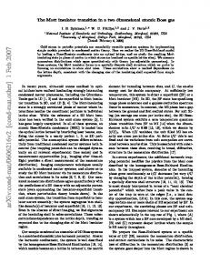
FIG. 1: LGW phase diagrams of the competition between the superconducting and density wave orders. The choice between the cases (a), (b), and (c) is made by the sign of v|Q| and by the values of the higher order couplings in (1.5). The thick line is a first order transition, and the thin lines are second order transitions. The “disordered” phase of LGW theory preserves all symmetries but is not the ‘topologically ordered’ phase which also preserves all symmetries: LGW theory does not predict the degeneracies of the latter state on topologically non-trivial spatial manifolds. It is believed there is no such “disordered” quantum state in the underlying quantum system at T = 0.

points15 ; again, such excitations are entirely absent in the LGW framework. Thus the purported existence of a truly featureless intermediate “disordered” state in Fig 1c suggests serious shortcomings of the LGW description of multiple order parameters in quantum systems13–16 . Conceptually, it is useful to emphasize that the LGW approach to the conducting–insulating transition is quite the reverse of the Mott picture. Indeed, the above symmetry considerations do not at all refer to transport, or to localization of the carriers. To address such properties, a conventional application of the LGW method would be to introduce the ρQ and Ψsc order parameters by a mean-field decoupling of a quantum model of bosons17 or fermions18 . These order parameters, once established, appear then as perturbations to the “quasiparticles” in the decoupled model. If ρQ becomes strong enough, the coincident potential barriers can localize the

carriers. Thus in the LGW approach the Mott transition eventually arises out of the competing order, not viceversa. In this paper, we will present an alternative approach to studying the interplay between the superfluid and density wave ordering in two spatial dimensions. Our analysis is based upon the recent work of Senthil et al.15 (and its precedents13,14,16 ), although we will present a different perspective. Also, the previous work15 was focused on systems at half-filling, while our presentation is applicable to lattice systems at arbitrary densities. One of the primary benefits of our approach is that the formalism naturally excludes the featureless ‘disordered’ states that invariably appear in the more familiar LGW framework. Our theory also makes it evident that the experimental observations of ‘phase’ fluctuations and pinned density wave order noted earlier are closely tied to each other, and, in principle, allows a compact, unified description of these experiments and also of the pinned density wave order around vortices in the superconductor19 . We will present our results here in the context of boson systems: specifically, in a general model of bosons hopping on a square lattice with short-range interactions. However, all the results of this paper apply essentially unchanged to electronic systems with short-range pairing. This is clearly the case for a toy model in which electrons experience a strong attractive interaction in the s-wave (or d-wave, though this is less obvious) channel, causing them to form tightly bound “molecular” Cooper pairs. Below the pair binding energy – i.e. the gap to unbound electron excitations – a description of the physics in terms of bosonic Cooper pairs clearly applies within such a model. Since we discuss universal physics near a bosonic superfluid to charge ordered transition, the theory here clearly describes such a transition from a short-range paired (also called the “strong pairing” regime/phase) superconductor to a density-wave ordered phase of any model, provided the electronic gap is maintained throughout the critical region. As we discuss below, a key parameter determining the character of the theories presented here is the number f , which for the lattice boson models is the average density of bosons per site of the square lattice in the Mott insulating state. Clearly, for electrons on the lattice with filling 1 − δ, i.e. hole density δ relative to half-filling, the density of bosonic Cooper pairs is f=

1−δ . 2

(1.6)

We note in passing that the density of carriers in the superfluid proximate to the Mott insulator is allowed to be different from that of the Mott insulator, as elaborated in Section II F. These features will be explicitly demonstrated in a companion paper20 , hereafter referred to as II. We argue in II that a convenient phenomenological model for capturing the spin S = 0 sector of electrons near a superfluidinsulator transition is the doped quantum dimer model

4 of the cuprate superconductors proposed by Fradkin and Kivelson21 . At zero hole concentration, the quantum dimer model22 generically has a Mott insulating ground state with valence bond solid (VBS) order16,23 (this order constitutes a particular realization of the generalized density wave order discussed above). Above some finite hole density, the dimer model has a superconducting ground state in which neutral observables preserve all lattice symmetries. (As we will discuss in II, the electronic pairing in this superconductor could have a d- or s(or other) wave character, depending upon microscopic details not contained in the dimer model). The evolution of the phase diagram between the insulating VBS state and the superconductor can occur via many possible sequences of transitions, all of which will be shown to be equivalent to those in the simpler boson models discussed in the present paper. A duality analysis of the doped dimer model presented in II directly gives the expected relation, Eq. (1.6). The paper II will also extend the dimer model to include fermionic S = 1/2 excitations: this theory will be shown to have a close connection to other24 U(1) or SU(2) gauge-theoretic “slave-particle” approaches to cuprate physics. Alternative formulations appropriate to long-range paired superconducting states (i.e. those with gapless nodal quasiparticle excitations) will also be discussed in II. Let us turn, then, to a model of bosons hopping on a square lattice, with short-range interactions,61 and at a density f per site of the square lattice. Our primary technical tool will be a dual description of this boson system using vortex degrees of freedom25–27 . Briefly, the world lines of the bosons in three-dimensional spacetime are reinterpreted as the trajectories of vortices in a dual, classical, three-dimensional ‘superconductor’ with a dual ‘magnetic’ field oriented along the ‘time’ direction. The dual superconducting order parameter, ψ, is the creation and annihilation operator for vortices in the original boson variables. The density of the vortices in ψ should equal the density of the bosons, and hence the dual ‘magnetic’ field acting on the ψ has a strength of f flux quanta per unit cell of the dual square lattice. It is valuable to characterize the phases in Fig 1 in terms of the dual field ψ. It is easy to determine the presence/absence of superfluid order (which is associated with the presence/absence of a condensate in Ψsc ). This has a dual relationship to the dual ‘superconducting’ order and is therefore linked to the absence/presence of a condensate in ψ: Superfluid : hψi = 0 Insulator : hψi = 6 0.

(1.7)

A condensate in ψ implies a proliferation of vortices in Ψsc , and hence the loss of superfluid order. Strictly speaking, the loss of superfluidity does not necessarily require the appearance of a condensate of elementary vortices. It is sufficient that at least a composite of n vortices condense, with hψ n i = 6 0, where n is a positive integer. The insulating states with n > 1 and hψi = 0

have topological order12 . For simplicity, we will not consider such insulating states here, although it is not difficult to extend our formalism to include such states and the associated multi-vortex condensates. The characterization of the density wave order in terms of the vortex field, ψ, is more subtle, and a key ingredient in our analysis. We have noted that the field ψ experiences a dual magnetic field of strength f flux quanta per unit cell. Consequently, just as is familiar from the Hofstadter problem of electrons moving in a crystal lattice in the presence of a magnetic field28,29 , the ψ Hamiltonian transforms under a projective representation of the space group30,31 or a PSG. A central defining property of a projective representation is that the operations Tx , Ty of translation by one lattice site along the x, y directions do not commute (as they do in any faithful representation of the space group), but instead obey Tx Ty = ωTy Tx ,

(1.8)

ω ≡ e2πif .

(1.9)

where

The PSG also contains elements corresponding to all other members of the square lattice space group. Among dual (rotation by angle π/2 about a site of the these are Rπ/2 dual lattice i.e. the sites of the lattice upon which the vortex field ψ resides) and Ixdual , Iydual (reflections about the x, y axes of the dual lattice); these obey32 group multiplication laws identical to those in the ordinary space group, e.g. dual −1 dual Ty = Rπ/2 Tx Rπ/2 dual dual Tx = Rπ/2 Ty Rπ/2 4 dual = 1. Rπ/2

(1.10)

All the elements of the PSG are obtained by taking arbitrary products of the elements already specified. A useful and explicit description of this projective representation is obtained by focusing on the low energy and long wavelength fluctuations of ψ at boson density f=

p q

(1.11)

where p and q are relatively prime integers. We assume that the average density in the Mott insulator has the precise commensurate value in Eq. (1.11). In most of the paper we will also assume that the superfluid has the density value in Eq. (1.11), but it is not difficult to extend our analysis to allow the density of the superfluid (or supersolid) to stray from commensurate values to arbitrary incommensurate values: this will be discussed in Section II F. As we will review in Section II, the spectrum of ψ fluctuations in the phase with hψi = 0 has q distinct minima in the magnetic Brillouin zone. We can use these minima to define q complex fields, ϕℓ , ℓ = 0, 1, . . . , q − 1

5 which control the low energy physics. These q vortex fields play a central role in all our analyses, as they allow us to efficiently characterize the presence or absence of superfluid and/or density wave order. In a convenient Landau gauge, the q vortex fields can be chosen to transform under Tx and Ty as Tx : ϕℓ → ϕℓ+1 Ty : ϕℓ → ϕℓ ω −ℓ .

(1.12)

Here, and henceforth, the arithmetic of all indices of the ϕℓ fields is carried out modulo q, e.g. ϕq ≡ ϕ0 . The action of all the PSG elements on the ϕℓ will be specified in Section II B; here we also note the important transfordual mation under Rπ/2 q−1 1 X dual Rπ/2 : ϕℓ → √ ϕm ω −mℓ , q m=0

(1.13)

which is a Fourier transform in the space of the q fields. It is instructive to verify that Eqs. (1.12) and (1.13) obey Eqs. (1.8) and (1.10). The existence of q degenerate species of vortices in the superfluid is crucial to all the considerations of this paper. At first sight, one might imagine that quantum tunnelling between the different vortex species should lift the degeneracy, and we should only focus on the lowest energy linear combination of vortices. However, while such quantum tunnelling may lead to a change in the preferred basis, it does not lift the q-fold degeneracy. The degeneracy is imposed by the structure of the PSG, in particular the relation Eq. (1.8), and the fact that the minimum dimension of a PSG representation is q. Using the transformations in Eqs. (1.12) and (1.13), we can now easily construct the required density wave order parameters ρQ as the most general bilinear, gaugeinvariant combinations of the ϕℓ with the appropriate transformation properties under the square lattice space group. The density wave order parameters appear only at the wavevectors Qmn = 2πf (m, n),

(1.14)

where m, n are integers, and take the form ρmn ≡ ρQmn = S (|Qmn |) ω mn/2

q−1 X

ϕ∗ℓ ϕℓ+n ω ℓm . (1.15)

ℓ=0

Here S(Q) is a general ‘form-factor’ which cannot be determined from symmetry considerations, and has a smooth Q dependence determined by microscopic details and the precise definition of the density operator. It is easy to verify that ρ∗mn = ρ−m,−n , and from Eqs. (1.12) and (1.13) that the space group operations act on ρmn just as expected for a density wave order parameter Tx : ρmn → ω −m ρmn Ty : ρmn → ω −n ρmn

dual : ρmn → ρ−n,m . Rπ/2

(1.16)

So by studying the bilinear combinations in Eq. (1.15), we can easily characterize the density wave order in terms of the ϕℓ . It is worth reiterating here that the ρmn order parameters in Eq. (1.15) are generic density wave operators, and could, in principle, be adapted to obtain the actual density of either the bosons or the vortices. Indeed, as we noted above Eq. (1.1), we can obtain information on arbitrary observables invariant under spin rotations and time reversal, including the local density of states. The different specific observables will differ only in their values of the form factor S(Q), which we do not specify in the present paper. Note also that because the dual Rπ/2 rotation is about a dual lattice site, the last relation in Eq. (1.16) implies that the Fourier components ρQ are defined by taking the origin of the spatial co-ordinates on a dual lattice site. Upon performing the inverse Fourier transform from the ρmn to real space (as in Eq. (2.26) below) the resulting density gives a measure (up to a factor of the unknown S(Q)) of the vortex density on the dual lattice sites, and of the boson density on the direct lattice sites.62 For completeness, we note that the characterizations in Eq. (1.7) of the superfluid order in terms of the vortex fields has an obvious expression in terms of the ϕℓ : Superfluid : hϕℓ i = 0 for every ℓ Insulator : hϕℓ i = 6 0 for at least one ℓ. (1.17) The key relations in Eqs. (1.15) and (1.17) allow us to obtain an essentially complete characterization of all the phases of the boson model of interest here: this is a major reason for expressing the theory in terms of the vortex fields ϕℓ . Furthermore, the symmetry relations in Eqs. (1.12) and (1.13) impose strong constraints on the effective theory for the ϕℓ fields whose consequences we will explore in Section II C. Indeed, even before embarking upon a study of this effective theory, we can already see that our present theory overcomes one of the key shortcomings of the LGW approach. We note from Eq. (1.17) that the non-superfluid phase has a condensate of one or more of the ϕℓ . Inserting these condensates into Eq. (1.15) we observe that hρmn i = 6 0 for at least one nonzero Qmn i.e. the non-superfluid insulator has density wave order. Consequently the intermediate “disordered” phase in Fig 1c has been automatically excluded from the present theory. Instead, if the ϕℓ condensate appears in a second-order transition (something allowed by the general structure of the theory), we have the possibility of a generic second-order transition from a superfluid phase to an insulator with density wave order, a situation which was forbidden by the LGW theory.63 We summarize the possible phase diagrams of the ϕℓ theory in Fig 2. In addition to characterizing modulations in the “density” in terms of the ρmn , the ϕℓ fields can also determine modulations in the local vorticity. This is a measure of circulating boson currents around plaquettes of the direct lattice33 , and has zero average in all phases because time-reversal invariance is preserved. However, in the

6

ϕl = 0

ϕl = 0

ρ mn = 0

ρ mn = 0 Insulating solid

Superfluid

r1-r|Q|

(a) ϕl = 0

ϕl = 0

ϕl = 0

ρ mn = 0

ρ mn = 0

ρ mn = 0

Superfluid

Supersolid

Insulating solid r1-r|Q|

(b) ϕl = 0

ϕl = 0

ρ mn = 0

ρ mn = 0

Superfluid

Insulating solid

(c)

r1-r|Q|

FIG. 2: Possible phase diagrams in the vortex theory of the interplay of superfluid and density wave order. Conventions are as in Fig 1. Notice that the objectionable “disordered” phase of the LGW theory has disappeared, and is replaced by a direct second order transition. Also, the first order transition in (a) is “fluctuation induced”, i.e. unlike the LGW theory of Fig 1, the mean field vortex theory only predicts a second order transition, but fluctuations could induce a weak first order transition.

presence of an applied magnetic field, this constraint no longer applies. The magnetic field, of course, induces a net circulation of boson current, and the total number of vortices (or anti-vortices) is non-zero. However, using a reasoning similar to that applied above to the density, the PSG of the vortices implies there are also modulations in the vorticity at the Qmn wavevectors. We can define a corresponding set of Vmn which are Fourier components of the vorticity at these wavevectors. Details of this analysis, and explicit expressions for the Vmn appear in Appendix A. An explicit derivation of the above vortex theory of the Mott transition of the superfluid appear in Section II where we consider a model of bosons on the square lattice. Here we derive an effective action for the q vortex species in Eqs. (2.19) and (2.21) which is invariant under the PSG, and which controls the phases and phase diagrams outlined above. A complementary perspective is presented in Section III where we formulate the physics using the direct

boson representation. In particular, following Senthil et al.15 , we explore the possibility that the LGW forbidden superfluid-insulator transitions discussed above are associated with the boson fractionalization. The structure of the theory naturally suggests a fractionalization of each boson into q components, each with boson number 1/q. However, the PSG places strong restrictions on the fractionalized boson theory. On the rectangular lattice, such a theory is consistent for all q but only for certain insulating phases obtained for restricted parameter values. On dual the square lattice, with the additional Rπ/2 element of the PSG, a fractionalized boson theory is permitted only for a limited set of q values. Specifically, it is required that the ϕℓ vortex fields transform under a permutative representation of the PSG. We define a permutative representation as one in which all group elements can be written as ΛP , where Λ is a unitary diagonal matrix (i.e. a matrix whose only non-zero elements are complex numbers of unit magnitude on the diagonal), and P is a permutation matrix. For the representation defined in Eqs. (1.12) and (1.13), Tx and Ty are of this form, while dual Rπ/2 is not. When a permutative representation exists, it is possible to globally unitarily transform the ϕℓ fields to a new basis of ζℓ fields, which realize the permutative representation. For some range of parameters – values of the quantum tunnelling terms between the vortex flavors – one can see that the PSG is expected to be elevated at the critical point to include an emergent U (1)q (modulo the global U (1) gauge invariance) symmetry of independent rotations of the ζℓ fields. This emergent symmetry is the hallmark of fractionalization, and corresponds to emergence of conserved U (1) gauge fluxes in the direct representation. Such an emergent symmetry is clearly not generic, and this turns out to place quite a restrictive condition on the existence of a fractionalized 1/q boson representation, as we discuss in detail in Section III, and in a number of appendices. Section IV applies our theory to the STM observations of local density of states modulations in zero and nonzero magnetic field. A virtue of our approach is that it naturally connects density wave order with vorticity and allows a unified description of the experiments in zero and non-zero magnetic field. As we will discuss, there are several intriguing consequences of our approach, and we will analyze prospects for observing these in future STM experiments in Sections IV and V. We briefly mention other recent works which have addressed related issues. Zaanen et al.34 have examined the superfluid to insulator transition from a complementary perspective: they focus on the dislocation defects of a particular insulating solid in the continuum, in contrast to our focus here on the vortex defects of the superfluid. We do consider the ‘melting’ of defects in the solid in Section III C, but the underlying lattice plays a crucial role in our considerations. In a work which appeared while our analysis was substantially complete, Teˇsanović35 has applied the boson-vortex duality to Cooper pairs and considered the properties of vortices in a dual ‘magnetic’

7 field.

II.

DUAL VORTEX THEORY OF BOSONS ON THE SQUARE LATTICE

We consider an ordinary single-species boson model on the square lattice. The bosons are represented by rotor operators φî and conjugate number operators n ˆ i where i runs over the sites of the direct square lattice. These operators obey the commutation relation [φî , n ˆ j ] = iδij .

(2.1)

A simple boson Hamiltonian in the class of interest has the structure X X V (ˆ ni ) cos ∆α φî − 2πgiα + H = −t iα

+

X

as Feynman integral over states at a large number of intermediate time slices, separated by the interval ∆τ . The intermediate states use a basis of n ˆ i and φî at alternate times. The hopping term in H acts between φî eigenstates, and we evaluate its matrix elements by using the Villain representation exp t∆τ cos ∆α φî − 2πgiα X J2 exp − iα + iJiα ∆α φî − 2πiJiα giα . (2.4) → 2t∆τ {Jiα }

We have dropped an unimportant overall normalization constant, and will do so below without comment. The Jiα are integer variables residing on the links of the direct lattice, representing the current of the bosons. After integrating over the φi on all sites and at all intermediate times, the partition function becomes

i

Λij n în ˆj + . . .

(2.2)

i6=j

where the interaction V (ˆ n) has the on-site terms V (ˆ n) = −¯ µn ˆ + Un ˆ (ˆ n − 1)/2. The Λij are repulsive off-site interactions, and can also include the long-range Coulomb interaction. We will focus on the case of short-range Λij , and note the minor modifications necessary for the longrange case. The general structure of our theory also permits a variety of exchange and ring-exchange terms, such as those in the studies of Sandvik et al.36 . These off-site or ring exchange couplings are essential for our analysis, as they are needed to stabilize insulating phases of the bosons away from integer filling. Nevertheless, many aspects of our results are independent upon the particular form of these couplings; their specific form will only influence the numerical values of the non-linear couplings that appear in our phenomenological actions (such as those in Eq. (2.21)). The index α extends over the spatial directions x, y, while we will use indices µ, ν, λ to extend over all three spacetime directions x, y, τ . The symbol ∆α is a discrete lattice derivative along the α direction: ∆α φî = φî+α − φˆ (and similarly for ∆µ ). We have also included a static external magnetic field represented by the vector potential giα for convenience. This is a uniform field which obeys ǫµνλ ∆ν giλ = hδµτ

(2.3)

where h is the strength of the physical magnetic field (which should be distinguished from the dual “magnetic” flux f discussed in Section I).

Z =

X

{Jiµ }

exp −

− ∆τ

X

1 X (Jiµ − Hδµτ )2 2e2 i !

Λij Jiτ Jjτ − 2πigiµ Jiµ

i6=j

×

Y

δ (∆µ Jiµ )

(2.5)

i

where Jiµ ≡ (ni , Jix , Jiy ) is the integer-valued boson current in spacetime, i now extends over the sites of the cubic lattice, and we have chosen ∆τ so that e2 = t∆τ = 1/U ∆τ , and H = µ ¯/U + 1/2. We now solve the constraint in Eq. (2.5) by writing Jiµ = ǫµνλ ∆ν Aaλ

(2.6)

where a labels sites on the dual lattice, and Aaλ is an integer-valued gauge field on the links of the dual lattice. We promote Aaµ from an integer-valued field to a real field by the Poisson summation method, while “softening” the integer constraint with a fugacity yv . It is convenient to make the gauge invariance of the dual theory explicit by introducing an angular field ϑa on the sites of the dual lattice, and mapping 2πAaµ → 2πAaµ − ∆µ ϑa . The operator eiϑa is then the creation operator for a vortex in the boson phase variable φi . These transformations yield the dual partition function Zd =

YZ a

dAaµ

Z

dϑa exp

1 X 2 (ǫµνλ ∆ν Aaλ − Hδµτ ) 2e2 2 X + yv cos (∆µ ϑa − 2πAaµ ) −

A.

Dual lattice representation

aµ

We proceed with a standard duality mapping, following the methods of Refs. 25–27 and the notational conventions of Ref. 37. We represent the partition function

− ih

X a

!

(∆τ ϑa − 2πAaτ ) .

(2.7)

8 We have not explicitly displayed the Λij term above, and assumed it has been absorbed into a renormalized value of e2 .64 This is the theory of a dual vortex boson represented by the angular rotor variable ϑa , coupled to a dual gauge field Aaµ . The Berry phase term proportional to h is precisely the constraint that the rotor number variable (canonically conjugate to ϑa ) takes values which are integers plus h (see Ref. 27): so there is a background density of vortices of h per site which is induced by the magnetic field acting on the direct bosons. The remainder of Section II will consider only the case h = 0; the analog of the h 6= 0 case will appear later in the dimer model analyses of II. We obtain the dual theory in its final form on the cubic lattice by replacing the field eiϑa by a “soft-spin” dual vortex field ψa , which yields Z YZ Zd = dAaµ dψa exp a

1 X 2 (ǫµνλ ∆ν Aaλ − Hδµτ ) 2e2 2 yv X ∗ ψa+µ e2πiAaµ ψa + c.c. + 2 aµ ! i Xh u 2 4 s|ψa | + |ψa | . (2.8) − 2 a

−

The last line in Eq. (2.8) is the effective potential for the complex vortex field ψa . Increasing the parameter s scans the system from the insulating solid at s ≪ 0 to the superfluid at s ≫ 0 ı.e. the system moves from right to left in the phase diagrams of Fig 2. B.

Symmetries

We will now present a careful analysis of the symmetries of Eq. (2.8), with the aim of deducing general constraints that must be obeyed by the low energy theory near the superfluid-to-insulator transition. We begin in the superfluid regime with s large, so that hψa i = 0. The direct boson density is the τ component of the dual ‘magnetic’ flux ǫµνλ ∆ν Aλ , and for s large in the action in Eq. (2.8) it is clear that the saddle point of the Aµ fluctuations occurs at Aaµ = Aaµ with ǫµνλ ∆ν Aaλ = Hδµτ . We want this boson density to be the value f in Eq. (1.11), and so we should choose H = f . We now wish to examine the structure of ψa fluctuations about this saddle point. Let us choose the Landau gauge with Aaτ = Aax = 0 and Aay = f ax ;

(2.9)

here ax is the x co-ordinate of the dual lattice a. We now need to determine the ψa spectrum in a background Aaµ field. dual The basic symmetry operations are Tx , Ty , and Rπ/2 , introduced in Section I. The action of these operators on

ψa ≡ ψ(ax , ay ) required to keep the Hamiltonian invariant is Ty : ψ(ax , ay ) → ψ(ax , ay − 1) Tx : ψ(ax , ay ) → ψ(ax − 1, ay )ω ay

dual : ψ(ax , ay ) → ψ(ay , −ax )ω ax ay Rπ/2

(2.10)

Notice that Eqs. (1.8) and (1.10) are obeyed by the above. It is also useful to collect the representation of Eq. (2.10) in momentum space. Implying that all momenta are reduced back to the extended Brillouin zone with momenta −π < kx , ky < π we find Ty : ψ(kx , ky ) → ψ(kx , ky )e−iky

Tx : ψ(kx , ky ) → ψ(kx , ky − 2πf )e−ikx

dual Rπ/2 : ψ(kx , ky ) →

(2.11)

q−1 X

1 ψ(ky + 2πnf, −kx − 2πmf )ω −mn q m,n=0 The most important ψa fluctuations will be at momenta at which the spectrum has minima. It is not difficult to show from the above symmetry relations that any such minimum is at least q-fold degenerate: Let |Λi be a state at a minimum of the spectrum. Because, the operator Ty commutes with the Hamiltonian, this state can always be chosen to be an eigenstate of Ty , with eigen∗ value e−iky . Now the above relations imply immediately that Tx |Λi is also an eigenstate of the Hamiltonian with ∗ Ty eigenvalue e−iky ω −1 . Also, because the Ty eigenvalue is distinct from that of |Λi, this state is an orthogonal eigenstate of the Hamiltonian. By repeated application of this argument, we obtain q orthogonal eigenstates of the ∗ Hamiltonian whose Ty eigenvalues are e−iky times integer powers of ω −1 . Because we are working with the gauge of Eq. (2.9), our Hamiltonian couples momenta (kx , ky ) to momenta (kx ± 2πf, ky ). It is therefore advantageous to look at the spectrum in the reduced Brillouin zone with −π/q < kx < π/q and −π < ky < π. For the nearestneighbor model under consideration here, the minima of the spectrum are then at the q wavevectors (0, 2πℓp/q) with ℓ = 0, . . . q − 1. Let us label the eigenmodes at these wavevectors ϕℓ . We therefore have to write down the field theory in terms of these q complex fields ϕℓ . It is useful, especially when analyzing the influence of dual Rπ/2 , to make the above symmetry considerations explicit. In the extended Brillouin zone, for the nearestneighbor model under consideration here, let us label the q 2 states at the wavevectors (2πmp/q, 2πnp/q) by |m, ni. Then one of the minima of the spectrum corresponds to the state |ϕ0 i =

q−1 X

m=0

cm |m, 0i

(2.12)

where the cm are some complex numbers. Then, by operation of Tx on |ϕ0 i we obtain the q degenerate eigenstates

9 as |ϕℓ i =

q−1 X

m=0

cm ω −ℓm |m, ℓi

(2.13)

dual Now let us consider the action of Rπ/2 on the states in Eq. (2.13). Using Eq. (2.11), and after some simple changes of variables we obtain

dual |ϕℓ i = Rπ/2

1 q

q−1 X

′ ′

m,m′ ,ℓ′ =0

′

′

cm ω −(m ℓ +ℓℓ −mm ) |m′ , ℓ′ i

(2.14) dual Now, because Rπ/2 commutes with H, the right-handside of Eq. (2.14) must be a linear combination of the |ϕℓ i states in Eq. (2.13). The matrix elements of the rota′ dual tion operator are then given by hϕℓ′ |Rπ/2 |ϕℓ i = c ω −ℓℓ , P ′ where c = q1 c∗m′ cm ω mm is independent of ℓ and ℓ′ . For the nearest-neighbor model under consideration here, it can be easily checked that the cm ’s are invariant under √ a Fourier transform such that c = 1/ q. Hence we find q−1 1 X −ℓℓ′ dual ω |ϕℓ′ i. Rπ/2 |ϕℓ i = √ q ′

(2.15)

ℓ =0

Our discussion above has now established that the low energy vortex fields must have an action invariant under the transformations in Eqs. (1.12) and (1.13). In a similar manner we can also determine the transformations associated with the remaining elements of the square lattice space group. These involve the operations Ixdual and Iydual which are reflections about the x and y axes of the dual lattice. Under these operations we find Ixdual Iydual

: ϕℓ → : ϕℓ →

ϕ∗ℓ ϕ∗−ℓ

.

(2.16)

Finally it is interesting to consider the point inversion dual 2 operator Ipdual ≡ (Rπ/2 ) , with Ipdual : ϕℓ → ϕ−ℓ .

(2.17)

As in the ordinary space group we have Ipdual = Ixdual Iydual = Iydual Ixdual .

(2.18)

will be represented by the continuum non-compact U(1) gauge field aAµ /(2π), where a is the lattice spacing. First, we consider quadratic order terms about the saddle point of Eq. (2.8). The most general action has the familiar terms of scalar electrodynamics S0 =

Z

2

d rdτ

q−1 X ℓ=0

|(∂µ − iAµ )ϕℓ |2 + s|ϕℓ |2

1 2 + (ǫµνλ ∂ν Aλ ) . 2e2

(2.19)

We have rescaled the coupling e here by a factor of 2π from Eq. (2.8). Next, we consider terms which are quartic in the ϕℓ , but which contain no spatial or temporal derivatives. These will be contained in the action S1 . We discuss two approaches to obtaining the most general quartic invariants. The first is the most physically transparent, but turns out to be eventually inconvenient for explicit computations. In this approach we use density operators defined in Eq. (1.15), and their simple transformation properties in Eq. (1.16), to build up quartic invariants. In particular, the quartic invariants are only quadratic in the ρmn , and we need only the most general quadratic term invariant under Eq. (1.16). This has the form S1 =

Z

2

d rdτ

q/2 n X X

n=0 m=0

λnm |ρnm |2 + |ρn,−m |2

2

2

+|ρmn | + |ρm,−n |

!

(2.20)

However, not all the invariants above are independent, and there are often linear relations between them - this reduces the number of independent coupling constants λnm . Determining the linear relations between the couplings turns out to be inconvenient, and we found it easier to proceed by the second method described below. In the second approach, we first impose only the constraints imposed by the translation operations Tx , Ty . By inspection, it is easy to see that the most general quartic term invariant under these operations has the structure Z X 1 S1 = d2 rdτ γmn ϕ∗ℓ ϕ∗ℓ+m ϕℓ+n ϕℓ+m−n . (2.21) 4 ℓmn

C.

Continuum field theories

We have established that fluctuations of the vortex fields about the saddle point of Eq. (2.8) in Eq. (2.9) transform under a projective representation of the square lattice space group which is defined by Eqs. (1.12), (1.13), and (2.16). In this section we will write down the most general continuum theory of the ϕℓ fields which is invariant under these projective transformations. The action should include fluctuations in Aaµ about Aaµ – this

Here the integers ℓ, m, n, . . . range implicitly from 0 to q − 1 and all additions over these integers are taken modulo q. Imposing in addition the reflection operations in Eq. (2.16), and accounting for the internal symmetries in Eq. (2.21), it is easy to show that the couplings γmn can always be taken to be real and to obey the relations γmn = γ−m,−n γmn = γm,m−n γmn = γm−2n,−n .

(2.22)

10 We have so far not yet imposed the constraints implied dual by the lattice rotation Rπ/2 . Consequently, Eqs. (2.21) and (2.22) define the most general quartic terms for a system with rectangular symmetry, which may be appropriate in some physical situations. By explicit solution of the constraints defined by Eq. (2.22), we found that the quartic terms are determined by Nrect independent real coupling constants, where Nrect =

(n + 1)(n + 2) for q = 2n, 2n + 1, 2

(2.23)

with n a positive integer. Note that the number of couplings grows quite rapidly with increasing q: Nrect ∼ q 2 /8. dual Finally, let us consider the consequences of the Rπ/2 symmetry. By applying Eq. (1.13) to Eq. (2.21) we find that S1 remains invariant provided the γmn obey the relations 1X ¯ n)+¯ n(m−n)] γm¯ γmn ω −[n(m−¯ (2.24) ¯n = q mn Naïvely, there are q 2 relations implied by Eq. (2.24), but they are not all independent of each other. By explicitly solving the relations in Eq. (2.24) for a range of q values we found that the number of independent quartic coupling constants for a system with full square lattice symmetry is (n + 1)2 for q = 4n, 4n + 1 Nsquare = (n + 1)(n + 2) for q = 4n + 2, 4n + 3 (2.25) with n a positive integer. The additional restrictions of square relative to rectangular symmetry reduce the number of independent coupling constants by roughly half at large q: Nsquare ∼ q 2 /16. D.

Mean field theory

This section will examine the mean-field phase diagrams of the general theory S0 + S1 proposed in Section II C. From the discussion in Section I, it is clear that such a procedure can yield a direct second order transition from a superfluid state (with hϕℓ i = 0) to an insulating state with density wave order (with hϕℓ i = 6 0). We are interested in determining the possible configurations of values of the ϕℓ and the associated patterns of density wave order for a range of q values (in this subsection, we will simply write hϕℓ i as ϕℓ because there is no distinction between the two quantities in mean field theory). After determining the ϕℓ , we determined the ρmn by Eq. (1.15) (using a Lorentzian for the form factor S(Q) = 1/(1 + Q2 )), and then computed the density wave order using δρ(r) =

q−1 X

m,n=−q

ρmn e2πif (mrx +nry )

(2.26)

We evaluated Eq. (2.26) at r values corresponding to the sites, bonds, and plaquettes of the direct lattice, and plotted the results in the square lattice figures that appear below. In the formalism of Section II, r values with integer co-ordinates correspond to the sites of the dual lattice, and hence to plaquettes of the direct lattice. The value of δρ(r) on such plaquette co-ordinates can be considered a measure of the ring-exchange amplitude of bosons around the plaquette. By a similar reasoning, r values with half-odd-integer co-ordinates represent sites of the direct lattice, and the values of δρ(r) on such sites measure the boson density on these sites. Finally, r values with rx integer and ry half-odd-integer correspond to horizontal links of the square lattice (and vice versa for vertical links), and the values of δρ(r) on the links is a measure of the mean boson kinetic energy; if the bosons represent a spin system, this is a measure of the spin exchange energy. Our results appear for a range of q values in the following subsections.

1.

q=2

After imposing the symmetry relations in Eqs. (2.22) and (2.24), R the quartic potential in Eq. (2.21) (defined by S1 = d2 rdτ L4 ) is L4 =

2 γ01 γ00 |ϕ0 |2 + |ϕ1 |2 + (ϕ0 ϕ∗1 − ϕ∗0 ϕ1 )2 (. 2.27) 4 4

We now make the change of variables ζ0 + ζ1 √ 2 ζ0 − ζ1 = −i √ . 2

ϕ0 = ϕ1

(2.28)

As we will discuss in detail in Section III A, the new variables have the advantage of realizing a permutative representation of the PSG, i.e. all representation matrices of the PSG have only one non-zero unimodular element in every row and column. From Eqs. (1.12), (1.13), and (2.28) it is easy to deduce that in the ζℓ variables, 0 1 0 −i ; Ty = Tx = 1 0 i 0 0 e−iπ/4 dual . (2.29) Rπ/2 = eiπ/4 0 The action in Eq. (2.27) reduces to L4 =

2 γ01 2 γ00 |ζ0 |2 + |ζ1 |2 − |ζ0 |2 − |ζ1 |2 . (2.30) 4 4

The result in Eq. (2.30) is identical to that found in earlier studies13,14 of the q = 2 case. Minimizing the action implied by Eq. (2.30), it is evident that for γ01 < 0 there is a one parameter family of

11

A C B or A

0

FIG. 4: As in Fig 3 but for q = 3

gauge-invariant solutions in which the relative phase of ζ0 and ζ1 remains undetermined. Computing the values of δρ(r) establishes that this phase is physically significant, because it leads to distinguishable density wave modulations. This indicates that the phase will be determined by higher order terms in the effective potential. As shown in earlier work13 , one needs to go to a term which is eighth order in the ϕℓ before the value of arg(ζ0 /ζ1 ) is pinned at specific values. In the present formalism, the required eighth order term is ρ20,1 ρ21,0 , which is invariant under all the transformations in Eq. (1.16); this contains a term ∼ (ζ0 ζ1∗ )4 + c.c. Our specific results from the mean field theory for q = 2 are summarized in Fig 3. The state (A) has an ordinary charge density wave (CDW) at wavevector (π, π). The other two states are VBS states in which all the sites of the direct lattice remain equivalent, and the VBS order appears in the (B) columnar dimer or (C) plaquette pattern. The saddle point values of the fields associated with these states are: (A) : ζ0 6= 0 , ζ1 = 0 or ζ0 = 0 , ζ1 6= 0.

(C) : ζ0 =

6= 0,

2.

q=3

Now there are 3 ϕℓ fields, and the quartic potential in Eq. (2.27) is replaced by 2 γ00 |ϕ0 |2 + |ϕ1 |2 + |ϕ2 |2 4 γ01 ∗ ∗ 2 ϕ0 ϕ1 ϕ2 + ϕ∗1 ϕ∗2 ϕ20 + ϕ∗2 ϕ∗0 ϕ21 + c.c. + 2 . − 2|ϕ0 |2 |ϕ1 |2 − 2|ϕ1 |2 |ϕ2 |2 − 2|ϕ2 |2 |ϕ0 |2 (2.32)

L4 =

We show in Appendix E that there is now no transformation of the ϕℓ variables which realize a permutative representation of the PSG, and in which Eq. (2.32) may take a more transparent form. The results of the minimization of S0 + S1 for the insulating phases are shown in Fig 4. The states have stripe order, one along the diagonals, and the other along the principle axes of the square lattice. Both states are 6-fold degenerate, and the characteristic saddle point values of the fields are (A) : ϕ0 6= 0 , ϕ1 = ϕ2 = 0 or

ei4nπ/3 ϕ2 = ei2nπ/3 ϕ1 = ϕ0 = 6 0 (B) : ϕ0 = ϕ1 = e±2iπ/3 ϕ2 and permutations. (2.33) 3.

q=4

For q = 4, there are 4 independent quartic invariants in Eq. (2.21), and they can be combined into the following forms. 2 I1 = ρ20,0 = |ϕ0 |2 + |ϕ1 |2 + |ϕ2 |2 + |ϕ3 |2 2

I2 = ρ22,2 = (ϕ∗0 ϕ2 + ϕ∗2 ϕ0 − ϕ∗1 ϕ3 − ϕ∗3 ϕ1 )

inπ/2

ζ1 6= 0. i(n+1/2)π/2 e ζ1

γ01

0

γ01

FIG. 3: Mean field phase diagram of S0 + S1 defined in Eqs. (2.19) and (2.21). The couplings obey Eqs. (2.22) and (2.24). We assumed s = −1 to obtain an insulating state, and γ00 = 1. Plotted are the values of δρ(r), defined as in Eq. (2.26), on the sites, links and plaquettes of the direct lattice: the lines represent links of the direct lattice. As discussed in the text, these values represent the boson density, kinetic energy, and ring-exchange amplitudes respectively. The saddle point values of the fields in the states are shown in Eq. (2.31). The choice between the states B and C is made by a eighth order term in the action.

(B) : ζ0 = e

B

(2.31)

where n is any integer. At quartic order, the states B and C are degenerate with all states with ζ0 = eiθ ϕ1 , with θ arbitrary; the value of θ is selected only by the eighth order term.

I3 = |ϕ0 |2 |ϕ1 |2 + |ϕ1 |2 |ϕ2 |2 + |ϕ2 |2 |ϕ3 |2 + |ϕ3 |2 |ϕ0 |2 −ϕ∗0 ϕ∗1 ϕ2 ϕ3 − ϕ∗1 ϕ∗2 ϕ3 ϕ0 − ϕ∗2 ϕ∗3 ϕ0 ϕ1 − ϕ∗3 ϕ∗0 ϕ1 ϕ2 I4 = ϕ∗0 ϕ∗2 ϕ21 + ϕ23 + c.c. + ϕ∗1 ϕ∗3 ϕ20 + ϕ22 + c.c. − 4|ϕ0 |2 |ϕ2 |2 − 4|ϕ1 |2 |ϕ3 |2

(2.34)

Now as for q = 2, the invariants for q = 4 do simplify by redefinitions of the fields analogous to Eq. (2.28), which

12 realize a permutative representation of the PSG. We define ϕ0 = ϕ2 = ϕ1 = ϕ3 =

√ (ζ0 + ζ1 )/ 2 √ (ζ0 − ζ1 )/ 2 √ (ζ3 + ζ2 )/ 2 √ (ζ3 − ζ2 )/ 2.

v2 2

or

(2.35)

A: λ>0

B: λ 0. Due to fluctuations, the actual location of the critical point s = sc at which vortex condensation occurs is reduced to sc < 0. Thus one may expect that locally, for sc < ∼ s < 0, the ζℓ fields may develop some non-zero magnitude. This occurs because P of a balance between the negative quadratic term −|s| ℓ |ζℓ |2 and the quartic terms in L4 . From the form of the negative quadratic term, this balance clearly favors states with

pP 2 a non-zero generalized “radius” ℓ |ζℓ | in ζℓ space. The preferred directions in this 2q-dimensional (due to real and imaginary parts of each ζℓ ) space, however, are determined by the terms in L4 . To obtain a phase-only description, one needs that the dominant terms in L4 favor states with |ζℓ | = ϕ. This requirement places strong constraints on the form of one must have that, for fixed P L4 . 2 In particular, 2 |ζ | = qϕ , the minima of L4 satisfy |ζℓ | = ϕ for ℓ ℓ all ℓ. Explicit examples with rotational invariance can be seen for q = 2, 4 from Sec. II D 1,II D 3. For q = 2, this is true if γ01 < 0. For q = 4 this is true in region E when λ = 0. Thus if λ is irrelevant in region E at the QCP, the requirement is satisfied. On the other hand, for q = 3, it is clearly not satisfied. For γ01 = 0, there is a full 2q − 1 = 5-sphere of degenerate states, clearly of different topology than the 3-torus of states of three angular variables. For γ01 > 0, the degeneracy of minima of L4 is just a discrete multiple of the overall U (1) (singular angular degree of freedom) gauge symmetry. We do not have a general analysis of when the constant amplitude condition can be satisfied. One can, however, place a necessary condition on the existence of any Lagrangian invariant under the symmetries of the problem for which all minimum action configurations satisfy |ζℓ | = ϕ and conversely all such configurations have minimal action. In particular, for any such configuration, any new configuration equivalent to it by symmetry must have equal action. Thus if these are the unique configurations with minimal action, all symmetry operations must preserve this condition. That is, the space of states with |ζℓ | = ϕ should be closed under all symmetry operations. Unfortunately, this is not trivial to check, since we still have a large freedom to choose the unitary transformation Uℓℓ′ defining the ζℓ fields. For the simpler case in which the requirement of rotational invariance is removed, i.e. for a system with rectangular rather than square symmetry, it is straightforward to see that this condition can be achieved for all f . This is easily seen from Eqs. (2.21) P (2.22). In particular, a quartic term of the form L4 = u2 ℓ |ϕℓ |4 is allowed for all q, and favors equal amplitude states. It is clearly invariant under all symmetry operations save rotations. Hence no unitary rotation is required, and we can simply take ζℓ = ϕℓ . The case with fourfold rotational symmetry remains an interesting open problem. While we have not yet obtained a general solution, we formulate the problem mathematically. In particular, the requirement that the constant magnitude configurations be closed under the action of the PSG is quite strong. In particular, an arbitrary such configuration, ζℓ = ϕeiϑℓ , must map to another such configuration. Since the transformations are linear, and the ϑℓ are arbitrary, this requires that the representation matrices of the PSG elements in this basis must take the form G = ΛP , where, as we noted in Section I, Λ is a unitary diagonal matrix (i.e. a matrix whose only non-zero elements are complex numbers of

17 unit magnitude on the diagonal), and P is a permutation matrix. Thus it is sufficient to determine whether the algebra of the generators of the PSG (unit x and y translations, and π/2 rotations) can be faithfully represented by such matrices. We believe that such permutative representations of the full (square symmetry) PSG exist only for specific q. As indicated above, we have constructed explicit examples in detail in the text for q = 2, 4. The ability to do so in these two cases is not obvious in the Landau gauge construction of the previous Sections. In Appendix C, we show that it can be clarified for q = 4 (for q = 2 it is rather straightforward) by choosing a different “symmetric” gauge which more closely respects the fourfold rotational symmetry of the lattice. The dual vortex theory constructed in this gauge immediately yields a permutative representation of the PSG. Generally, a permutative representation exists only for specially chosen q. In Appendix E, we prove that no such representation exists for q = 3, and also give explicit examples of such representations for q = 8, 9. The latter examples are obtained from a construction which can be generalized to q = n2 , 2n2 with any integer n, but which we cannot guarantee yields a solution. Nonetheless, we speculate that all members of this family support a permutative representation. For those cases for which the phase-only description can be achieved, we return to the question of charge fractionalization by considering the ‘flux’ (charge) of the dual ‘vortices’. Supposing the constant amplitude condition, for slowly varying ϑℓ the effective phase-only action can be written Z X ρ′ 1 s |∂µ ϑℓ − Aµ |2 + 2 (ǫµνλ ∂ν Aλ )2 , Sef f = d2 rdτ 2 2e ℓ (3.1) with ρ′s = 2ϕ2 . Consider a fixed ‘vortex’ (independent of τ ) in one – say ϑ0 – of the q phase fields, centered at the ˆ ~ 0 = φ/r, origin r = 0. One has the spatial gradient ∇ϑ ~ℓ = 0 for ℓ 6= 0 (here φˆ = (−y, x)/r is the all other ϑ tangential unit vector) . Clearly, the action is minimized ˆ Far from the ‘vortex’ core, the ~ = Aφ. for tangential A Maxwell term (ǫµνλ ∂ν Aλ )2 is negligible, so one need minimize only the first term in Eq. 3.1. The corresponding Lagrange density at a distance r from the origin is thus L′v =

ρ′s (1/r − A)2 + (q − 1)A2 . 2

(3.2)

Minimizing this over A, one finds A = 1/(qr). Integrating this to find the flux gives I ~ · d~r = 2π . A (3.3) q Since the physical charge is just this dual flux divided by 2π, the ‘vortex’ in ϕ0 indeed carries fractional boson charge 1/q. This simple analysis can be confirmed by a straightforward but more formal duality calculation on a latticeregularized hard-spin ϑℓ model. In the continuum, the

theory of the q ϕℓ vortex fields coupled to the single noncompact R U(1) gauge field Aµ is described by the action S0 + d2 xdτ L4 where S0 is as in Eq. (2.19) and L4 has the structure (in an appropriate basis which realizes the permutative PSG) X L4 = vmn |ϕm |2 |ϕn |2 , (3.4) m,n

where the co-efficients vmn are constrained by the permutative PSG; specifically, the matrix v must be invariant under all the permutative transformations P of the PSG: v = P −1 vP . As we have discussed above, this theory has q − 1 globally conserved charges associated with the symmetries of phase rotations of the differences of the ϑℓ fields. The naïve dual form of this continuum theory obtained41,42 from a lattice-regularized hard-spin ϑℓ model has the following continuum representation in a theory of q bosons ξℓ (these are the ‘vortices’ in the vortex field ϕℓ ) each carrying boson charge 1/q, and q non-compact U(1) gauge fields Aeℓµ with the action " q−1 Z 2 X 2 2 ℓ e Sξ = d xdτ ∂µ − iA ξℓ + se|ξℓ | µ

+

X

m,n

e + K

ℓ=0

n e A ǫ ∂ Kmn ǫµνλ ∂ν Aem µρσ ρ σ λ q−1 X ℓ=0

Aeℓµ

!2

+

X

m,n

2

2

vemn |ξm | |ξn |

#

.

(3.5)

As below Eq. (3.4), the matrices K and ve are also invariant under the permutative transformations P of the P PSG. Note that the ‘center-of-mass’ gauge field ℓ Aeℓµ is e It ‘Higgsed’ out into a massive mode by the coupling K. is therefore convenient to make a new choice of variables in which this ‘center-of-mass’ mode has been explicitly set to zero . (3.6) Aeℓµ = Aℓµ − Aℓ−1 µ P ℓ In these new variables, the ℓ Aµ gauge field is decoupled from all matter fields, and so is a redundant degree of freedom which drops out. The conserved gauge fluxes of the remaining (q −1) Aℓµ gauge fields represent the (q −1) conserved currents of the global symmetries of the ϕℓ theory noted above. The field theories discussed in this paragraph have a convenient representation in ‘moose’ or ‘quiver’ diagrams43, as illustrated in Fig 9. The following subsections will present a careful analysis of the reverse of the above duality, with special attention being paid to lattice Berry phases and symmetries. B.

Fractionalization in the direct picture: U (1)q−1 slave bosons

Having seen that the dual q-vortex theory is under particular circumstances itself dual to a theory of q charge

18

A2

A0

A1

ϕ2 ϕ3

ϕ0 ϕ1

ξ3

ξ2

ξ0

A3

ξ1

A0

A1 (a)

(b)

FIG. 9: Graphical representation of the field theories discussed towards the end of Section III A in “moose” diagrams for q = 4. The circles represent non-compact U(1) gauge fields, while the directed lines represent complex scalar fields which are charged +1/-1 under the gauge field site at their beginning/end. The ϕℓ vortex theory in (a) is specified in and above Eq. (3.4) with Aµ = A0µ − A1µ . Its dual theory of charge 1/q bosons ξℓ (which are ‘vortices’ in ϕℓ ) in (b) is specified in Eqs. (3.5) and (3.6). InP both diagrams the centerof-mass gauge field, A0µ + A1µ or ℓ Aℓµ , decouples from all matter fields, and is therefore immaterial. If we visualize the A0 /A1 gauge fields on the north/south pole of a sphere, and the ring in (b) along the equator, then the geometric interpretation of the duality becomes evident. It is also amusing to note that the two diagrams are identical only for q = 2, and hence only this theory is self-dual, as noted by Motrunich and Vishwanath.44

1/q bosons, it is natural to ask whether this fractionalized representation can be directly obtained from the original boson problem, without recourse to duality. We show how this is done here, and further how the q-vortex theory can be recovered from this route by dualizing the fractional boson theory directly.

n ˆ iℓ = ni . In this subsubsection we will keep q˜ arbitrary, with no a priori connection to the filling f = p/q. This connection is made in the following subsubsection. Eq. (3.9) expresses q˜ − 1 independent constraints, which generate the same number of independent unphysical gauge rotations of the φîℓ . That is, any rotation P φîℓ → φîℓ + χiℓ with ℓ χiℓ = 0 leaves the physical boson creation/annihation operators invariant. It should be noted that the representation above has another set of discrete (Sq˜) gauge symmetries: the q˜ slave rotor variables can be permuted arbitrarily and independently on each site without changing n ˆ i or φî . If the constraint in Eq. (3.9) is imposed exactly on every lattice site, however, the Sq˜ gauge symmetry does not lead to any additional constraints, and it leaves the U (1)q˜−1 constrained states invariant (i.e. these states form a trivial identity representation of Sq˜). Such a microscopic slave-rotor rewriting of the problem has, unfortunately, no physical content. It becomes physical only if, on long scales, a set of renormalized effective degrees of freedom “descended” from the slave rotors become physically meaningful quasiparticles, which locally violate these hard constraints. We would like, therefore, to consider a renormalized effective theory in which the fractional rotors have some local independence. In principle such a theory can be constructed by implementing the hard constraints in a path integral formulation, and studying fluctuations around a mean-field solution of this lattice field theory. For the universal phenomenological purposes of this paper, however, this is unnecessary, and we instead prefer to proceed on conceptual grounds. Importantly, it is essential that globally, in any finite system, all quantum numbers be physical, i.e. the total number of bosons must be integer. This goal is satisfied along with local fluctuations of the fractional rotors by introducing dynamical compact U (1) gauge fields: ′

1.

Construction of an effective gauge theory Hamiltonian

Starting from a microscopic Hamiltonian like Eq. (2.2), one may introduce charge 1/˜ q slave-rotor variables, φîℓ , n ˆ iℓ , with [φîℓ , n ˆ jℓ′ ] = iδij δℓℓ′ : e

î iφ

=

q˜ −1 Y

ˆ

eiφiℓ ,

(3.7)

ℓ=0

n î =

q˜−1 1X

q˜

n ˆ iℓ .

(3.8)

ℓ=0

Clearly, the operator n ˆ iℓ counts the number of flavor ℓ bosons, each of which has physical charge 1/˜ q. This is a microscopically faithful representation of the original rotor states if we, e.g. impose the constraints

′

ℓ [Eiα , Aℓjβ ] = iδij δαβ δ ℓℓ ,

(3.10)

ℓ with {α, β} ∈ {x, y}. Here Eiα has integer eigenvalues, ℓ and Aiβ is a 2π-periodic angular variable. To keep the formalism as symmetric as possible, we have introduced q˜ (ℓ, ℓ′ = 0 . . . q˜−1) such fields despite there being only q˜−1 independent constraints. The redundancy is eliminated by requiring q˜−1 X ℓ=0

E~iℓ = 0.

(3.11)

The vector overline indicates the usual two-dimensional vector (x, y) notation. With these fields, we replace Eq. (3.9) by a set of Gauss’ law constraints i h ~ · E~ℓ = n ˆ i,ℓ − n ˆ i,ℓ+1 , (3.12) ∆ i

n ˆ iℓ − n ˆ iℓ′ = 0

(3.9)

for all ℓ, ℓ′ . Thus, the physical state with n ˆ i = ni is represented by the state with all slave rotors identical

~ symbol indicates where, as usual, n ˆ i,˜q = n ˆ i0 , and the ∆· a lattice divergence. If we do not allow the gauge electric flux to exit the system boundaries (or there are no

19 boundaries), Gauss’ theorem applied to Eq. (3.12) implies Pas desired that the total boson charge in the system ( q1˜ iℓ n ˆ iℓ ) is integral. The associated effective Hamiltonian is then naïvely X Hq0˜ = −t niℓ − f )2 cos(∆α φîℓ − Aℓiα + Aℓ−1 iα ) + u(ˆ iℓ

X v X ~ℓ 2 ~ ×A ~ℓ )a . |Ei | − K “cos”(∆ + 2 iℓ

(3.13)

aℓ

iℓ

In the second line above we have added quotes around the cosine term to indicate that care must actually be taken here to ensure that the unphysical center of mass of the P ~ℓ ) is decoupled from the other physical gauge fields ( ℓ A orthogonal linear combinations. This will be achieved in the path integral formulation to which we will soon turn through the use of a Villain potential. We now come to a subtle and crucial point in the gauge theory formulation. Eqs. (3.12), (3.13) incorporate on long scales the gauge constraints necessary to remove the unphysical aspects of the U (1)q˜−1 gauge redundancy. Further, the Gauss’ law relations as formulated in Eq. (3.12) largely remove the Sq˜ permutation gauge symmetry. What remains of the latter is an invariance under some group of global permutations, under which n ˆℓ → n ˆ P (ℓ) , ˆ φℓ → φˆP (ℓ) ,

terms. Fourth, it should allow for some projective implementation of all the symmetry operations of the lattice. The last requirement is the most non-trivial, and moreover seems somewhat at odds with the third one. As we will see, it precludes us from constructing an appropriate slave-boson theory at an arbitrary filling factor. Our tentative choice is to include a term of the form X 1 Hq1˜ = −µs miℓ − n ˆ iℓ . (3.15) q˜

(3.14)

where P (ℓ) is a permutation on 0 . . . q˜ − 1. These permutations P (ℓ) are not arbitrary: only for particular choices ~ℓ and E~ℓ be chosen along can linear transformations of A with Eqs. (3.14) to keep Eq. (3.13) invariant. This global permutation invariance in general depends upon the particular value of q˜. At a minimum, it includes all cyclic permutations (generated by the elementary cyclic permu~ℓ → A ~ℓ+1 and E~ℓ → E~ℓ+1 tation P (ℓ) = ℓ + 1, for which A leaves Eqs. (3.13) invariant), but it is larger for special values of q˜. The permutation symmetry has been reduced to a global one since the gauge fields couple different lattice sites, so bosons can no longer be permuted locally. This permutation invariance, if the microscopic constraints, Eq. (3.9), are strictly enforced, has no consequence. In our effective theory, however, for which states violating these constraints are included, this global symmetry has meaning. Since the original microscopic boson model has no corresponding symmetry, this will lead to unphysical aspects of the effective theory if it is not corrected somehow. An appealing and simple way to remove the permutation invariance is to add a term to the Hamiltonian which removes this symmetry. We will construct such a term, guided by a few requirements. First, it should reduce to a trivial constant if the hard constraints in Eq. (3.9) are enforced exactly. Second, it should not affect the average density of the slave bosons. Third, for reasons that will become apparent in the next subsubsection, it should enlarge the naïve unit cell of the fractional boson kinetic

Here miℓ is an integer field defined by introducing q˜ sublattices (the choice of sublattices will be made later), with 1 for i ∈ sublattice ℓ miℓ = . (3.16) 0 otherwise This term clearly satisfies the first three requirements, but the implementation of symmetry operations is problematic. In particular, as we have actually tried to do (requirement 3), Eq. (3.15) breaks the naïve translational and rotational invariances of the original model. Indeed, a non-trivial implementation of these symmetries is possible only for special values of q˜ and/or lattice symmetries. A relatively simple case is that of rectangular symmetry. In this case, it is natural to choose the set of q˜ sublattices by defining the ℓth sublattice as the set of sites i for which ix = ℓ(mod q˜) – just labelling sequentially columns by ℓ = 0, 1, . . . q˜ − 1, 0, . . .. Then translations along y are trivially preserved, while an x translation is implemented by translating by one lattice spacing and simultaneously cyclically permuting ℓ → ℓ + 1. Unfortunately, this prescription fails to provide a means of implementing the π/2 rotation operation of the square symmetry group. In general, we have been unable to find any choice of sublattices which does so for arbitrary q˜. In fact, the only two cases for which we have succeeded in finding a sublattice choice that fully implements the square symmetry group are q˜ = 2, 4. For q˜ = 2, it is achieved by taking the two checkerboard sublattices of the square lattice. Then both x and y translations and π/2 rotations about a dual lattice site must be accompanied by a (there is only one!) cyclic permutation, while a π/2 rotation about a direct lattice site requires no permutation. For q˜ = 4, one defines the four sublattices according to  0 for (ix , iy ) = (0, 0) (mod2),   1 for (ix , iy ) = (1, 0) (mod2), i ∈ sublattice . (3.17)   2 for (ix , iy ) = (1, 1) (mod2), 3 for (ix , iy ) = (0, 1) (mod2). These are constructed by choosing the sites of the 2 × 2 square including the origin at its lower-left corner, labeling them counter-clockwise 0, 1, 2, 3, and translating this square vertically and horizontally to cover the plane. This can also be seen (less trivially) to preserve all symmetry operations. For instance, a π/2 rotation about a dual lattice site should be combined with a cyclic permutation, and a unit translation in the x direction is effected

20 by n ˆ i0 ↔ n ˆ i+ˆx,1 , n ˆ i2 ↔ n ˆ i+ˆx,3 , 0 E~i0 → −E~i+ˆ x, 1 3 ~ ~ E → −E , i

i+ˆ x

2 E~i2 → −E~i+ˆ x, 3 1 E~i → −E~i+ˆx ,

(3.18)

~ℓ . One can catalogue and and similar relations for φîℓ , A i verify the remaining symmetries for q˜ = 4. Crucially, we see that it is not even possible in principle to choose a set of sublattices that is preserved under rotations for most values of q˜, which is a minimal requirement for successfully implementing rotational symmetry. 2.

where ǫiℓ = p(mi,ℓ − mi,ℓ+1 ). In arriving at Eqs. (3.19), (3.20), we have, to a first approximation, treated the Mott insulator as a deconfined U (1)q−1 “spin liquid” with only gapped gauge-charged excitations. The particular liquid in question is characterized by the presence of q gapped boson excitations and the PSG of the previous subsubsection specifying the implementation of physical symmetries. As is well-known for q = 2, however, the deconfined (or more precisely Coulomb) phase of a pure compact U (1) gauge theory in 2 + 1 dimensions is unstable to confinement via the proliferation of monopole instantons, as first understood by Polyakov. This is true here as well, and the monopole unbinding will lead to the various possible density-wave orders associated with the Mott state. To see this explicitly, one can perform a simple duality transformation for the gauge theory. In its Hamiltonian version67, this is simply the change of variables

Analysis of the effective gauge theory

Eαℓ =

Having discussed the construction of the effective gauge theory Hq˜ = Hq0˜ + Hq1˜ in Eqs. (3.13), (3.15), with the constraint of Eq. (3.12), we now turn to its analysis. Notably, up to this point, we have rather arbitrarily chosen to split the original boson into q˜ parts, without any direct reference to the filling factor. From the dual analysis of Sec. III A, we expect however that the physically appropriate fraction corresponds to q˜ = q. The connection is as follows. Due to the presence of the staggered potential µs , each of the fractional bosons moves in an environment of reduced translational symmetry, with a q˜-site enlarged Bravais lattice unit cell. At a filling f = p/q, the average number of each fractional boson per enarged unit cell is then f q˜ = p˜ q /q. The smallest amount of fractionalization then consistent with an integer number of fractional bosons per unit cell is then q˜ = q. Intuitively, with this condition, it is possible for the fractional bosons to form a featureless Mott insulator, apart from the effect of gauge fluctuations. We therefore now focus on this case, q˜ = q. The problem as described by Hq = Hq0 + Hq1 (Eqs. (3.13), (3.15)), is amenable to a simple direct analysis. Consider first the Mott phase. In Eq. (3.13), this occurs for large u ≫ t, for which n ˆ iℓ will be approximately good quantum numbers with only only weak local fluctuations in the ground state. For a properly chosen range (fine-tuning is not necessary) of µ ˜s , one expects n ˆ iℓ = pmiℓ to be a qualitatively good approximation to the ground state.66 Having determined the state of the fractional bosons, one may then study just the pure U (1)q−1 gauge theory X v X ~ℓ 2 ~ ×A ~ℓ )a , (3.19) HU(1) = |Ei | − K “cos”(∆ 2 iℓ

aℓ

with the simplified Gauss’ law constraint i h ~ · E~ℓ = ǫiℓ , ∆ i

(3.20)

ǫαβ ∆β χℓ ℓ + E α, 2π

~ ×A ~ℓ ∆ = Bℓ, 2π

(3.21) (3.22)

ℓ

where E α is an integer-valued classical c-number field satisfying h i ℓ ∆α E α = ǫiℓ , (3.23) i

and χℓ is an integer scalar field. Due to the redundant extra gauge field that has been introduced, we need to P ℓ P enforce be imℓ E = 0. The former canP ℓ χℓ = plemented by including a large mass term, m2 ( ℓ χℓ )2 term in H, but for simplicity of presentation we will just keep this constraint implicit. One can verify that the new variables are canonical i h ′ (3.24) Baℓ , χℓb = iδab δℓℓ′ .

This reformulates the gauge theory in terms of gaugeinvariant variables. The Hamiltonian becomes i Xh v ℓ 2 ℓ HU(1) = |∆ χ − 2πǫ E | − K“cos”(2πB ) . α ℓ αβ β 8π 2 ℓ (3.25) To treat the theory analytically is simplest for large K ≫ v, where fluctuations of B ℓ are typically small. One may the naïvely expand the “cos” term. This approximation, however, spoils the periodicity B ℓ ↔ B ℓ +1, or equivalently the 2π×integer constraint on χℓ . Hence, when making this expansion, one should include an extra term in the Hamiltonian to favor integer values of χℓ . One obtains then X v˜ ˜ K ℓ HU(1) = |∆α χℓ − 2πǫαβ E β |2 + (B ℓ )2 2 2 ℓ (3.26) −λ cos χℓ ,

21 ˜ = (2π)2 K, v˜ = v/(2π)2 . It is useful now to dewith K ℓ compose E into transverse and longitudinal parts, ǫαβ ∆β ηℓ + ∆α γℓ . (3.27) 2π P Again, it is preferable to take ℓ ηℓ = 0. Provided one chooses ηℓ , γℓ bounded at infinity, the latter is decoupled from χℓ and contributes only an unimportant constant to H. Since χℓ has been promoted now to a continuous field, one can then make the shift χℓ → χℓ + ηℓ . One obtains finally X v˜ ˜ K HU(1) = |∆α χaℓ |2 + (Baℓ )2 2 2 aℓ −λ cos(χaℓ + ηaℓ ) . (3.28)

0

0

1

−1

0

0

0

0

ℓ

Eα = −

This is just a set of q 2+1-dimensional lattice sine-Gordon theories (with the implicitPconstraint that the center of mass does not fluctuate, ℓ χℓ = 0). To interpret the sine-Gordon terms, recall that B ℓ and χℓ are canonically conjugate. Hence, the operator eiχℓ generates a unit shift of B ℓ . It thus creates a single quantum of the ℓth gauge flux. Based on the corresponding space-time configurations, such operators are called “monopole” (instanton) operators. It is clear from this discussion that such monopole operators transform non-trivially under space group operations. In particular, if for a particular space group element g, the site a → g(a) and under the PSG ℓ → G(ℓ), one has e

iχaℓ

→e

iχaℓ i(ηg(a),G(ℓ) −ηa,ℓ )

e

.

1

−1

−1

0

0

1

−1

FIG. 10: Background electric field Ei0 configuration for q = 4. The other three background fields can be obtained by rotation.

−π/4

π 3π/4

0

3π/4 π

−π/4

0

0

−π/4

3π/4

π

π

3π/4

0 −π/4

(3)

(2) −π/4

0

π

3π/4

3π/4

π

−π/4

0

3π/4

π

π

3π/4

0

−π/4

0

−π/4

(3.29)

˜ ≫ v˜, the fluctuations of χaℓ are large For large K on short scales, and one can integrate out these short scale fluctuations (“coarse grain”) perturbatively in λ. This gives a continuum theory in which the sine-Gordon terms are spatially averaged in a cumulant expansion. One expects on general grounds that all those and only those multi-monopole terms that combine to form scalars under the space group survive in the continuum theory: Z ˜ v˜ K 2 2 ℓ 2 HU(1) = d r |∆α χℓ | + (B ) + V ({χℓ }) , 2 2 (3.30)

1

(1)

(0) FIG. 11: Background scalar fields ηℓ for q = 4. Rectangular unit cells are shown for ℓ = 0, 1, 2, 3. The filled circle indicates the origin of the direct lattice.

where V ({χℓ }) = −

X λn n

n!

*

X ℓ

!n +

cos(χℓ + ηaℓ )

.

a,C

Here the angular brackets indicate (cumulant) spatial averaging of the oscillating ηaℓ factors over sites a of the dual lattice (it is sufficient in practice to average over the 2q sites in which ηaℓ takes independent values). In general, this averaging leaves some non-vanishing 2monopole and/or 4-monopole sine-Gordon terms λ2 , λ4 ,

which depend upon the form of ηaℓ . As Polyakov pointed out, although the fluctuations of χaℓ are large on small scales, they are always bounded in 2 + 1-dimensions, so that ultimately these non-vanishing sine-Gordon terms “pin” the χℓ fields. This has the consequence of gapping out the “photons” of the putative Coulomb phase, and furthermore, giving a non-zero average to the singlemonopole operators eiχℓ . According to Eq. (3.29), such averages break space group symmetries, so the resulting state necessarily has some kind of density-wave order.

22 To make these manipulations concrete, we give the example of f = 1/4, with the sublattice choice of Eq. (3.17). First, one must solve the Gauss’ law constraint, Eq. (3.23). Then, the fields ηaℓ are determined from Eqs. (3.27) by the Poisson equations, ℓ (3.31) ∆2 ηaℓ = 2π ǫαβ ∆α E β , a

and P the requirement that they be bounded and satisfy ℓ ηaℓ = 0 mod 2π. The results are shown in Figs. 10,11. For this set of ηaℓ , one can readily calculate the spatial averages in Eq. (3.30) up to O(λ4 ). One finds the effective potential takes the form i Xh π V ({χℓ }) = − λ2 cos(2χℓ − ) + λ4 sin 4χℓ 4 ℓ X −λ22 (3.32) cos 2(χℓ − χℓ′ ), ℓ mv c2 . In the

analytic computations of this subsection, we will consider here only the additional density modulation created by the vortices, while neglecting the ‘vacuum’ quantum fluctuations of the vortex-anti-vortex pairs; provided |iAτ − mv c2 | ≪ mv c2 , these ‘vacuum’ polarization contributions can be assumed to yield an additive contribution to the density modulation equal to that already computed in Section IV A. Technically, we can ignore the vortex-anti-vortex pairs simply by performing a low frequency expansion of Eq. (4.1) in the presence of a nonzero µv . To this end we define 1 1 ϕℓ = p Ψℓ ≈ √ Ψℓ , 2mv c2 2iAτ

(4.6)

and expand Eq. (4.1) to leading order in temporal derivatives and in |iAτ − mv c2 |. This yields the following familiar action for a bosonic vortex “particle” with q ‘flavors’ Ψℓ " Z q−1 X ∂Ψℓ |∂α Ψℓ |2 2 + S0 = d r dτ Ψ∗ℓ ∂τ 2mv ℓ=0 # 1 2 2 2 2 + mv c − µv + mv ωv r |Ψℓ | (4.7) 2 We also have to insert Eq. (4.6) into Eq. (4.2) and so obtain the pinning potential acting on the vortices: this potential has a non-trivial structure in the ‘flavor’ space of the q vortices, and this will naturally be crucial in determining the induced density wave modulation. Just as in Section IV A, we proceed in a perturbative expansion in powers of Vmn . However, unlike the previous zero magnetic field case, we now find that the perturbation theory is degenerate, and remarkably the leading order result turns out to be independent of the overall scale of the |Vmn |. To zeroth order in the Vmn , notice that the vortex particle described by Eq. (4.7) has a qfold degenerate ground state, with its spatial wavefunction given by the ground state of the harmonic oscillator m ω 1/2 mv ω v r 2 v v Ψℓ (r) = Uℓ (4.8) exp − π 2 where Uℓ is, for now, an arbitrary unit vector in the internal vortex space. The Uℓ vector is determined by diagonalizing the pinning potential projected into this degenerate ground state manifold. From Eqs. (4.2) and (1.15) we deduce that Uℓ is the ground state eigenvector of the matrix Mℓm , X Mℓm Um = ǫ0 Uℓ , (4.9) m

where

Z ωv Mℓm = d2 r exp −mv ωv r2 2 2πc # " X S(|Qn,ℓ−m |)Vn,ℓ−m (r)ω −n(ℓ+m)/2 . × n

(4.10)

27 Note that the overall scale of Mℓm is immaterial at this order in perturbation theory because it has no influence on Uℓ . Finally, the density wave order associated with this vortex is determined by inserting Eqs. (4.6) and (4.8) into Eq. (1.15): hρmn (r)i =

S (|Qmn |) ωv exp −mv ωv r2 2πc2 X × ω mn/2 Uℓ∗ Uℓ+n ω ℓm . (4.11) ℓ

As promised, this result has no prefactor of Vmn : the dependence on the pinning potential is entirely in Eqs. (4.9) and (4.10) where the relative values of Vmn determine the orientation of the unit vector Uℓ in the complex q dimensional vortex space. We also note here that the above calculation can be extended to allow for small deviations from the commensurate density of p/q. We do this by extending Eq. (4.1) as in Eq. (2.46), and include an average dual ‘magnetic’ field of strength 2πδf /a2 that acts on the vortices. However, it cannot be assumed that the dual ‘magnetic’ field is spatially uniform, and its space dependence must be computed self-consistently. We expect that the dual ‘magnetic’ flux will be partially expelled from the vicinity of the vortices (where the dual ‘matter’ resides). In the direct boson language, this means that the density of bosons is not spatially uniform in the presence of the vortex lattice, and that the boson density is closer to p/q than average at the positions of the vortex cores. This effect has been discussed in Ref. 58 for the case of Mott insulators with integer filling. Let us assume that the actual boson density deviation from commensurability at the vortex lattice positions is δ fe, where |δ fe| < |δf |. We now need to determine the vortex wavevfunction by solving the Schrödinger equation associated with Eq. (4.7) and a ‘magnetic’ field of strength δ fe. This is equivalent to the problem of a particle in a parabolic potential and a magnetic field; the wavefunction of the vortex retains the Gaussian form in Eq. (4.8), and all subsequent expressions remain as in the paragraphs above apart from the 1/2 shift in the frequency ωv → ω 2 + (2πδ fe/(2mv a2 ))2 . v

C.

Discussion

The above computations of pinned density wave order in zero and non-zero magnetic field have a number of unusual features which deserve further comment. It would be useful to have tests of these features in future STM experiments. The pinned order in zero field in Eq. (4.4) has a conventional form similar to that obtained in other approaches. The induced order decays exponentially from the pinning site, on a scale 1/(2mv c) related to the distance to the superfluid-to-insulator transition. This decay length equals the intrinsic correlation length for density wave

order fluctuations in the superfluid, as might naïvely be expected. Also, for weak pinning, the amplitude of the pinned order is proportional to the strength of the pinning. In contrast, the finite magnetic field result in Eq. (4.11) has some remarkable features. Quite generally, for weak pinning, the envelope of the density wave order has the functional form of a Gaussian in the small r region where the harmonic approximation holds. The width of this Gaussian is not determined by the correlation length of the density wave order, but by the scale over which the vortex undergoes quantum zero point motion. The latter distance is determined by the inverse square root of the mass of the vortex, mv , and the vortex lattice oscillation frequency, ωv . It should be possible to compute the magnetic field dependence of ωv , and thus quantitatively compare Eq. (4.11) with STM experiments in a varying magnetic field. Finally, the prefactor of Eq. (4.11) is independent of the strength of the pinning field, but has an interesting dependence on ωv , which places further constraints on possible experimental comparisons; the independence on the pinning field strength can readily tested in numerical studies such as those in Refs. 36, 59, and 60.

V.

CONCLUSIONS

This paper has presented a general framework for describing the superfluid-to-insulator transition on regular lattices. We examined simple model boson systems on the square lattice, but we expect our results to be quite general, and applicable also to paired electron systems exhibiting transitions between superconducting and Mott insulating states. The latter connection is established in more detail in a companion paper20 II. There were three important themes underlying our approach. The first is a feature common to several recent studies of quantum phase transitions with multiple order parameters13,15,16,45 : the quantum mechanics of the defects of the order parameter in one phase induce correlations of the second phase. In our case, we focused on the vortex defects of the superfluid state. These were found to have remarkable symmetry properties which linked them intricately to density wave order. The condensation of such vortices, apart from leading to the destruction of superfluid order, also led to the simultaneous appearance of density wave order in the Mott insulator. This constitutes an important mechanism for the breakdown of the Landau-Ginzburg-Wilson theory of the phase transition. The second theme was the crucial role played by projective representations of the space group of the lattice (the PSGs). PSGs have been highlighted in the recent work of Wen31 in his study of ground states insulating spin systems (equivalently, of bosons at half-filling). We argued that the vortices of the superfluid in the vicinity of a commensurate Mott insulator state transform under a PSG defined by Eqs. (1.8) and (1.10). The key defining

28 parameter of this PSG is the unimodular complex number ω, and for a Mott insulator with average density of p/q bosons per lattice site ω was defined in Eqs. (1.9) and (1.11). Note that the superfluid (or a supersolid phase, if present) need not be exactly at this density, and our formalism allows small variations in density away from that of the commensurate Mott insulator (see Section II F). The existence of such a PSG was shown to imply that there are q degenerate species of vortices in the superfluid. Moreover, we argued that any linear superposition of such vortices was necessarily associated with density wave order at wavelengths which are integer divisors of q lattice spacing: consequently, as noted above, vortex condensation produces a Mott insulator with long-range density wave order. Section IV presented an analysis of the consequences of impurities in the superfluid. Any impurity breaks the lattice symmetry, and hence it also lifts the degeneracy between the q vortex species. It then follows that any localized vortex has an associated halo of density wave order, and we offered this as the fundamental explanation of the STM observations of Hoffman et al.19 on Bi2 Sr2 CaCu2 O8+δ . The third theme of our paper was one of particle number fractionalization. This arose in an attempt to interpret the dual vortex theory of the LGW-forbidden superfluid-insulator transition in the language of the direct lattice bosons. Following the ‘deconfined criticality’ proposal of Senthil et al.15 , we hypothesized a theory in which the boson fractionalized into q constituent particles each with particle number 1/q. By performing a duality analysis upon such a fractionalized boson theory, we were able to reproduce the dual theory of q vortices, but only for special values of q. The selected values of q were those for which it was possible to obtain a permutative representation of the PSG. Moving beyond simple boson systems, our analysis makes clear that the key ingredient needed for other superfluids is the value of the parameter ω controlling the PSG of its vortices. With the knowledge of ω, the general structure of the field theory in Section II C is fully determined, and subsequent results follow. We invite the reader to now proceed to II, where we consider electron systems with short range pairing, and show that ω is determined by the density of Cooper pairs.

Acknowledgments

We thank M. P. A. Fisher, T. Senthil, Z. Teˇsanović, and J. Zaanen for valuable discussions. This research was supported by the National Science Foundation under grants DMR-9985255 (L. Balents), DMR-0098226 (S.S.), and DMR-0210790, PHY-9907949 at the Kavli Institute for Theoretical Physics (S.S.), the Packard Foundation (L. Balents), the Deutsche Forschungsgemeinschaft under grant BA 2263/1-1 (L. Bartosch), and the John Simon Guggenheim Memorial Foundation (S.S.). S.S.

thanks the Aspen Center of Physics for hospitality. K.S. thanks S. M. Girvin for support through ARO grant 1015164.2.J00113.627012. APPENDIX A: VORTICITY MODULATIONS

We have shown in the body of the paper that the vortex fields ϕℓ are naturally connected to modulations in the generalized density (which could be any observable invariant under time reversal and spin rotations); explicitly, the two were connected by the formula in Eq. (1.15). In this appendix we will examine the issue of the modulations in the vorticity. Following Ivanov et al.33 , we define the vorticity as a observable associated with each plaquette of the direct lattice (or each site of the dual lattice), equal to the sum of the particle (boson) currents flowing anticlockwise around the plaquette. The vorticity is odd under time-reversal, and because all the states considered in the body of the paper are time-reversal invariant, its expectation value vanishes. However, when a magnetic field is applied, as in Section IV B, then the vorticity can have quite a rich spatial structure. In the superfluid phase, we know that the magnetic field induces a lattice of vortices. We also argued in Section IV B that there is a density modulation superimposed on this vortex lattice described by Eq. (4.11). Here we shall show that there is also a corresponding pattern of vorticity modulations at the wavevectors Qmn . Thus the appearance of “staggered vorticity” is quite a general feature of superfluids near a Mott transition, and not a special characteristic of certain spin liquids as implied by Ivanov et al.33 . We can obtain an expression for the vorticity either by explicit derivation or by symmetry considerations alone. In the first approach, we notice that the vorticity is conjugate to a magnetic field applied on the plaquette of a dual lattice, and the latter couples to the operator ψa∗ ∂τ ψa − ∂τ ψa∗ ψa . In the second approach, we need the action of the time-reversal operation, T , on the varies fields in the paper; a simple analysis shows that under T τ → −τ ; x → x ; y → y ; φˆ → −φˆ ; Jτ → Jτ ; Jx → −Jx ; Jy → −Jy ; Aτ → −Aτ ; Ax → Ax ; Ay → Ay ; ψ → ψ ; ϕℓ → ϕℓ . (A1)

From these mappings we can construct the simplest observable which is odd under T , Ixdual , Iydual , and transforms like Eq. (1.16) under translations and lattice rotations. We define Vmn to be the Fourier component of the vorticity at the wavevector Qmn defined in Eq. (1.14), and obtain (compare Eq. (1.15)) Vmn = SV (|Qmn |)ω

mn/2

q−1 X ℓ=0

ω ℓm

∂ϕ∗ℓ ∗ ∂ϕℓ+n − ϕℓ+n . (A2) × ϕℓ ∂τ ∂τ

29 Here SV (Q) is an unknown structure factor which depends smoothly on Q. We can now easily extend the discussion in Section IV B to obtain the mean vorticity modulation in the vortex lattice. The analog of the result in Eq. (4.11) is hVmn (r)i =

SV (|Qmn |) mv ωv exp −mv ωv r2 π X × ω mn/2 Uℓ∗ Uℓ+n ω ℓm . (A3) ℓ

APPENDIX B: OTHER LATTICES

We illustrate the extension of the PSG to other lattices by considering the case of bosons on a honeycomb lattice. We consider boson density f per site, and as in the case of a square lattice we write f = p/q, with p and q relatively prime integers and define ω = e2πif . The vortices reside on the dual triangular lattice, and so we have to consider the PSG of motion on a triangular lattice in the presence of a ‘magnetic’ field. The triangular lattice is spanned by the two basis vectors √ 3 1 ey . (B1) a1 = ex , a2 = − ex + 2 2 Here ex and ey are orthogonal unit vectors. Any position vector of the lattice can be written as a = a1 a1 + a2 a2 with a1 and a2 integers. It is also convenient to define √ 3 1 ad = a1 + a2 = ex + ey . (B2) 2 2 Here we will use the Landau gauge Aaτ = Aa1 = 0 and Aa2 = 2f a1 ,

Aad = f (2a1 + 1) .

(B3)

For the translation and rotation operators we obtain T1 : ψ(a1 , a2 ) → ψ(a1 − 1, a2 ) ω 2a2 T2 : ψ(a1 , a2 ) → ψ(a1 , a2 − 1)

Td : ψ(a1 , a2 ) → ψ(a1 − 1, a2 − 1) ω 2a2 −1 2

dual : ψ(a1 , a2 ) → ψ(a2 , a2 − a1 ) ω 2a1 a2 −a2 . Rπ/3

(B4)

As in the case of a square lattice, the translation operators do not commute, and in addition to T1 T2 = ω 2 T2 T1 we have T1 T2 = ω Td .

dual −1 Rπ/3 T2

=

dual T2 Rπ/3

dual = Rπ/3 Td

dual dual Td Rπ/3 = Rπ/3 T1 6 dual = 1. Rπ/3

1 b1 = ex + √ ey , 3

2 b2 = √ ey . 3

(B7)

We can now write any wave-vector k as k = k1 b1 + k2 b2 . Using ai · bj = δij we have k · a = k1 a1 + k2 a2 and obtain for the translation and rotation operations in momentum space T1 : ψ(k1 , k2 ) → ψ(k1 , k2 − 4πf )e−ik1 T2 : ψ(k1 , k2 ) → ψ(k1 , k2 )e−ik2 Td : ψ(k1 , k2 ) → ψ(k1 , k2 − 4πf ) ωe−ik1 −ik2 dual Rπ/3 : ψ(k1 , k2 ) → (B8) Pq−1 1 m,n=0 ψ(k1 + k2 + 4πf n, q −k1 − 4πmf )ω m(m−2n) , q = 2ν + 1 2 Pq/2−1 ψ(k + k + 4πf n, 1 2 m,n=0 q −k1 − 4πmf )ω m(m−2n) , q = 4ν Pq/2−1 2 m,n=0 ψ(k1 + k2 + 4πf (n − 1/2), q −k1 − 4πmf )ω m(m−2n+1) , q = 4ν + 2 , where ν is an integer. Note that we find a different transformation form for the rotations depending upon the value of q (mod 4). There is also a compact expression for the rotation operator valid for general q, but this obscures the underlying symmetries by containing terms which cancel each other in the case of even q. As in the case of the square lattice in Section II B, let us now consider the important vortex fluctuations at momenta where the spectrum has minima. If |Λi is ∗a state at a minimum of the spectrum with T2 |Λi = e−ik2 , then acting successively with T1 on this state gives us ∗ degenerate states T1ℓ |Λi with T2 eigenvalue e−ik2 ω −2ℓ . This procedure actually does not completely span the degenerate manifold for q = 4ν + 2, and we will limit our considerations for now to the other cases.

(B5)

As expected, the following relations of the triangular lattice are satisfied, dual T1 Rπ/3

To discuss the translation and rotation operations in momentum space it is convenient to introduce the reciprocal lattice to our triangular lattice. The reciprocal lattice is also a triangular lattice which, with respect to the original (dual) triangular lattice, is rotated by 30 degrees and spanned by the basis vectors

(B6)

1.

q = 2ν + 1 ∗

For odd q the eigenvalues e−ik2 ω −2ℓ are all different, and so the degeneracy of the vortex fields has to be at least q. For the Hofstadter problem on a triangular lattice we find that there are exactly q minima located at the wavevectors (0, 4πℓp/q) with ℓ = 0 . . . q − 1. Analogously to the case of the square lattice in Section II B, we can now proceed and find for the transformation laws of the

30 vortex fields ϕℓ at these minima T1 : ϕℓ → ϕℓ+1 T2 : ϕℓ → ϕℓ ω −2ℓ Td : ϕℓ → ϕℓ+1 ω −(2ℓ+1) dual Rπ/3 : ϕℓ →

q−1 e−iπ(q−1)/12 X ϕm ω (ℓ−2m)ℓ . (B9) √ q m=0

It can be verified that these transformation laws obey Eqs. (B5) and (B6). 2.

3

4

3

1

2

1

2

4

3

4

3

1

2

1

2

FIG. 16: Pictorial representation of the “symmetric gauge” . Arrows represent a factor e−iπ/2 . Magnetic unit cell labelling convention is also shown.

q = 4ν

If q is a multiple of 4 we only have q/2 different vortex minima which are located at the wavevectors (0, 4πℓp/q) with ℓ = 0 . . . q/2 − 1. The transformations among these fields are T1 : ϕℓ → ϕℓ+1 T2 : ϕℓ → ϕℓ ω −2ℓ Td : ϕℓ → ϕℓ+1 ω −(2ℓ+1) dual Rπ/3

4

q/2−1 e−ipπ/12 X ϕm ω (ℓ−2m)ℓ . (B10) : ϕℓ → p q/2 m=0

These also obey Eqs. (B5) and (B6).

APPENDIX C: VORTEX BAND STRUCTURE AND PSG IN THE “SYMMETRIC GAUGE”

eigenvectors are given by: √ v 0 = 0, 1/2, 1/ 2, 1/2 , √ v 1 = −i/2, 1/ 2, 1/2, 0 , √ v 2 = 1/ 2, i/2, 0, 1/2 , √ v 3 = 1/2, 0, 1/2, 1/ 2 ,

(C2)

As before, concentrating on the long-wavelength vortex dynamics near the transition, the vortex fields can be written as linear combinations of the 4 low-energy vortex modes: ψα (R) =

3 X

vαℓ (R)ζℓ ,

(C3)

ℓ=0

In this appendix we show how to directly obtain a permutative representation of the PSG for f = 1/4 by a judicious choice of gauge for the dual magnetic flux. We will loosely call this the “symmetric gauge”. It is most conveniently expressed pictorially and is shown in Fig. 16, along with the corresponding magnetic unit cell labelling convention. A unique property of this gauge choice, that will play a crucial role in the discussion below, is that the Bravais net of the magnetic lattice is invariant under π/2 rotations. It is clear that such a gauge choice is not possible in general, but is at least for filling factor f = p/q, satisfying the condition q = 2, n2 , n = 2, 3, 4, . . . (for the square lattice). We do not, however, explore this beyond q = 4. Directly diagonalizing the lattice vortex action in Eq. (2.8) we find 4 low energy vortex modes at wavevectors: k0 k1 k2 k3

= = = =

(0, −π/2), (π, −π/2), (π, π/2), (0, π/2),

(C1)

which are defined in the first Brillouin zone of the magnetic lattice and we have taken the magnetic lattice constant to be equal to one. The corresponding normalized

where R labels magnetic unit cells, α labels sites within each magnetic unit cell and vαℓ (R) = vαℓ eikℓ ·R .

(C4)

Using Eqs.(2.8) and (C3) we can work out the transformation properties of the low-energy vortex modes ϕℓ under the symmetry operations of the microscopic Hamiltonian (2.2). These transformations turn out to have the following form: Tx : ζ0 → ζ3 , ζ1 → ζ2 , ζ2 → −ζ1 , ζ3 → ζ0 , Ty : ζ0 → ζ1 , ζ1 → ζ0 , ζ2 → iζ3 , ζ3 → iζ2 ,

dir : ζ0 → ζ1 , ζ1 → iζ2 , ζ2 → ζ3 , ζ3 → ζ0 , Rπ/2

dual : ζ0 → ζ0 , ζ1 → −ζ3 , ζ2 → iζ2 , ζ3 → ζ1 , Rπ/2

Ixdir : ζ0 → iζ1∗ , ζ1 → iζ0∗ , ζ2 → ζ3∗ , ζ3 → ζ2∗ , Iydir : ζ0 → ζ3∗ , ζ1 → ζ2∗ , ζ2 → ζ1∗ , ζ3 → ζ0∗ ,

Ixdual : ζ0 → −ζ0∗ , ζ1 → −ζ1∗ , ζ2 → ζ2∗ , ζ3 → ζ3∗ , Iydual : ζ0 → ζ0∗ , ζ1 → −ζ1∗ , ζ2 → ζ2∗ , ζ3 → ζ3∗ . (C5) dir Here Rπ/2 denotes a π/2-rotation about a direct lattice dir dual site, Rπ/2 is a π/2-rotation about a dual lattice site, Ix,y

31 are reflections with respect to x, y axes passing through a dual direct lattice site, while Ix,y are reflections with respect to x, y axes passing through a dual lattice site. Clearly, the above rotational and translational transformations are all of the form of a unitary diagonal matrix multiplying a permutation matrix. Hence by composing each with a suitable global (gauge) phase rotation, they realize a permutative representation of the PSG. It is straightforward to see that the most general quartic potential invariant under these transformations has the same form as Eq. (2.36). Thus one directly obtains in this manner the end result obtained in the text by first using Landau gauge and then unitarily transforming to ζℓ variables. APPENDIX D: SOME GROUND STATES AND THEIR PROPERTIES FOR q = 4

In this appendix we present a few more details of the structure of the saddle points of effective potential in Eq. (3.34) for the equal amplitude state identified as E in Fig 5. Writing ζℓ ∝ eiϑℓ , the relevant term in the energy density (Euclidean Lagrange density) is (assuming first that λ < 0): L4 = −|λ| [cos 2(ϑ0 − ϑ1 ) − cos 2(ϑ1 − ϑ2 ) + cos 2(ϑ2 − ϑ3 ) + cos 2(ϑ3 − ϑ0 )] . (D1) In these variables it is not immediately obvious what the ground state is. We change variables to ϑ0 = ϑ˜0 , π ϑ1 = ϑ˜1 + , 8 π ϑ2 = ϑ˜2 − , 4 π ˜ ϑ3 = ϑ3 − . (D2) 8 In the new variables the mean-field energy density becomes: h π π + cos 2 ϑ˜1 − ϑ˜2 − L4 = −|λ| cos 2 ϑ˜0 − ϑ˜1 − 8 8 π π i ˜ ˜ ˜ ˜ + cos 2 ϑ2 − ϑ3 − + cos 2 ϑ3 − ϑ0 − . 8 8 (D3) It is now clear that the minimum is achieved when ϑ˜0 − ϑ˜1 = 0, π, ϑ˜1 − ϑ˜2 = 0, π, ϑ˜2 − ϑ˜3 = 0, π,

(D4)

and π 5π ϑ˜0 − ϑ˜1 = , , 4 4 π 5π , ϑ˜1 − ϑ˜2 = , 4 4 π 5π . ϑ˜2 − ϑ˜3 = , 4 4

Thus the ground state has a 16-fold degeneracy. To see what do these states look like in real space it is sufficient to understand how they transform under the symmetry operations of the microscopic Hamiltonian Eq. (2.2). Using Eq. (C5) one finds that the ground state manifold has the following properties. 1. All 16 states are invariant under Tx4 and Ty4 , i.e. the charge density pattern in the ground state has a period of 4 lattice constants in both x- and ydirections. 2. There are 2 states that are invariant under rotations by π/2 about a given direct lattice site. These states are, in the original variables: π 3π π ϑ0 − ϑ1 = − , ϑ1 − ϑ2 = , ϑ2 − ϑ3 = − , (D6) 8 8 8 and 5π 7π 7π , ϑ1 − ϑ2 = − , ϑ2 − ϑ3 = (D7) ϑ0 − ϑ1 = 8 8 8 These 2 states are related to each other by (Tx Ty )2 transformation. More simply, this implies that each state has two inequivalent centers of rotation within each unit cell. 3. The states are also invariant under Ix and Iy transformations through the centers of rotation. 4. All 16 states are related to each other by successive Tx or Ty operations. It is then clear that the ground state is a charge density wave (CDW), of the general form shown in Fig.13. Now consider the case λ > 0. In this case there are 16 degenerate ground states as well. They are given by: π 3π ϑ˜0 − ϑ˜1 = , , 2 2 π 3π , ϑ˜1 − ϑ˜2 = , 2 2 π 3π . ϑ˜2 − ϑ˜3 = , 2 2

(D8)

and π 3π ϑ˜0 − ϑ˜1 = − , , 4 4 π 3π , ϑ˜1 − ϑ˜2 = − , 4 4 π 3π . (D9) ϑ˜2 − ϑ˜3 = − , 4 4 These states have exactly the same symmetry properties as the ones at λ < 0 and thus are physically the same states. The two ground states that are invariant under R π2 in this case are: ϑ0 − ϑ1 =

3π 7π 3π , ϑ1 − ϑ2 = , ϑ2 − ϑ3 = , 8 8 8

(D10)

and (D5)

ϑ0 − ϑ1 = −

5π π 5π , ϑ1 − ϑ2 = − , ϑ2 − ϑ3 = − . (D11) 8 8 8

32 APPENDIX E: PERMUTATIVE REPRESENTATIONS OF THE PSG

As discussed in Sec. III A, the problem of determining whether a fractionalized boson interpretation of the qvortex theory at filling f = p/q reduces to a problem in representation theory. In particular, we must find qdimensional matrices x, y, r representing the generators dual Tx , Ty , Rπ/2 (for this appendix we neglect the inversion operations) x = x ¯x ˆ, y = y¯yˆ, r = r¯rˆ,

(E1)

where x ¯, y¯, r¯ are diagonal unitary matrices (i.e. diagonal matrices with all entries of absolute value one), and x ˆ, yˆ, zˆ are permutation matrices. We seek matrices of this form satisfying xy r−1 xr r−1 yr r4

= = = =

ωyx, y −1 , x, 1,

(E2)

with ω k = 1 if and only if k = 0(mod q). The form of Eq. (E1) requires that the permutation (hat) parts of the generators satisfy very similar relations to Eq. (E2), to wit: x ˆyˆ −1 rˆ x ˆrˆ rˆ−1 yˆrˆ rˆ4

= = = =

yˆx ˆ, −1 yˆ , xˆ, 1.



(E3)

This leads to a few general observations. First, recall that any permutation can be written (decomposed) as a product of disjoint cycles. Since rˆ4 = 1, rˆ can contain only cycles of length 1,2, and 4. Hence, rˆ2 contains only 1-cycles and 2-cycles, and an even number of the latter. Another interesting identity is r2 yr2 = r−2 yr2 = r−1 xr = y −1 .

(E4)

Hence r2 yr2 y = 1, r2 xr2 x = 1,

we have been able to prove there is no such representation for q = 3. This proof follows. First, note that rˆ can contain either one 2-cycle or be trivial. Suppose first rˆ = 1. Then from the third of Eqs. (E3), we see that x ˆ = yˆ = pˆ, some permutation which must be non-trivial according to the above consideration. But since rˆ = 1, the second of Eqs. (E3) implies pˆ2 = 1. Thus, without loss of generality, we can take pˆ = (12) (we use cycle notation, so this is just the permutation of the first two objects). Inserting this into xy = ωyx, one finds that, since the third element is not permuted, x ¯33 y¯33 = ω x ¯33 y¯33 , which is impossible. Thus our assumption that rˆ = 1 must be false. Hence if such a representation exists, we must take rˆ to be a 2-cycle, and without loss of generality, we may take rˆ = (12). Thus rˆ2 = 1, so from Eq. (E5), x ˆ2 = 1 and 2 yˆ = 1. Now at least one of x ˆ, yˆ is non-trivial, so let us assume, again without loss of generality, that x ˆ 6= 1. It must be a 2-cycle since its square is unity. There are only two inequivalent possibilities. If x ˆ = (12), then xˆ = rˆ, which implies yˆ = (12) as well. We have already seen that there is no solution with xˆ = yˆ = (12), so this is inconsistent. The other inequivalent choice is x ˆ = (23). Then we can compute yˆ = rˆx ˆrˆ−1 = (13). But it is easy to see that this violates the first of Eqs. (E3). Thus all assumptions for q = 3 have been proven inconsistent save one: that no such representation exists. We have found some explicit examples for q = 8, 9. For q = 8, with the notation γ = eiπ/16 (γ 4 = ω), we find

(E5)

the latter equation being obtained similarly. Thus rˆ2 x ˆ can contain only 1-cycles and 2-cycles as well. Finally, to obtain a non-vanishing commutator of x and y, clearly at least one of x ˆ, yˆ must not be the identity permutation. Unfortunately we have so far been unable to solve this representation problem generally. The explicit examples for q = 2, 4 have been discussed in the text. In addition,

     x =      

     y =     



     r =     

0 0 γ 30 0 0 0 0 0 0 γ 17 0 0 0 0 0 0

0 0 0 0 0 0 γ2 0 0 0 0 0 0 γ 23 0 0

0 0 1 0 0 0 0 0

0 0 0 0 0 0 1 0 0 γ 15 0 0 0 0 0 0

0 0 0 0 0 γ9 0 0

0 0 0 0 0 1 0 0

0 0 0 0 0 0 0 1

0 1 0 0 0 0 0 0

0 0 0 0 1 0 0 0

0 0 0 0 0 0 1 0

0 0 0 0 0 1 0 0

γ9 0 0 0 0 0 0 0

0 0 0 0 0 γ 15 0 0 0 0 0 0 0 0 1 0

0 0 γ 23 0 0 0 0 γ 17 0 0 0 0 0 0 0 0 0 0 0 0 0 0 0 0 γ2 0 0 0 0 γ 30 0 0  0 1 0 0 0 0  0 0 1  1 0 0 . 0 0 0 0 0 0  0 0 0 0 0 0



     ,    

(E6)



     ,    

(E7)

(E8)

For q = 9, with the notation ω ˜ = eiπ/9 (˜ ω 2 = ω), we

33 find 

      x =      



      y =      



      r =      

0 0 1 0 0 ω ˜ 16 0 0 0 0 0 0 0 0 0 0 0 0 0 0 0 ω ˜2 0 0 0 0 0 0 0 1 0 0 0 0 0 0

0 0 0 0 1 0 0 0 0 0 0 0 0 0 1 0 0 0

0 0 0 0 0 0 0 0 1

ω ˜5 0 0 0 0 0 0 0 0 0 0 0 0 0 1 0 0 0 0 1 0 0 0 0 0 0 0

0 0 0 0 1 0 0 0 0

0 0 0 0 0 1 0 0 0

0 0 0 ω ˜9 0 0 0 0 0

0 0 0 0 0 0 0 ω ˜2 0

0 0 0 0 0 0 0 0 0 0 0 0 0 ω ˜ 13 0 0 1 0

0 0 ω ˜ 13 0 0 0 0 ω ˜9 0 0 0 0 0 0 0 0 0 0 0 0 0 0 0 0 0 0 0 0 1 0 0 0 0 ω ˜ 16 0 0  0 0 1 0 0 0 0 0 0 0  0 0 0 0 0  0 0 0 1 0  1 0 0 0 0 . 0 0 0 0 0  0 0 0 0 1  0 1 0 0 0 0 0 0 0 0

0 0 0 0 0 0 1 0 0

0 0 ω ˜5 0 0 0 0 0 0

solutions for the diagonal unknowns exist in general. The overabundance of solutions for q = 8, 9 suggests, however, that they do exist – hence the speculation in the text.



      ,     

(E9)

APPENDIX F: DUALITY FOR q-SLAVE BOSON GAUGE THEORY

In this appendix, we directly dualize the hamiltonian Hq˜ = Hq0˜ + Hq1˜ in Eqs. (3.13), (3.15). The first step is to shift the slave rotor number operators to new variables with an average zero density:



       , (E10)     

n ˆ iℓ → n ˆ iℓ + pmiℓ .

(F1)

Note that, using q˜ = q, the spatial average of pmiℓ is p/q = f , so that the shifted n ˆ iℓ fields have zero spatial average. This shift is allowed and canonical because p is an integer. After this shift, the Hamiltonian becomes, up to a constant, Hq˜ = X −t cos(∆α φîℓ − Aℓiα + Aℓ−1 iα ) iℓ

2 1 +u n ˆ iℓ − µ ˜ miℓ − q X v X ~ℓ 2 ~ ×A ~ℓ )a , |Ei | − K “cos”(∆ + 2

(E11)

These were obtained as follows. First, we obtained x ˆ, yˆ, rˆ from a simple physical construction. In particular, we constructed a covering of the sites of the dual square lattice by q sublattices. For q = n2 (n = 3 for q = 9 above), these are chosen by breaking the lattice up into a square grid of n × n blocks, labeling the sites in each block identically from ℓ = 1 . . . q. Taking the site of the direct lattice at the center of one of these blocks as the origin, one can see that rotations and translations all act as permutations of the q labels. These permutations are taken as x ˆ, yˆ, rˆ and by construction satisfy Eqs. (E3). For q = 2n2 (n = 2 for q = 8 above), we break the sites of the dual lattice again up into a square grid of n × n blocks, and further break up these blocks into staggered A and B sublattices. We label the sites of each block of the A sublattice identically from 1 . . . n2 and the sites of each block of the B sublattice identically from n2 + 1 . . . 2n2 . Now taking the origin as a point of the direct lattice at the corner of two A and two B blocks, we once again obtain from physical rotations a set of permutations on q variables, which solve Eqs. (E3). We then take x, y, r as unknowns, and look for solutions of Eqs. (E2). These reduce to many redundant equations for 3q unknowns (the phases of each diagonal entry of x, y, r). We find for q = 8, 9 many solutions, of which the above examples are particular ones. This procedure can clearly be generalized to arbitrary n as defined above. We do not, however, have a proof at present that

iℓ

(F2)

aℓ

with µ ˜ = −(˜ µs − p)/2. The Gauss’ law constraint is changed to i h ~ · E~ℓ = n ˆ i,ℓ − n ˆ i,ℓ+1 + ǫiℓ . (F3) ∆ i

At this point, we can recover the analysis of Sec. III B 2 by assuming the bosons are gapped, n ˆ iℓ ≈ 0, and treating the pure compact U (1)q−1 gauge theory with the static source charges ǫiℓ . Here, we will connect to the dual q-vortex theory directly. This is accomplished by performing a separate duality transformation for each of the q fractional boson fields. This is conveniently done, as elsewhere in the paper, in a path integral formulation. The appropriate world-line form of the partition function, analogous to Eq. (2.5), but with the gauge fields included is ! X Z Y Y X Z= dAℓ δ δ ∆ · Jiℓ Bµℓ e−Sq ,(F4) iℓ

{J ℓ ,Bℓ }

aµ

ℓ

where Sq

2 X 1 1 ℓ = τˆ J −µ ˜ miℓ − 2e2 i q iℓ

−i(Jiℓ − Jiℓ+1 + ǫiℓ τˆ) · Aℓi X Bℓ e˜2 + i a · (∆ × Aℓ )a + |Baℓ |2 . 2π 2 aℓ

(F5)

34 Here and in the remainder of this section, we will suppress 3-vector indices and spatial coordinate labels when possible, and use the usual vector notations (·, ×) for 3-vector operations. Physically, J ℓ = (nℓ , J~ℓ ) is an integer-valued vector field representing the 3-current of fractional boson ~ℓ ) is the 2π-periodic 3-vector potential for ℓ, Aℓ = (Aℓ0 , A th the ℓ gauge symmetry. The B ℓ is a 2π× integer-valued field defined on the links of the dual lattice, which, when summed over, gives a Villain potential for the ℓth gaugefield kinetic energy. Finally, τˆ = (1, 0, 0) is the unit vector in the time direction. To proceed, we solve the divergence constraints on the boson currents by defining vector potentials Aℓa on the dual lattice, Jiℓ =

(∆ × Aℓ )i , 2π

(F6)

with Sq2 =

ℓ

(F7)

P

ℓ ǫiℓ = 0, the background fields can (and should!) P ℓ be chosen to satisfy ℓ B = 0. Inserting these into the partition function, one has ! X Z Y X 1 ℓ ℓ Z= (F8) dA δ Bµ e−Sq , aµ

ℓ

with Sq1

=

X iℓ

1 8π 2 e2

2 1 (∆ × Aℓ )i − 2π µ τˆ ˜ miℓ − q

i ℓ ℓ A · [∆ × (Aℓ − Aℓ+1 + B − B ℓ )]i 2π i X e˜2 + |B ℓ |2 . 2 a −

(F9)

aℓ

At this point one may integrate out the Aℓ fields, which gives a delta-function constraining ℓ

∆ × B ℓ = ∆ × (Aℓ − Aℓ+1 + B ).

Bµℓ = Aℓµ − Aℓ+1 + B µ − ∆µ χℓ , µ

ℓ

2

ℓ

|Aℓµ − Aℓ+1 + Bµ − ∆µ χℓ |2 . µ

(F13)

Next we “soften” the 2π×integer constraints on χℓ , Aℓ , converting the partition sum to an integral, and adding terms in the action to weight integer values more heavily (alternatively, this can be done exactly by Poisson resummation, but we prefer to keep things simple): ! Z Y X 3 Z = dAℓ dχℓ δ (F14) χaℓ e−Sq , a

ℓ

Sq3 = Sq2 −

X aℓ

yqv cos Aℓaµ + λ cos χaℓ . (F15)

At this point it is advantageous to perform a few manipulations in a row to bring the partition function into a simple form. Rather than show the results of the individual steps, we simply give the procedure, to be executed in order: 1. Decompose the background fields into longitudinal ℓ and transverse parts according to Bµ = ∆µ ηℓ + B˘µℓ , P where ∆ · B˘ℓ = 0, and one chooses ℓ ηℓ = 0.

2. Shift χaℓ → χaℓ − ϑaℓ + ϑa,ℓ+1 + ηaℓ , and integrate the partition function over the ϑaℓ so introduced at every dual lattice site. Pq−1 3. Next shift ϑℓ → ϑℓ + ℓ′ =ℓ χℓ′ . 4. Finally, shift Aℓµ → Aℓµ − ∆µ ϑℓ .

At this point, all explicit χℓ dependence will be eliminated from the action, and the integral over χℓ can be done to give an unimportant constant multiplier. The rescaled partition function is then Z 4 (F16) Z = dAℓ dϑℓ e−Sq , with Sq4 =

(F11)

where χℓ is a 2π×integer-valued scalar field. To P Ppreserve the constraint ℓ B ℓ = 0, we should impose ℓ χℓ = 0 (or at least a constant). The partition function becomes ! X Y X 2 Z= (F12) δ χaℓ e−Sq , {Aℓ ,χℓ } a

X e˜2 aℓ

(F10)

The general solution is ℓ

2 1 1 ℓ τˆ (∆ × A ) − 2π µ ˜ m − i iℓ 2 2 8π e q

with

(∆ × B )i = ǫiℓ τˆ. 2π

{Aℓ ,Bℓ }

iℓ

+

and for convenience we find some fixed non-fluctuating ℓ 2π×integer fields B on the dual lattice satisfying

Since

X

X iℓ

X e˜2

2 1 1 ℓ τˆ (∆ × A ) − 2π µ ˜ m − i iℓ 2 2 8π e q

|Aℓ − Aℓ+1 + B˘µℓ |2 (F17) µ 2 µ aℓ X − yqv cos(∆µ ϑℓ − Aℓµ ) + cos(ϑℓ − ϑℓ+1 − ηℓ ) . +

aℓ

We have nearly achieved the desired dual form. Indeed, due to the e˜2 “Higgs” term, the only gapless gauge fluctuations are those with Aℓ = A equal for all ℓ. The relative fluctuations of the different Aℓ fields will be small

35 and can be neglected. There is in general, however, a mean value (average over configurations) for each of the Aℓ fields, or more importantly the fluxes ∆ × Aℓ . This mean value is oscillatory and has zero spatial average, since both the miℓ − 1/q term has zero spatial average as does ∆ × B˘ℓ = 2πǫiℓ τˆ. Once can show by a consideration of the vortex band structure that, generically, the uniform vortex modes are essentially unaffected by this spatially oscillating flux with zero average. A careful inspection shows, however, that the staggered potential µs is crucial here. For the non-generic case µs = 0, so that µ ˜ = p/2, one can show that the average flux is 1 ℓ , for µs = 0. (F18) h(∆ × A )i i = 2πp miℓ − q Although this has zero spatial average, this zero value is

1

2

3

4

5

6

7

8

9

10 11 12

13

14

15

N. P. Ong, Y. Wang, S. Ono, Y. Ando, and S. Uchida, Annalen der Physik 13, 9 (2004); Y. Wang, S. Ono, Y. Onose, G. Gu, Y. Ando, Y. Tokura, S. Uchida, and N. P. Ong, Science 299 86 (2003). V. J. Emery and S. A. Kivelson, Nature 374, 434 (1995); N. Trivedi and M. Randeria, Phys. Rev. Lett. 75, 312 (1995); M. Franz and A. J. Millis, Phys. Rev. B 58, 14572 (1998); H.-J. Kwon and A. T. Dorsey, Phys. Rev. B 59, 6438 (1999). M. A. Steiner, G. Boebinger, and A. Kapitulnik, condmat/0406232; M. A. Steiner and A. Kapitulnik, condmat/0406227. S. A. Kivelson, E. Fradkin, V. Oganesyan, I. P. Bindloss, J. M. Tranquada, A. Kapitulnik, and C. Howald, Rev. Mod. Phys. 75, 1201 (2003). A. Fang, C. Howald, N. Kaneko, M. Greven, and A. Kapitulnik, Phys. Rev. B 70, 214514 (2004). M. Vershinin, S. Misra, S. Ono, Y. Abe, Y. Ando, and A. Yazdani, Science 303, 1995 (2004). K. McElroy, D.-H. Lee, J. E. Hoffman, K. M. Lang, E. W. Hudson, H. Eisaki, S. Uchida, J. Lee, and J. C. Davis, cond-mat/0404005. T. Hanaguri, C. Lupien, Y. Kohsaka, D.-H. Lee, M. Azuma, M. Takano, H. Takagi, and J. C. Davis, Nature 430, 1001 (2004). K.-S. Liu and M. E. Fisher, J. Low. Temp. Phys. 10, 655 (1972); J. M. Kosterlitz, D. R. Nelson, and M. E. Fisher Phys. Rev. B 13, 412 (1976). S. Sachdev and E. Demler, Phys. Rev. B 69, 144504 (2004). S.-C. Zhang, Science 275, 1089 (1997). L. Balents, M. P. A. Fisher, and C. Nayak Phys. Rev. B 60, 1654 (1999); T. Senthil and M. P. A. Fisher Phys. Rev. B 62, 7850 (2000). C. Lannert, M. P. A. Fisher, and T. Senthil, Phys. Rev. B 63, 134510 (2001). S. Sachdev and K. Park, Annals of Physics, N.Y. 298, 58 (2002). T. Senthil, A. Vishwanath, L. Balents, S. Sachdev, and M. P. A. Fisher, Science 303, 1490 (2004); T. Senthil, L. Balents, S. Sachdev, A. Vishwanath, and M. P. A. Fisher, Phys. Rev. B 70, 144407 (2004).

deceiving, since the background flux ∆ × Aℓ differs on different plaquettes by a multiple of 2π. Since the vortex kinetic energy is 2π-periodic, such a “zero average” flux has the effect of a uniform one, and drastically modifies the vortex spectrum. In the generic situation with µs 6= 0, however, the differences in fluxes between plaquettes is truly non-trivial, and it is correct to neglect this oscillating average flux.

In this case, we may take the continuum limit by setting Aℓ ≈ A, eiϑℓ → |ϕ|−1 ζℓ , adding potential terms that keep the magnitude of ζℓ approximately constant, and assuming slow spatial variations of the ζℓ fields. One obtains, after coarse-graining, an effective potential of the same form as Eq. (3.33) in the main text.

16

17 18 19

20

21

22

23 24

25

26 27

28

29 30

31 32

N. Read and S. Sachdev, Phys. Rev. Lett. 62, 1694 (1989); Phys. Rev. B 42, 4568 (1990). E. Frey and L. Balents, Phys. Rev. B 55, 1050 (1997). J. A. Hertz, Phys. Rev. B 14, 1165 (1976). J. E. Hoffman, E. W. Hudson, K. M. Lang, V. Madhavan, S. H. Pan, H. Eisaki, S. Uchida, and J. C. Davis, Science 295, 466 (2002). L. Balents, L. Bartosch, A. Burkov, S. Sachdev, and K. Sengupta, cond-mat/0409470; this companion paper is referred to as II in the text. E. Fradkin and S. A. Kivelson, Mod. Phys. Lett. B 4, 225 (1990). D. S. Rokhsar and S. A. Kivelson, Phys. Rev. Lett. 61, 2376 (1988). S. Sachdev, Phys. Rev. B 40, 5204 (1989). G. Baskaran and P. W. Anderson Phys. Rev. B 37, 580 (1988); S. Sachdev and N. Read, Int. J. Mod. Phys. B 5, 219 (1991), cond-mat/0402109; X.-G. Wen and P. A. Lee, Phys. Rev. Lett. 76, 503 (1996); Phys. Rev. Lett. 80, 2193 (1998). C. Dasgupta and B. I. Halperin, Phys. Rev. Lett. 47, 1556 (1981). D.R. Nelson, Phys. Rev. Lett. 60, 1973 (1988). M. P. A. Fisher and D.-H. Lee, Phys. Rev. B 39, 2756 (1989); D.-H. Lee and M. P. A. Fisher, Phys. Rev. Lett. 63, 903 (1989). J. Zak, Phys. Rev. 134, A1602 (1964); Phys. Rev. 134, A1607 (1964). D. R. Hofstadter, Phys. Rev. B 14, 2239 (1976). M. Hamermesh, Group Theory and its Application to Physical Problems, Dover, New York (1989), Chapter 12. X.-G. Wen, Phys. Rev. B 65, 165113 (2002). In fact, any of these operators can be composed with a U (1) gauge transformation without any physical consequences. If we wish the gauge field to transform normally under the space-group operations of the PSG, this freedom reduces to the option to compose each of the generators with a global U (1) rotation. This leaves Eq. (1.8) unchanged, while Eqs. (1.10) need only be satisfied up to an arbitrary phase factor. It is sometimes convenient to use this freedom to simplify explicit forms of the representation matrices. Of

36

33

34

35

36

37

38

39

40

41

42

43

44

45 46

47

48

49 50

51

52

53

54

55

56 57

58

59

60

61

62

course, any such form can readily be transformed by phase rotations into a solution of Eqs. (1.10). D. A. Ivanov, P. A. Lee, and X.-G. Wen, Phys. Rev. Lett. 84, 3958 (2000). J. Zaanen, Z. Nussinov, S. I. Mukhin, Annals of Phys. 310, 181 (2004). Z. Teˇsanović, Phys. Rev. Lett. 93, 217004 (2004); A. Melikyan and Z. Teˇsanović, cond-mat/0408344. A. W. Sandvik, S. Daul, R. R. P. Singh, and D. J. Scalapino, Phys. Rev. Lett. 89, 247201 (2002). S. Sachdev and M. Vojta, J. Phys. Soc. Jpn. 69, Suppl. B, 1 (2000), cond-mat/9910231. B. I. Halperin, T. C. Lubensky, and S.-k. Ma, Phys. Rev. Lett. 32, 292 (1974). J.-H. Chen, T. C. Lubensky, and D. R. Nelson, Phys. Rev. B 17, 4274 (1978). E. Brézin, J. C. Le Guillou, and J. Zinn-Justin, Phys. Rev. B 10, 89 (1974). S. Sachdev in Quantum magnetism, U. Schollw¨ ock, J. Richter, D. J. J. Farnell, and R. A. Bishop eds, Lecture Notes in Physics, Springer, Berlin (2004); condmat/0401041. J. Smiseth, E. Smørgrav, and A. Sudbø, Phys. Rev. Lett. 93, 077002 (2004). N. Arkani-Hamed, A. G. Cohen, and H. Georgi, Phys. Rev. Lett. 86, 4757 (2001); C. T. Hill, S. Pokorski, and J. Wang, Phys. Rev. D 64, 105005 (2001). O. Motrunich and A. Vishwanath, Phys. Rev. B 70, 075104 (2004). M. Levin and T. Senthil, Phys. Rev. B 70, 220403 (2004). Y. Zhang, E. Demler, and S. Sachdev, Phys. Rev. B 66, 094501 (2002). A. Polkovnikov, M. Vojta, and S. Sachdev, Phys. Rev. B 65, 220509 (2002); A. Polkovnikov, S. Sachdev, and M. Vojta, Physica C 388-389, 19 (2003). D. Podolsky, E. Demler, K. Damle, and B. I. Halperin, Phys. Rev. B, 67, 094514 (2003). Y. Chen and C. S. Ting, Phys. Rev. B 65, 180513 (2002). J.-X. Zhu, I. Martin, and A. R. Bishop, Phys. Rev. Lett. 89, 067003 (2002). M. Franz, D. E. Sheehy, and Z. Teˇsanović, Phys. Rev. Lett. 88, 257005 (2002). H.-D. Chen, J.-P. Hu, S. Capponi, E. Arrigoni, and S.C. Zhang, Phys. Rev. Lett. 89, 137004 (2002). A. Ghosal, C. Kallin, and A. J. Berlinsky, Phys. Rev. B 66, 214502 (2002). B. M. Andersen, P. Hedegard, and H. Bruus, Phys. Rev. B 67, 134528 (2003). M. Takigawa, M. Ichioka, and K. Machida, J. Phys. Soc. Jpn. 73, 450 (2004). K. Park and S. Sachdev, Phys. Rev. B 64, 184510 (2001). L. Bartosch, L. Balents, and S. Sachdev, condmat/0502002. C. Wu, H.-D. Chen, J.-P. Hu, and S.-C. Zhang, Phys. Rev. A 69, 043609 (2004). R. G. Melko, A. W. Sandvik, and D. J. Scalapino, Phys. Rev. B 69, 100408 (2004). A. Kuklov, N. Prokof’ev, and B. Svistunov, Phys. Rev. Lett. 93, 230402 (2004). Long range Coulomb interactions between Cooper pair bosons can be readily included, and do not significantly modify the present discussion. The vortex degrees of freedom are defined only on the dual lattice sites, and the reader may wonder how we are able

63

64

65

66

67

68

to obtain information on direct lattice sites in such a facile manner. The resolution is to note that Eq. (1.15) is a bilinear in the vortices. Therefore, by taking bilinear products of vortex operators on different sites around a single dual lattice plaquette, we can construct a measure of “density” on the direct lattice site on its center. We can similarly construct measures of bond variables such as the exchange or pairing energy. The advantage of the formalism in the paper is that all of this is automatically performed simply by studying the PSG properties of the observables, and then by evaluating Eq. (2.26) at the appropriate spatial position. We caution that although such continuous transitions are allowed in principle, the actual critical theories in question are modified by fluctuation effects in 2 + 1 dimensions. We know of no reliable analytic means of addressing the properties and stability of the strongly-coupled critical theories in question. Indeed, both 1/N and ǫ = 3 − d expansion techniques are known to give incorrect results for the few examples of similar theories that can be addressed by other means (duality mappings and numerical simulation). These latter methods show that stable critical field theories exist for q = 1, 2, at least in a range of parameter space. Hence we expect that some but not all of the continuous transitions predicted at the mean field (in the ϕℓ fields) level will remain generically continuous beyond mean field theory, while others may be driven first order by fluctuation effects. This is an important – and vast – open problem in critical phenomena which we will not address. For the case of long-range Coulomb interactions with Λij ∼ 1/|i − j|, the coupling e2 will acquire a ∼ |k| momentum dependence. This will modify the renormalization group analysis in Section II E, as discussed in M. P. A. Fisher and G. Grinstein, Phys. Rev. Lett. 60, 208 (1988) and J. Ye, Phys. Rev. B 58, 9450 (1998). We were unable to find a similar result in the literature, though it or a more precise refinement of it likely exists. Therefore we give a brief argument here. For f = 1/q, the magnetic field is very small, and for the lowest energy states the continuum limit is a good zeroth order approximation. The lowest Hofstadter band should then be regarded as the lowest Landau level (LLL) of the continuum problem, weakly broadened by the periodic potential of the lattice. The states in the LLL correspond to electrons in Landau orbits that can be taken as Gaussian (e.g. in symmetric gauge) packets with a width of order the magnetic √ length, ℓB ∼ q. The broadening of this LLL is due to the non-zero harmonics of the periodic potential, which oscillates on the lattice scale. Its matrix elements in the LLL are thus of order the Fourier transform of the aforementioned Gaussian packet at a reciprocal lattice vector Q = (2π, 2π). 2 2 Hence one expects the bandwidth e−constQ ℓB ∼ e−cq . Note that other Mott states are possible for p > 1, e.g. ones in which p of the q sites of the sublattice unit cell are occupied by one fractional boson, rather than one site being occupied by p fractional bosons as assumed here for simplicity. Different such choices correspond to different PSGs. The reader unfamiliar with U (1) dualities may find it educational to compare this to the Villain version of duality carried out in the partition function, used elsewhere in the paper. Of course, even in the deconfined scenario, there is no sharp

37 sense in which this excitation is particle-like at the QCP.

Putting competing orders in their place near the Mott transition

Putting competing orders in their place near the Mott transition

Suggest Documents

Putting Blends in their Place

Developmental mechanisms: putting genes in their place

Putting Clusters in their Place

Putting Detectors in Their Place - CiteSeerX

Putting benchmarks in their rightful place: The heart of ... - PLOS

putting women in their place: the carnival at

Mott transition in granular aluminum

Non-equilibrium gap-collapse near a first-order Mott transition

Nature of the Mott transition in Ca2RuO4

The Mott insulator transition in two dimensions

Putting the Corporation in its Place - Caltech

PUTTING THE MARKET IN ITS PLACE Food

Putting the State in its Place - CiteSeerX

Mott transition and Hubbard Model in Holography

The Finite Temperature Mott Transition in the Hubbard Model in ...

The Finite Temperature Mott Transition in the Hubbard Model in ...

The Mott transition: Unconventional transport ... - Semantic Scholar

Universality Class of the Mott Transition

Dielectric catastrophe at the Mott transition

Spin liquid phase due to competing classical orders in the ...

The search for competing charge orders in frustrated ladder systems

Field-induced intertwined orders in 3D Mott-Kitaev honeycomb $\beta ...

Extended Service Schools: Putting Programming in Place

Putting social capital in its place - CiteSeerX