Mar 21, 2011 - Lab work and Python code were submitted weekly as one report per ... used the normal distribution to do a qualitative fit to the histogram profile.
Putting computation on par with experiments and theory in the Undergraduate Physics curriculum Ruxandra M. Serbanescu, Paul J. Kushner and Sabine Stanley Department of Physics, University of Toronto, M5S 1A7 Canada March 21, 2011
Abstract Computation is an indispensable tool in the working life of the physicist, but bringing Computational Physics into Undergraduate Physics Education presents many challenges. How can instructors fit Computational Physics into already packed curricula, and how can some level of computational proficiency become second nature to today’s Physics student? The present case study reviews how web based learning resources have been used to integrate computational activities into redesigned lab and lecture courses in the University of Toronto’s Undergraduate Physics program. The methodology to incorporate computation into both lecture and lab courses at the Freshman and Sophomore level is presented.
I.
INTRODUCTION
Methods of Computational Physics are starting to be implemented into North American Undergraduate Physics curricula, partly motivated by an AIP survey 1,2 which clearly showed that Physics majors were unprepared for the workplace because of a lack of basic programming skills. Beyond preparing students for the workforce, using computational methods in lecture courses has a number of proven pedagogical advantages: it develops analytical skills, 3 facilitates learning through visualization of systems and phenomena 4 and advances Physics Education. 3 However, blending computational methods into undergraduate Physics is challenging. 5,6,7,8 At some universities, crowded curricula make introduction of a new computational course for credit nearly impossible. 9 So how can Computational Physics be implemented in a way that improves Physics Education and the undergraduate experience? At the University of Toronto we have integrated a significant Computational Physics component into our lecture- and laboratory- based Physics courses at the Freshman and Sophomore level. The effort was part of an across-the-board renewal of our undergraduate curriculum. The broadest goal of this effort involves what we call Practical Physics, which aims to bring the undergraduate Physics student closer to the everyday experience of professionals in the Physical Sciences. Table I summarizes the main objectives of our Computational Physics program. A practical target of this effort is for our students to learn basic programming skills that can be put into practice in advanced courses, research internship placements, and in the working world. The other goals listed in Table I show how Computational Physics has the potential to greatly enrich the Physics Education experience across the board.
1
This article describes how we have implemented our computational initiative over a three year period. Our students typically have little or no computational background and need to efficiently acquire computational skills for the required labs and lecture learning activities. We take advantage of open source (no cost/non-commercial), high level, easy to use programming tools and the ubiquity of personal computers available for independent study. We describe here how we motivated computation in Freshman and Sophomore Physics courses (Section II), delve into technical details of the methodology (Section III) and implementation of computation in the lecture and lab courses (Sections IV and V), and finally assess the impact of the computational curriculum (Section VI). Section VII concludes with a few cautionary notes and future plans. We welcome all members of the Physics Teaching Community to try out our tools and provide us with feedback on these efforts; see the URLs and contacts provided in Section VII.
II.
ROLLING OUT THE COMPUTATIONAL CURRICULUM: MAKING COMPUTATION RELEVANT TO PHYSICS STUDENTS
In Freshman and Sophomore Physics courses, students are usually hampered by their lack of mathematical tools. Examples must be simple enough so that students can analytically solve the problem. Students may end up with a numeric answer, but with little intuition about the physical processes or motion being studied. Recognizing these obstacles to learning became an initial driver for introducing computational activities at the Freshman Physics level. There is no widespread consensus about what computer language to use in Computational Physics. We decided to adopt Python 10 and its modules like Visual Python (VPython), which are free, relatively simple to use and rich in functionality and scientific applications. VPython is mostly used in Freshman Physics courses for simulations and visualizations of physical phenomena. 4,11 (section V.A), while the remaining Python functionality is introduced in Sophomore classes for more advanced numerical work. 7,12 For the 2008 academic year, we tried a pilot program to introduce computational examples and activities in our Freshman Physics lecture and lab course in our Specialist program (The Specialist program is equivalent to the US Honors program). Through an elementary introduction to numerical integration of dynamical equations, we eliminated some of the mathematical hurdles described above; this opened the door to studying more complicated (and inherently more interesting) examples at the Freshman level. We used computational examples as a teaching tool in lecture and outside of lectures with on-screen visualizations of systems being investigated. We realized that to see the benefits of this initial activity, this first exposure would need to be followed on with a more intensive study of computation at the Sophomore level. The main part of the computational curriculum was introduced in the 2009-2010 academic year. We completely redesigned a Sophomore laboratory course called Practical Physics. The course begins with a computational module to build computational skills for the rest of the year. With its emphasis on independent and hands-on learning, this experimental course provides an excellent central focus for our computational curriculum. In designing Practical Physics, we were mindful of the emphasis modern Physics Education Research places on model-based advancement of learning. 11,13 Our programmingbased teaching aimed at linking the real objects (processes, events) that occur in nature and are observed in experimental settings to theoretical objects 14 and at building new concepts by modeling. 15 Since all Physics Specialists are required to take Practical Physics starting in the first semester of the Sophomore year, this course provides a computational foundation to our core Physics students. We brought computational approaches to lab experiments through teaching of numerical methods and applications to data analysis. At every step, we wanted to make computation as relevant to the students and as useful to the instructor, as it is in the everyday life of the working physicist. We did so by emphasizing the applicability of computational tools in a wide class of problems employing different scientific techniques (see Section IV). We coordinated the Practical Physics computational curriculum with our Sophomore Classical Me-
2
chanics lecture course. These links between lab and lecture courses advance the development and organization of students’ thinking about physical systems and phenomena. In 2010-2011 we are implementing further activities in other Sophomore courses and our long-term aim is to have Computational Physics naturally integrated throughout the undergraduate curriculum.
III.
DEVELOPMENT AND METHODOLOGY
A significant challenge in the Sophomore lecture courses is that many students come from outside the Specialist program and are therefore not required to take the Practical Physics course. To provide all students an appropriate foundation in computation for the lecture courses, we have developed a common web-based learning resource. The resource is a wiki page called ‘Computers in Physics at University of Toronto’ http://compwiki. physics.utoronto.ca or compwiki for short. The compwiki consists of an extensive 4 part Python tutorial with many exercises and examples, a reference guide with useful commands and concepts, a section on using VPython for the Freshman course, and sections on some of the many Python modules to be used in Sophomore and upper-level courses. The tutorial aims to teach programming concepts and skills through relevant, mostly Physics motivated examples. The tutorial uses the University of Toronto Physics Python Distribution (UTPPD), which provides a local version of freely available Python packages. UTPPD includes the Visual, Numpy, Scipy and Matplotlib modules of Python as well as the IDLE Integrated Development Environment. UTPPD is meant for home or departmental computer installation on a variety of operating systems. The compwiki aims to get students comfortable using computers to model physical systems and for working with data in the lab, rather than to teach expert programming skills. Our expectations are that students who work through the tutorials will be able to independently write simple Python scripts, test and debug them, and document them with comments and explanatory text. Understanding how to create efficient, accurate, well constructed, and reusable code is a long-term goal that requires additional time and coursework. The tutorials provide the basic skills in the first semester that put students on the requisite path. The four part tutorial typically involves 20-30 hours of independent study, spread out over two weeks. The tutorials are not marked for credit but are supplemented by in-class exercises in the lecture and Practical Physics courses. Mastery of the material is demonstrated through its application to lab and lecture coursework. Another key part of the computational initiative was to enhance the students’ ability to acquire data on a computer for subsequent analysis. For this purpose, we designed and produced a Data Acquisition Device (DAD) 16 with digital and analog inputs/outputs, USB connectivity and 1.2 × 10⁶ samples/sec capture rate. Figure 1 presents the DAD. Its ‘core’ is a National Instruments USB board attached to a University of Toronto Physics Department designed connector board. Computer-based lab data acquisition consisted of experimental setups interfaced with computers through DADs. Sensors (rotational, light and Geiger) were purchased from PASCO.
IV.
COMPUTATION IN PRACTICAL PHYSICS
Computation was first implemented into the Practical Physics Sophomore lab class in the 2009-2010 academic year. The class consisted of 96 students in 2 sections with 6 lab hours/week over 12 weeks. Through a survey at the beginning of the course, students’ backgrounds were found to be heterogeneous: 40% came from outside the Physics programs of study. Their computational experience was limited: 75% had not taken any computer science course before. To provide the required background, the computational component of the Practical Physics syllabus included 1.5 weeks of compwiki based Python instruction, 6 weeks of guided work on computation/lab exercises and 4.5 weeks of experimental work that comprised 4-5 independent experiments. We set up a ‘Python Clinic’ consisting of a help email address and 4 hours/week of direct help provided by two upper-year undergraduates highly proficient in Python. 3
The computational/lab exercises were based on simple experimental setups: 4 exercises used a simple pendulum, one was based on modeling transient voltages and one on modeling radioactive decays. Guide sheets provided some insight but left the main task to be built and discovered by the student. We emphasized code reuse between labs: new applications were built upon previous ones. Peer instruction was an integral part of the computational learning environment. The lab was set up with students working in pairs. 17 There were 4 teaching assistants per section of 48 students, canvassing the room while answering questions. Student teams were free to engage in discussions and exchange ideas with other groups. Lab work and Python code were submitted weekly as one report per partnership. Equal credit was given to partners for the writeup, but the overall marks for individual students were also partially determined by an evaluation from the supervising teaching assistant.
A.
Lesson learned: Sensitivity of modeling to numerical method
A typical exercise would be to measure and model a simple pendulum undergoing swings at small angles up to very large angles with damping. Students modeled DAD data from a small angle pendulum, comparing the Forward Euler and Euler-Cromer (Symplectic) methods of numerical integration. The first method increases the angle through an interval ∆t, using derivative information from only the beginning of the interval. The numerical solution has a spiral orbit in the (θ, ω) phase space. Students were given just the beginning of the code and asked to output and discuss the angle, phase and energy plots. The failure of the method is obvious, but only a few students were able to relate the method’s breakdown to violation of energy conservation. The Symplectic method combines the Forward and Backward Euler methods into a stable numerical integration tool to be used in conservative problems. The lesson taught and strongly emphasized was that the numerical method has to be critically examined before using it in a conservative system. In Figures 2a,b and 3a,b we present the Python plots for amplitude and phase using the Forward Euler and Symplectic methods. This computational/lab exercise met multiple objectives of experimental, theoretical, and computational physics. It provided these Sophomore students with the opportunity to relate laboratory observations to direct numerical simulations and taught them some of the numerical methods. It also provided the chance to understand the consequences of a particular numerical method not satisfying fundamental constraints like energy conservation.
B.
Lesson learned: Using Python packages to carry out data fitting
A series of lab/computational exercises focused on statistics of data analysis. They were preceded by lab lectures dedicated to linear regression methods. 18 Python, through Scipy, is very rich in scientific modules. One of them is leastsq, which uses the Levenberg-Marquardt algorithm. 19 This module was used by students to build a data fitting program with statistical output. The experimental setup involved a large angle pendulum with damping. The data set (10,000 data points, measured over 20 minutes of damped oscillation) was retrieved from a DAD. Students were given the framework of the fitting program and taught how to output chisquared and the convergence test. In a special lab lecture, covariance was introduced and the leastsq input and output arguments were analyzed. Students were taught how to use the covariance matrix elements to output the errors in calculated parameters. The exercise aimed to help students fully understand the output of a typical data fitting program including chisquared, degrees of freedom, RMS of residuals, reduced chisquared, fitted parameters at minimum (within 68% confidence interval).
C.
Lesson learned: Modeling of physical phenomena through programming
In the radioactive decay study, students retrieved data from a Ba-Cs isotope generator, using a DAD. They were asked to analyze the decay and provide the best model by choosing between a simple and a double exponential, based on the statistical output of the fitting program. The low, random count from a red Fiesta plate was also analyzed. Fiesta plates are known for their safe but easily detected levels of Uranium Oxide in the glaze. 20,21 The model used in our exercise is
4
based on the histogram module hist and the normal distribution function normpdf from Scipy. Students built the program and used the normal distribution to do a qualitative fit to the histogram profile. Figure 4 shows the Fiesta plate analysis output. Extra credit was given to the small number of students who were able to fit the histogram with the Poisson probability mass function. The radioactive counting exercises highlighted the usefulness of programming in learning new concepts through modeling. They were much liked by the students.
D.
Lesson learned: Using programming as an everyday lab tool in independent lab experiments
In the last 5 weeks of the Practical Physics course, students were required to complete 4-5 experiments from a selected group of 14. Each of these experiments included a programming task, either using numerical integration or data analysis with statistical output. For example, Figure 5 shows a result from the ‘Polarization of Light’ experiment in which students study polarization by transmission or reflection. Light intensity Ip acquired from a DAD is plotted with mathplotlib as a function of the angle between polarizers and compared with Malus’s Law, Equation(1): Ip = Io cos2 θ.
(1)
While doing the experiments of choice, students became quite comfortable with Python programming. They often performed a quick data fit, examined the statistical output and eventually went back to redo parts of the experiment.
V. A.
COMPUTATION IN LECTURE COURSES Freshman Course
The Freshman Physics Specialist course includes a 12-week unit on mechanics (kinematics, forces, momentum, etc.). This is chosen as the point to introduce computation in a way that assumes no prior computational background and is followed up in the Sophomore year courses. Students were given a series of computational exercises using VPython in weekly tutorials. These exercises involved a physical concept related to the theoretical material being studied concurrently in the lectures. Example exercises were: Free Fall, Collisions, Rigid Body Rotation, The Physics of Drag, Conservation of Energy, Angular Momentum Conservation. Students used simple codes to model systems, visualized the resulting motion and produced graphs to quantify the solutions. They worked in groups of 3-4 on the exercises in tutorials and then individually handed in follow-up questions to the tutorial exercise with their problem sets. Example: Visualizing the Physics of drag Students wrote simple programs to compare the motion of balls in (i) free fall, (ii) 1-D motion under gravity and air drag, (iii) projectile motion, (iv) 2-D motion under gravity and air drag. The resulted visualization is presented in Figure 6 for cases (i) and (ii). Numerical integration exercises were based on using Newton’s laws to determine the acceleration of an object, integrating the acceleration to determine the velocity and using another integration to determine the position. Numerical integration was kept as simple as possible and made to look similar to analytic formulas. For example, the following lines, Equations (2a) and (2b), would typically appear in while loops: V elocity : vel.y = vel.y + accel.y ∗ dt
(2a)
P osition : pos.y = pos.y + vel.y ∗ dt.
(2b)
Students were also taught the importance of small time step size dt for these formulas and demonstrated that the numerical simulation can give incorrect results when dt is too big. This anticipates some 5
of the lessons learned later in Practical Physics (see Section IV). The most difficult concept initially was the difference between analytic and numeric solutions. For example, in the basic free-fall case, we asked students to use VPyhton to plot both the analytically-integrated solution and the numerically-integrated solution. Many students initially did not understand the difference between analytic integration and numeric integration. We continued to stress this concept throughout the exercises and we demonstrated many problems without analytic solutions. Here again, Computational Physics helped reinforce theoretical ideas.
B.
Sophomore Lecture Course
Starting in the 2009-2010 academic year, Computational Physics has been implemented through the Sophomore lecture course on Classical Mechanics. It is featured in lectures, problem sets, a midterm test and a dedicated computational assignment. In 2009, about a third of the students in the class were simultaneously enrolled in the Practical Physics course: these students benefited from having their learning reinforced from the two courses (see Section VI). Problem sets included computational and plotting exercises that required learning about half the material in the compwiki tutorials over a two week period. For example, students compared particle motion in a harmonic potential V (x) = kx2 /2 to motion in a Morse potential with V (x) = a[1 − exp(−(x − b)/c)]2 . Students were asked to find the stable equilibria of these potentials; they then used numerical integration with Numpy and visualization with VPython to show that the period of motion in the harmonic potential is amplitude independent and that the period of motion in the Morse potential is amplitude dependent once the amplitude of the motion becomes sufficiently large. The computational assignment explored nonlinear and chaotic dynamics using the damped driven pendulum system 22 and the constrained spring system. Figure 7 illustrates the spring system used in the computational assignment. Students explored the phenomena of the period doubling route to chaos and sensitive dependence on initial conditions, using tools such as phase-space plotting and Poincar´e sections. The course emphasized the power of computers in everyday problem solving and graphical analysis, in demonstrating dynamics through visualization, and in exploring apparently simple systems with complex behavior.
VI.
EVALUATING THE IMPACT OF THE COMPUTATIONAL CURRICULUM
The aims of this section are to analyze the student subjective reactions to the newly developed curriculum, using surveys conducted in 2009 and 2010 and to begin testing our hypothesis that integrated Computational Physics learning across labs and lecture courses helps both sides. The 2009-2010 Practical Physics class described in Section IV was surveyed halfway through the semester: the 22 questions survey was voluntary and anonymous. 68 surveys were processed using Remark Office OMR, v.5.5, 23 answers were given on several 1 to 5 scales (see Note below). The survey was repeated in 2010-2011 (enrollment 115, 65 surveys were processed). The main survey results are presented in Table II. In our evaluation, it seems that the Practical Physics course filled an instructional gap by connecting several pedagogical tools together: we taught experimentation, programming, modeling and data fitting. As one student has put it: “I took this course in the first place because I wanted to do something other than just reading textbooks and listening to lectures. So far it has been fun, although quite difficult”. In many other comments, students have acknowledged the challenge: “ It has been an incredible stressful three hours, but I liked the integration of Python/Pylab into the experimental part of this course”. Students have also appreciated the usefulness of learning programming to other lecture courses. They often mentioned the Sophomore course on Classical Mechanics (see Section V.B.) that used the same computational tools as Practical Physics. We looked at the grades of students who were cross-listed in those two courses.
6
Table III presents the mean grades from Practical Physics and Classical Mechanics as well as the mean grades of the cross listed group. Although there is a difference in the overall grade of this group versus the overall grade of each of the courses, we need to find better quantitative tools to test our hypothesis that integrated Python learning would improve Physics learning overall. We paid special attention to the feedback given by students who were not enrolled in the Physics Specialist or Physics Major programs. This particular group consisted of junior and senior students who acknowledged more difficulties than the majority of the Practical Physics class. We expected peer instruction to work much better than it did in the new Practical Physics. We have been surprised at students’ requests to re-arrange about a third of the initial partnerships, in the first two weeks of classes. Most requests came from groups with a large disparity in mathematical knowledge. 24,25 From our classroom observations, we understood that peer instruction appeared most beneficial for partners with poor initial backgrounds. The excitement and class enthusiasm gradually increased through the Practical Physics course, according to one student: “ I was excited to learn programming and I’m glad I did it. There was a steep learning curve, but it was very useful and interesting. I expected bad marks and boring”. Practical Physics is largely based on on-line learning resources: compwiki, Python and Scipy documentations. We have been interested in which on-line resource was mostly used by our students. We were not surprised to find that Wikipedia access outnumbered our own compwiki. The last question of the survey asked: “Did you look forward to coming to the lab?”. Students could answer: Yes, No, Not Sure, Sometimes. Both in 2009 and 2010, only 21% of the answers have been No.
VII.
DISCUSSION AND CONCLUSION
During the first phase of introducing computation into the undergraduate Physics curriculum at the University of Toronto, we aimed at facilitating a deeper understanding of physical phenomena through simple programming exercises, showing students the usefulness of computational skills in modeling physical processes. In the Freshman course, students appreciated the 3D visualization capabilities offered by VPython. They developed intuition about the physical concept by seeing physical systems evolve along with quantitative output regarding the motion. Some students also appreciated the chance to develop skills that would help them in future academic and research opportunities. This was not unanimous, however, and feedback at the end of the course showed that there are still students who would prefer to only investigate problems analytically. We hope that sometime in their future studies they will realize the usefulness of our approach. By learning how to use some of the Python scientific modules, our students finish the Sophomore year having acquired a deeper understanding of analytical lab tools (data and error analysis, numerical integration, etc.). At the end of Practical Physics they can do a complete data analysis with statistical output on any lab experiment. They do so with tools that are independent of commercial data analysis programs, but with techniques that can be easily applied to other commercial and non-commercial software. The hands-on experience of using high-level numerical packages was particularly beneficial. It was remarkable to overhear students’ informal discussions of error covariance statistics in lab results a mere two months after being introduced to computational methods and computer-assisted error analysis. A quantitative analysis of the learning outcomes of our initiative, through pre/post tests, will be performed in 2011. Computational Physics was proven by other authors to be a useful tool in enhancing learning of Physics concepts. 3,26 However, we observed mixed results of peer instruction in Practical Physics, contrary to other authors’ observations from computer science courses. 27,28 Further studies on this interesting topic are intended. Our efforts comprised many components: setting the new Practical Physics course, creating compwiki, putting together the University of Toronto Physics Python Distribution Package, and enhancing existing documentation by writing tutorials, homework and lecture examples in Python. Critical to our efforts was a collegial help team that worked very well, shared issues and problems encountered, many creative ideas, and provided our students the help and support they required.
7
In the next stages of our project, we shall implement Python packages (tutorial exercises, computational assignments and lecture simulations) in two additional Sophomore lecture courses. We shall also encourage the dissemination of computational methods (not necessarily limited to Python) throughout the upper year curriculum. In addition, we have already begun introducing the same software into our graduate curriculum and graduate research activities. Pedagogical issues related to Computational Physics will be the object of another study. Overall, our experience in bringing a strong computational component to the Physics curriculum at the University of Toronto has been challenging, yet rewarding. We have seen clearly that Computational Physics Education can provide outstanding tools to stimulate students. We invite all members of the Physics Teaching Community to try out our tools, listed below: Compwiki: http://compwiki.physics.utoronto.ca Practical Physics: http://www.physics.utoronto.ca/~phy225h/web-pages/New_Practicals224_324.htm Computational Exercises: http://www.physics.utoronto.ca/~phy225h/web-pages/Python_exercises.htm
8
ACKNOWLEDGEMENTS We thank the anonymous referees whose comments improved this manuscript and our ideas about Computational Physics Education, Ms. April Seeley for processing the midterm survey in Practical Physics and The University of Toronto Team: David Bailey, Charles Dyer, David Harrison, Stephen Morris, Larry Avramidis, Phil Scolieri, Sergei Sagatov, Andrew Martin. External Acknowledgments: Prof. Roger Fearick,University of Cape Town, South Africa, for exchanging ideas about numerical integration problems, Prof. Bruce Sherwood, University of North Carolina, for giving us access to the compadre content. This project has received funding from the University of Toronto Curriculum Development Fund.
References [1] N. Chonacky, D. Winch, ”Integrating computation into the undergraduate curriculum: a vision and guidelines for future developments,” Am.J.Phys. 76(4,5), 327-333, 2008. [2] R. G. Fuller,”Numerical computations in US undergraduate physics courses,” Computing in Science and Engineering 8(5), 16-21, 2006. [3] R. H. Landau, ”Computational physics education: why, what and how,” Computer Physics Communications 177, 191-196, 2007. [4] R. Chabay, B. Sherwood, ”Computational physics in the introductory calculus-based course,” Am.J.Phys. 76(4,5), 307-313, 2008. [5] H. Gould, J. Tobochnik, “Integrating Computation into the Physics Curriculum,” in ICCS 2001, LNCS 2073, edited by V. N. Alexandrov et al., (Springer-Verlag, Berlin Heidelberg, 2001). [6] K. R. Ross, ”An incremental approach to computational physics education,” Computing in Science and Engineering 8(5), 44-50, 2006. [7] M. Johnston, ”Implementing curricular change,” Computing in Science and Engineering 8(5), 32-37, 2006. [8] J. Tobochnik, H. Gould, “Teaching Computational Physics to Undergraduates,” in Annual Reviews of Computational Physics IX, edited by D. Stauffer, (World Scientific, 2001). [9] R. L. Spencer, ”Teaching computational physics as a laboratory sequence,” Am.J.Phys. 73(2), 151153, 2005. [10] P. H. Borcherds, ”Python: a language for computational physics,” Computer Physics Communications 177, 199-201, 2007. [11] A. Buffler, S. Pillay, F. Lubben, R. Fearick, ”A model-based view of physics for computational activities in the introductory physics course,” Am.J.Phys. 76(4,5), 431-437, 2008. [12] T. Timberlake,J. E. Hasburn, ”Computation in classical mechanics,” Am.J.Phys. 76(4,5), 334-339, 2008. [13] P. Brna, D. Duncan, “The analogical model-based physics system: a workbench to investigate issues in how to support learning by analogy in physics,” in Lecture Notes in Computer Science, (Springer-Verlag, Berlin, 1996). [14] M. R. Matthews, ”Models in science and in science education: an introduction,” Science and Education 16, 647-652, 2007.
9
[15] J. Starmer, C. F. Starmer, ”The joy of learning: main ideas, scaffolding and thinking: building new concepts by modeling,” http://www.cs.duke.edu/~cfs/pubs/datamodel.pdf. [16] L. Avramidis, ”LabDAQ improves physics education,” National Instruments Case Studies, http: //sine.ni.com/cs/app/doc/p/id/cs-11331 [17] R. Beichner, ”An introduction to physics education research,” PER, 2, 2009. [18] R. M. Serbanescu, “Notes on Error Analysis,” http://www.physics.utoronto.ca/~phy225h/web-pages/Notes_Error.pdf. [19] P. R. Bevington, D. K. Robinson, Data Reduction and Error Analysis for the Physical Sciences, (McGraw Hill, 2003), 3rd edition. [20] Fiesta Plate Consumer Information: http://www.orau.org/ptp/collection/consumer%20products/fiesta.htm [21] Fiesta Plate Physics: HyperPhysics, Georgia State University: http://hyperphysics.phy-astr.gsu.edu/Hbase/Nuclear/nucbuy.html [22] G. L. Baker, Chaotic Dynamics: An Introduction, (Cambridge University Press, 1996). [23] Remark Office OMR is a registered product of Principia Products, a division of Gavic Inc., www. PrincipiaProducts.com [24] R. M. Serbanescu, P. Kushner, S. Stanley, “Integrating computation into undergraduate physics labs and lecture courses: the University of Toronto experience,” Canadian Association of Physics Congress, Toronto, June 7-11, 2010. [25] R. M. Serbanescu, P. Kushner, “Setting a new lab course: from drafts to running it for the first time,” Int.J.Arts.Sci. 3(9), 203-207, 2010. [26] R. H. Landau, “Computational physics: a better model for physics education?,” Computing in Science and Engineering, 8(5), 22-30, 2006. [27] G. D. Chase, E. J. Okie, “Combining cooperative learning and peer instruction in introductory computer science,” ACM SIGCSE Bulletin, 32(1), 372-376, 2000. [28] T. G. Gill, Q. Hu, “Peer-to-peer instruction in a programming course,” Decision Sciences Journal of Innovative Education, 4(2), 315-352, 2006.
10
TABLES Overarching goals
Introduction to programming and numerical methods.
Enhanced Physics Education ex-
perience (active learning, peer instruction). Practical skills for advanced courses, research projects, and the workforce. Specific goals for lab courses
Exploratory analysis of digitally acquired experimental data. Introductory and intermediate statistics and error analysis. Modeling of physical systems to predict behavior.
Specific goals for lecture courses
Modeling and analysis of mathematically complex systems (e.g. nonlinear, with multiple degrees of freedom, spatially coupled). Visualization of mechanical systems and scalar and vector fields for exploration inside and outside lectures.
In-depth exploration of problems
through computational assignments. Graphics and plotting for problem sets. Table I: Goals for Freshman and Sophomore Computational Physics curriculum at the University of Toronto.
11
2009
2010
Mean(SD)
Mean(SD)
3.80(0.81)
3.90(0.70)
Computational exercises overall rating (Scale A)
3.85(0.78)
3.96(0.89)
Course difficulty: Please give us an honest answer about
3.25(0.98)
3.08(1.17)
3.85(0.89)
4.06(0.98)
Survey Questions Computational exercises usefulness: please rate the practical experience acquired, connection to other Physics courses (see Scale A, below)
how difficult it was for you to learn Python in this course format (Scale B) Peer instruction: it is known that peer instruction enhances Physics learning. We are not sure how this applies to learning programming in a Physics lab context. Please give a rating of how peer instruction worked for you in this course (Scale C)
Table II: Practical Physics surveys (2009-2010) Scale A: 1=Very Poor, 2=Poor, 3=Neutral, 4=Good, 5=Very Good; Scale B: 1=Very Difficult, 2=Difficult, 3=Average, 4=Easy, 5=Very Easy; Scale C: 1=It did not work for me at all (It prevented me from learning all the time), 2=It did not work, 3=Neutral, 4=It worked well, 5=It worked very well.
12
Entire class
Cross-listed students only
Mean(SD)
Mean(SD)
Practical Physics
70(9.3)
83(6.9)
Classical Mechanics
66(8.9)
70(8.9)
Course
Table III: Grade correlation between the Practical Physics and Classical Mechanics courses (data from 2009 and 2010)
13
FIGURES
Figure 1: Data Acquisition Device (DAD) built at University of Toronto (technical details can be provided by request).
14
Figure 2: The Forward Euler method. Python plots of: a) amplitude, and b) phase.
15
Figure 3: The Symplectic method. Python plots of: a) amplitude, and b) phase.
Figure 4: Fiesta plate radioactive properties modeled by a Python histogram. The dotted line represents the normal distribution function.
16
Figure 5: Polarization of Light experiment. Data fitting with Scipy.
Figure 6: A snapshot of the VPython window for the Freshman tutorial exercise on the Physics of Drag (color online). In the first panel, the red ball on the left is in free fall, the blue ball on the right experiences gravity and air drag forces. The position versus time is plotted in the upper right window and velocity versus time is plotted in the lower right window for the ball in free fall (red solid line) and the ball experiencing drag forces (blue dotted line).
Figure 7: System of two beads constrained to move in a horizontal plane on circular wires and joined by a spring with a restoring tension of magnitude k|r − (2a + d)|. This is a two degree of freedom system that is highly nonlinear in the angles θ1 and θ2 . This system exhibits surprising chaotic behaviour; it is difficult to treat analytically but can be readily explored on the computer.
17