PV Output Variability Modeling Using Satellite ... - Sandia Energy

PV Output Variability Modeling Using Satellite Imagery and Neural Networks Matthew J. Reno1,2 and Joshua S. Stein2 1

2

Georgia Institute of Technology, Atlanta, GA, USA Sandia National Laboratories, Albuquerque, NM, USA

Abstract — Variability and ramp rates of PV systems are increasingly important to understand and model for grid stability as PV penetration levels rise. Using satellite imagery to identify cloud types and patterns can predict irradiance variability in areas lacking sensors. With satellite imagery covering the entire U.S., this allows for more accurate integration planning and power flow modeling over wide areas. Satellite imagery of southern Nevada was analyzed and methods for image stabilization, cloud detection, and textural classification of clouds were developed and tested. Artificial Neural Networks using imagery as inputs were trained on ground-based irradiance measurements and were tested and showed some promise as a means for modeling the irradiance and variability for a location at a one minute resolution without needing many ground based irradiance sensors. Index Terms — solar energy, satellites, artificial neural networks

I. INTRODUCTION High ramp rates, intermittency, and unpredictable fluctuations continue to be a challenge for the integration of PV at high penetration levels into the electricity grid. With more PV and bigger plants, the variability in the output will increasingly impact the stability of the grid. In the coming years with Renewable Portfolio Standards (RPS) mandates, the rate at which PV is added will only continue to increase. In order for integration planning of PV to be successful, modeling the short-term variability of the plant output for a given location and plant layout is critical, since increases in output variability may require more regulating reserves. Satellite imagery can be used to calculate irradiance and find clouds anywhere on earth. In comparison to setting up an array of irradiance sensors in a location or using a ground camera setup, this has significant advantages such as cost, time, and the ability to use historical data. National Oceanic and Atmospheric Administration (NOAA) makes satellite imagery of North America publicly available for the past thirty years. The purpose of the research is to translate satellite imagery into a model of irradiance, variability, and PV output for a fleet of PV plants at one minute resolution that can be easily implemented into a power flow model of the area.

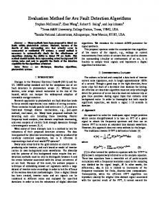
Current techniques of estimating high frequency (1 pixel) as well as sub-pixel image jitter. An image stabilization routine was developed to correct for the jitter by comparing the image to a reference image created for each time. The reference images is constructed using the closest image in time with a clear sky and scaling it for the correct intensity for that date and time. The detection of clear sky images is described in the next section. Images are aligned to the present reference image by first expanding each image’s resolution four times by linearly interpolating in both x and y dimensions. Correlation coefficients are calculated between the two images for each position with the expanded resolution image shifted by +/- 16 pixels in the x and/or y directions. The location with the highest normalized cross-correlation is chosen as the aligned image. Finally, the shifted image is transformed to the original resolution through bilinear averaging and antialiasing. With interpolation to higher resolution and image stabilization, both pixel and sub-pixel jitter were corrected to the reference image location. Fig. 3 demonstrates the necessity of performing image stabilization. This process was done using High Performance Computing parallel processing algorithms to simultaneously stabilize a large timeseries of images.

cloud detection using a threshold determined by the brightest pixel technique.

Fig. 3. Illustration of image stabilization algorithm: (a) image after jitter correction; (b) difference between original and reference image; (c) difference between aligned and reference image.

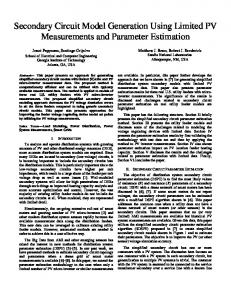
B. Cloud Detection Identification of visible clouds in the images is not a straightforward process. Challenges include (1) variation in average image intensity and image contrast with time of day and time of year due to the variable solar intensity and angle of the sun on the land surface and (2) variability of the brightness of different ground features, such as dry lake beds and snow, which can appear very similar to clouds. Two main methods were used for identifying clouds in the satellite imagery. The first method was thresholding the image based on simply finding pixels with intensity values above a certain threshold value. The clouds are more reflective than most geographical features, so especially certain types of clouds can be easily identified this way. Thresholding can be accomplished with a fixed threshold intensity value or with a moving threshold that depends, for example, on features within the image or the time of day. The thresholding method works better under some weather conditions than others. For example, cumulous clouds are easily distinguished from the background because they are the brightest features in the image, whereas broad thin stratus clouds are more difficult to distinguish from background. Fig. 4 shows an example of

Fig. 4. Example of Cloud Detection using Thresholding: raw image (left) and detected clouds (colored features, right).

The second method used for detecting clouds was Movement Detection. In this technique, the intensity is compared between pairs of sequential images at the pixel level. After scaling each image so that there was no average change in the brightness of the image, the difference in intensity exceeding a certain threshold was assumed to be movement at that pixel. With accurate jitter correction, the only features in the image that can move are clouds; therefore pixels with movement were assumed to be clouds. One problem with this method is that it can only identify leading and trailing edges of clouds. This is because a pixel may be in the middle of the cloud in both images and the difference

between intensity at these pixels may not exceed the threshold. Another problem with this method is that it depends on the accuracy of the image stabilization method, since errors in stabilization can lead to apparent movement of ground features and misidentification of these features as clouds. Fig. 5 shows an example of cloud detection using the movement detection technique, and illustrates the main problem with this method. Parts of the clouds recognized in the image are not identified as clouds by the movement detection technique. Note how the large cloud in the center of the image appears thinner in the movement detection image. Several shadows on the ground are also identified as clouds since they move between images.

an image would look like for any date for that location without clouds. The synthetic background images are verified to match the min, max, and mean intensity for each time and day of the year.

Fig. 6. Example satellite image with background subtraction for southern Nevada. Approximate state boundaries in yellow.

A. Determining Background Portion of the Image

Fig. 5. Example of Cloud Detection using Movement Detection: raw image (left) and detected clouds (white features, right).

V. BACKGROUND SUBTRACTION In order for the neural networks to learn the correlation between the clouds and the ground irradiance, the background image of the ground must be removed. This ensures that the neural network only models the impact of the clouds to the clearness index and not the geographical features. Background subtraction was accomplished by estimating what an image of the ground would look like and subtracting this image from the actual image. Areas with clouds should then show up as areas where the intensity difference is above a certain threshold. Fig. 6 shows an example of cloud detection by the method of background subtraction. Note how the background disappeared (i.e., is colored black) in the right panel of Fig. 6 and all that remains in the subtracted image are the clouds. This method allows for better detection of clouds with lower intensity because of less reflectivity. Even small changes in intensity can be detected between the image and the expected background. For example, with background subtraction a cloud pixel could be detected if it is just slightly brighter than normal, even if it is still darker than another geographical feature in the image. As a result of background subtraction, the subsequent image analysis depends only on the clouds in the image, and not on any of the background content. This method allows the ANN to learn the connection between cloud images and irradiance variability without the ground data included in the image. An additional ANN can be used to generate the background image that varies with the seasonal and daily changes. This ANN is automatically trained by detecting and using only images of the location without clouds throughout the year. It can then generate what

Background Subtraction requires determination of a background image without the presence of clouds. First, Movement Detection was used to select a subset from available images that contain no clouds. If any movement was detected the image was flagged as having clouds, and every day that had images with clouds was classified as a cloudy day. This high sensitivity in detecting clouds guarantees that only days that were completely clear are used to generate the background images. For each of the images with clear skies, image statistics (mean, minimum and maximum) of the pixel intensity are computed. These statistics vary in a smooth manner during daylight hours and in a more complex but non-random manner annually. Pixel intensity in an image of the background varies due to diurnal and seasonal changes in solar illumination. Because the background image varies by season and time of day, and clear sky images are not available at all times, a neural network that is trained on the clear images throughout the year was used to generate images for all other times during the year. B. Neural Network Learning of Clear Images Pixel intensities do not necessarily vary algebraically between clear sky images because of changes in earth’s albedo, the occurrence of snowfall, and atmosphere properties. In order to generate suitable background images of the ground for all times of interest, a neural network was developed and trained to produce reference background images. The feedforward backpropagation ANN was set up with two hidden layers of 300 neurons with a log-sigmoid transfer function. The BFGS quasi-Newton backpropagation algorithm in MATLAB was used to train the ANN with the detected clear day images. The ANN was trained to take the date and times as inputs and produce minimum, average, and maximum pixel values for any time when clear sky images were not available. This setup can be seen in Fig. 7.

synthetic image retains the general structure and characteristics evident in the GOES-11 image. Fig. 9b shows that the ANN also learned the diurnal variation through the year to account for different lengths of days and solar intensity. Clear Day (06/09/08)

Pixel Intensity

10000

Fig. 7. Training ANN to generate clear background images

C. Neural Network Generation of Clear Images

IB   IC   mean IC  max IC   min IC 

(1)

I t   I B I t,max  I t,min   I t,mean

(2)

Fig. 8 compares pixel intensities for synthetic images to those from images during clear sky days throughout 2008. The comparison shows that the neural network and scaling produced images for which the average pixel intensity follows the annual pattern.

Average Image Intensity

5000

0 0

ANN Output Clear Images

6000

5

10

15

20

Time (PST) Images Without Clouds

7000 Average Intensity

Once the ANN has been trained, for any input time t, it produces minimum (It,min), average (It,mean), and maximum (It,max) pixel values. Clear images for each day of the year were generated by scaling the pixels in the baseline image IB to the neural network generated statistics for every time t. The closest clear sky image, as determined by the cloud detection, was selected as the base reference image IC. The baseline image IC was normalized to IB using (1) to create an image that is easily scaled for any given time It. This resulting image It represents what the image would look like for a clear, cloudless sky at that time.

7000

Image Max Simulated Max Image Mean Simulated Mean Image Min Simulated Min

03/22/08 03/22/08 Sim 06/09/08 06/09/08 Sim 02/05/08 02/05/08 Sim

6000 5000 4000 3000 2000 4

6

8

10

12

14

16

18

Time (PST)

Fig. 9. Comparison of pixel intensity of clear sky images and ANN simulated output for a) Diurnal variation in image statistics and b) diurnal variation for different days of the year.

VI. TRAINING THE NEURAL NETWORK MODEL The ANN model was trained using measured ground irradiance between the two images 15 minutes apart. The irradiance was transformed to clearness index by dividing by the clear sky model irradiance. The feed-forward backpropagation ANN was set up with three hidden layers of 300 neurons with a log-sigmoid transfer function. The BFGS quasi-Newton backpropagation algorithm in MATLAB was used to train the ANN with the satellite images as inputs and the ground clearness index as the output as shown in Fig. 10.

5000 4000 3000 2000 0

50

100

150

200

250

300

350

Day Of Year

Fig. 8. Comparison of average pixel intensity of clear sky images and ANN simulated output through the year.

Moreover, for individual clear sky days, Fig. 9a shows the neural network was found to produce synthetic images which had statistics reasonably close to the statistics for the actual clear day images. Fig. 9a shows that the

Fig. 10. Training the Neural Network model to generate clearness index from background subtracted satellite images.

One week of images and data was used the train the ANN model. An example of the model learning the training data is shown in Fig. 11 where the model learned the correlation between the images and irradiance very accurately. Fort Apache NN Output

1200

Irradiance (W/m 2)

1000

800

600

400

Fig. 12. Measured and simulated (NN Output) irradiance for Fort Apache at 1 minute resolution for May 27, 2008.

200

0

0

100

200

300

400 500 600 Time (minutes)

700

800

900

1000

Fig. 11. Measured and simulated (NN Output) irradiance for Fort Apache at 1 minute resolution for May 25, 2008.

VII. RESULTS After the model has been developed using known ground irradiance values, it can be implemented anywhere with satellite images. The current hypothesis is that the trained ANN will only be able to work with similar weather patterns as in the training data, so it may only work for geographically similar locations with relatively similar weather and clouds. The simulation results will have to be verified with some of the sample sites used in the model development process and some new sites with minute irradiance data to compare the model accuracy for weather type. The correlation and residuals of the irradiance and variability can then be analyzed. Current model results can be seen in Fig. 12 for Fort Apache for the week after the training data. The model very accurately models the large transitions of the cumulous clouds later in the day, but has more trouble with the variability produced from the high thin cirrus clouds earlier in the day.

ACKNOWLEDGEMENT Sandia National Laboratories is a multi-program laboratory managed and operated by Sandia Corporation, a wholly owned subsidiary of Lockheed Martin Corporation, for the U.S. Department of Energy’s National Nuclear Security Administration under contract DE-AC04-94AL85000.

VIII. CONCLUSION A proof of concept model was developed to predict high frequency irradiance variability in areas with no ground sensors. Artificial Neural Networks (ANN) can be used to generate clear background images to do background subtraction, cloud identification, and cloud classification in satellite imagery. The ANN model has difficulty modeling all possible images to irradiance patters, but categorizing clouds and using separate neural networks for each cloud type could improve accuracy. The overall processing is very intensive and utilizing High Performance Computing Resources is necessary. For interconnection studies modeling solar power on the electric grid, a good model for system variability is needed. This method shows the possibility of modeling highresolution solar variability using only satellite images. REFERENCE [1] NOAA. (2010, July). NOAA's Comprehensive Large Array-data Stewardship System. Available: http://www.class.ngdc.noaa.gov/saa/products/welcome [2] R. Perez, P. Ineichen, K. Moore, M. Kmiecik, C. Chain, R. George, and F. Vignola, "A new operational model for satellite-derived irradiances: Description and validation," Solar Energy, vol. 73, pp. 307-317, 2002. [3] 3TIER. (2011, Feb.). 3TIER: Renewable Information Services. Available: http://www.3tier.com [4] J. S. Stein, A. Parkins, and R. Perez, Validation of PV performance models using satellite-based irradiance measurements : a case study, 2010.