Neuron, Vol. 37, 989–999, March 27, 2003, Copyright 2003 by Cell Press
Pyramidal Neuron as Two-Layer Neural Network
Panayiota Poirazi,1,* Terrence Brannon,2 and Bartlett W. Mel3,* 1 Institute of Molecular Biology and Biotechnology Foundation for Research and Technology, Hellas (FO.R.T.H.) Vassilica Vouton P.O. Box 1527 GR 711 10 Heraklion, Crete Greece 2 Metaperl IT Consulting 135 Corson Avenue Staten Island, New York 10301 3 Department of Biomedical Engineering and Neuroscience Graduate Program University of Southern California Los Angeles, California 90089
Summary The pyramidal neuron is the principal cell type in the mammalian forebrain, but its function remains poorly understood. Using a detailed compartmental model of a hippocampal CA1 pyramidal cell, we recorded responses to complex stimuli consisting of dozens of high-frequency activated synapses distributed throughout the apical dendrites. We found the cell’s firing rate could be predicted by a simple formula that maps the physical components of the cell onto those of an abstract two-layer “neural network.” In the first layer, synaptic inputs drive independent sigmoidal subunits corresponding to the cell’s several dozen long, thin terminal dendrites. The subunit outputs are then summed within the main trunk and cell body prior to final thresholding. We conclude that insofar as the neural code is mediated by average firing rate, a twolayer neural network may provide a useful abstraction for the computing function of the individual pyramidal neuron. Introduction The neuron-like unit most often used in models of brain function over the past 50 years is the classical “point neuron,” in which a weighted sum of synaptic inputs from across the cell is passed through a single spikegenerating mechanism near the cell body (McCullough and Pitts, 1943; Rosenblatt, 1962; Rumelhart et al., 1986). From a modern perspective, however, the point neuron seems likely to be a poor model of synaptic integration in cells with large, profusely branched, active dendritic trees. In keeping with the idea that a dendritic arbor might support a moderately large number of independent nonlinear operations (Llina´s and Nicholson, 1971; Koch et al., 1982; Rall and Segev, 1987; Shepherd and Brayton, 1987; Mel, 1992b, 1992a, 1993), evidence from anatomical, physiological, and modeling studies *Correspondence:
[email protected] (P.P.),
[email protected] (B.W.M.)
(Ha¨usser et al., 2000; Segev and London, 2000; Stuart et al., 1999) led us to argue previously for a two-layer model of synaptic integration in pyramidal cells (Mel et al., 1998; Archie and Mel, 2000; Poirazi et al., 2003 [this issue of Neuron]). According to this idea, spatially restricted domains within the dendritic tree act as separately thresholded functional “subunits” and provide the cell’s first layer of internal computation (Schiller et al., 2000; Wei et al., 2001). In the second layer, the subunit outputs are summed and then thresholded to produce the cell’s overall response. Assuming that all inputs to the cell are either 1 or 0, i.e., active or inactive, and that all synaptic weights are of unit size, the cell’s hypothetical input-output function can be expressed as y⫽g
冤 兺 ␣ s(n )冥, m
i
i
i⫽1
where ni is the net number of excitatory synapses driving the ith subunit, s(n ) is the subunit input-output function, ␣i is the weight on the ith subunit, m is the number of subunits in the cell, and g is a global output nonlinearity (Figure 1A). In previous work using a simple “ball and sticks” model of a neocortical pyramidal cell (Archie and Mel, 2000), we found that when a total of 16 excitatory synapses were placed on two identical cylindrical branches connected to the soma, the cell’s output firing rate approximated a sum-of-squares law, that is, with s(n ) ⫽ n2 and ␣i ⫽ 1, giving y ⫽ g(n12 ⫹ n22). The finding was intriguing given the frequent appearance of squaring nonlinearities, as in “energy models,” and pairwise multiplicative nonlinearities, as in “gain fields,” in diverse models of cortical receptive field structure (Adelson and Bergen, 1985; Zipser and Andersen, 1988; Peterhans and von der Heydt, 1989; Heeger, 1992; Kapadia et al., 1995; Ohzawa et al., 1997; McAdams and Maunsell, 1999; Salinas and Thier, 2000; Chance et al., 2002). It was unclear, however, whether the simple sumof-squares form would also predict the firing rate of a realistic pyramidal cell morphology containing a full complement of active dendritic channels, especially under the more varied stimulus conditions likely to exist in vivo. In addition, studies of subthreshold synaptic integration have been suggestive of a sigmoidal, rather than squaring, subunit nonlinearity (Schiller et al., 2000; Wei et al., 2001). This leaves open the important questions as to (1) which physical subregions of a dendritic arbor can act as independent functional subunits and (2) which subunit i/o function, whether linear or nonlinear, accelerating or saturating, might best represent the cell’s integrative behavior when it is driven to fire at high rates. To address these questions, we developed a compartmental model of a CA1 pyramidal cell within the NEURON simulation environment (Hines and Carnevale, 1997), among the most detailed single-cell models ever constructed. In lieu of a uniform low concentration of classical Hodgkin-Huxley-type sodium and potassium channels in the dendritic membrane as was used in
Neuron 990
here we drove from 32 to 63 excitatory synapses on 4 to 37 thin dendrites emanating from the apical trunk over a 350 m range, some branches connected directly to the main trunk, others with one or two intervening branch points. We also drove the cell with an extremely varied, spatially heterogeneous set of synaptic activation patterns and quantitatively compared the predictive power of Equation 1 with four different subunit nonlinearities, including s(n ) ⫽ n2, n3, 公n, and a sigmoidally modulated function of the form 1/(1 ⫹ exp(( ⫺ n)/s )) ⫹ an ⫹ bn2 (Figure 1B). As our “null hypothesis,” we tested the single-layer point neuron model which follows from the assumption of a linear subunit function s(n ) ⫽ n. Results We began with the assumption that the dendritic subunits of the CA1 pyramidal cell correspond physically to the several dozen long, thin, unbranched, terminal dendrites of the apical and basal tree that together receive 85% of the excitatory synaptic input to these cells (Megı´as et al., 2001). The experiments reported here have focused on synaptic integration within the thin branches of the apical tree, since these branches, with their considerable variation in distance from the cell body, represent the severest challenge to any simple two-layer abstraction of the neuron’s input-output behavior. The assumed mapping between thin dendrites and the subunits of a two-layer network model is shown schematically in Figure 1A. Figure 1. Pyramidal Neuron as Two-Layer Neural Network (A) Hypothetical mapping between thin terminal branches and independent subunits of a two-layer neural network. Subunit weights ␣i are shown as filled circles. (B) Five candidate subunit functions s(n ) were evaluated as predictors of the compartmental model’s mean firing rate. The formula for the sigmoid curve is s(n ) ⫽ 1/(1 ⫹ exp((3.6 ⫺ n )/0.20) ⫹ 0.30n ⫹ 0.0114n2.
Archie and Mel (2000), the present model contained 17 types of voltage-dependent ion channels whose biophysical properties and nonuniform spatial distributions were culled from published experimental studies, in addition to four types of synaptic conductances which were used to drive the cell (see Experimental Procedures). The model replicates a wide range of data from in vitro physiological studies, including input and transfer resistances in the apical trunk and their dependence on Ih, the contributions of IA and Na⫹-channel inactivation to the attenuation of back-propagating action potentials, the varying threshold for Ca2⫹ spike initiation along the soma-dendritic axis, and the location-dependent rules governing summation of paired EPSPs (see the Supplemental Data available online at http://www. neuron.org/cgi/content/full/37/6/989/DC1 and Poirazi et al., 2003). The realistic cell morphology used in these experiments presented a severe challenge to the idealized two-layer network hypothesis expressed by Equation 1. In lieu of stimulating two identical uniform branches protruding from a spherical soma (Archie and Mel, 2000),
Generating a Rich Stimulus Set A set of 1000 synaptic stimulus patterns was constructed so that over the ensemble (1) any given branch could be activated at a range of intensitities (from 0 to 9 excitatory synapses); (2) any given trial could include a small number of strongly activated branches (as few as 4), a large number of weakly activated branches (as many as 37), or any mixture of a small, medium, or large number of branches with weak, intermediate, or strong activation; and (3) the total amount of excitatory synaptic drive could vary significantly over the set of trials (from 32 to 63 total excitatory synapses). To achieve this, we distributed excitatory synapses as follows. A number of excitatory synapses e was first chosen with e 僆 {32, 35, 36, 40, 45, 48, 49, 63} for distribution onto the apical dendrites. To illustrate for the case of e ⫽ 40 synapses, a number c was chosen between 0 and 5, and c branches were selected at random from the 37 thin terminal sections in the apical tree. Each selected branch received eight excitatory synaptic contacts, representing a strong stimulus to that branch. All other (40 ⫺ 8c ) synapses were distributed at random onto all other (37 ⫺ c ) branches in the set. In most cases, the remaining excitatory synapses were widely dispersed and occurred alone on their respective branches. In a second set of runs, a number c was again chosen between 0 and 5, and c randomly chosen branches received six excitatory synapses, and c other branches received two synapses each. All remaining synapses were again distributed at random onto all other branches in the set. In a third set of runs, 2c randomly
Pyramidal Neuron as Two-Layer Neural Network 991
Figure 2. Responses to High-Frequency Synaptic Stimulation Shown for Three Cases with 40 Excitatory Synapses Distributed across the Apical Tree In a fully dispersed case (left column), all 40 synapses were randomly assigned to the 37 terminal branches. In a fully concentrated case (right column), synapses were placed eight to a branch on five randomly chosen branches. Heterogeneous cases consisted of randomized assignments of one, two, four, six, or eight synapses to varying numbers of terminal branches. Middle column shows a case with two groups each of two (blue) and six (yellow), plus 24 randomly dispersed synapses (green). Excitatory synapses were distributed at equally spaced intervals on each branch according to the formula pos(i ) ⫽ (2*i ⫺ 1)/(2*nsyns), where the distal end of the branch corresponds to pos ⫽ 1. Other placement schemes including random distribution within the branch were tried with similar results. A fixed set of 11 inhibitory synapses was used in all runs, including five at the cell body (3 nS for GABAA and 0.005 nS for GABAB) and six inhibitory synapses at ⵑ60 m intervals along the main trunk (2.4 nS for GABAA and 0.5 nS for GABAB). In runs containing more than 40 excitatory synapses, an additional GABAA conductance (equal to the AMPA conductance value) and a GABAB conductance (equal to 60% of the AMPA conductance value) was placed in the middle of each distal apical tip more than 350 m from the cell body (six tips). (A)–(C) show recording sites and corresponding responses in trunk and cell body. Somatic spike counts were recorded over 600 ms, for comparison with predictions of the abstract two-layer model with various choices for the subunit function s(n). Cell morphology was “n123” from the Duke/Southampton archive of neuronal morphology at http://www.cns.soton.ac.uk/ⵑjchad/cellArchive/cellArchive.html (Cannon et al. 1998).
chosen branches received four excitatory synapses, and all remaining synapses were distributed at random. Ten trials were run for each value of c for each of the three distribution schemes (8s, 6 ⫹ 2s, and 4 ⫹ 4s), leading to a total of 180 runs. A similar distribution strategy was used for the other values of e, leading to an overall stimulus set with e ⫽ 32 (distributing 8s, 4 ⫹ 4s and 6 ⫹ 2s, giving 150 stimuli), e ⫽ 35 (distributing 5s and 7s, giving 140 stimuli), e ⫽ 36 (distributing 6s, giving 70 stimuli), e ⫽ 40 (distributing 8s, 4 ⫹ 4s and 6 ⫹ 2s, giving 180 stimuli), e ⫽ 45 (distributing 5s and 9s, giving 160 stimuli), e ⫽ 48 (distributing 6s, and 8s, giving 160 stim-
uli), e ⫽ 49 (distributing 7s, giving 80 stimuli), and e ⫽ 63 (distributing 7s and 9s, giving 180 stimuli). Eighty of the 140 redundant cases with c ⫽ 0 were eliminated, leaving 1030 runs total. To facilitate formation of even groups for cross validation runs, 30 additional stimuli were randomly eliminated from the set, leaving exactly 1000 stimulus patterns. Excitatory synapses contained both NMDA and AMPA-type conductances with peak values in a ratio of 2.5 to 1. The absolute magnitudes of the synaptic conductances were scaled in pilot runs to yield a 5mV peak EPSP locally at each synapse; this facilitated auto-
Neuron 992
Figure 3. Local and Somatic Responses to 50 Hz Independent Poisson Trains Delivered to 3, 7, or 11 Excitatory Synapses Separate experiments are shown for two apical tip dendrites at 212 m (thick traces) or 355 m (thin traces). Distance to cell body was measured from nearest point of intersection with apical trunk, projected perpendicularly down the main axis of the cell to the level of the soma. Mean depolarization v is shown next to each somatic trace.
matic generation of a large set of runs with reasonable postsynaptic voltage ranges. Examples of three different stimulus configurations with e ⫽ 40 excitatory synapses are shown in Figure 2, leading to output firing rates ranging from 3 to 36 Hz. Measuring the Branch Coupling Coefficients To compare firing rates generated by the biophysical model to those predicted by the abstract model of Equation 1, it was necessary to determine the values of the coefficients ␣i representing the strength of each branch’s coupling to the cell body. For each of the 37 target branches in the apical tree, we used two different methods for determining the coupling coefficients. In the simpler “direct” method, a separate set of pilot experiments was carried out in which each branch was stimulated individually with varying numbers of excitatory synapses driven by independent 50 Hz Poisson trains for 250 ms. Example recordings from two branches stimulated in separate experiments with either n ⫽ 3, 7, or 11 excitatory synapses are shown in Figure 3, along with simultaneously recorded somatic traces. A clear local input-output nonlinearity is evident in these traces, insofar as equal increments in stimulus intensity (3 → 7 → 11 active synapses) leads to unequal increments in the intensity and quality of the local compartment response: only at higher stimulus intensities and longer delays do large voltage-dependent NMDA, Na⫹, and Ca2⫹ currents begin to contribute heavily to the local voltage response (Schiller et al., 2000; Wei et al., 2001). Mean depolarization at the cell body is indicated next to each somatic trace. The different form of the local voltage traces in the two stimulated dendrites, as evidenced by the unequal prominence of fast versus slow spikes at higher stimulus intensities, is a reflection of the nonuniform spatial distribution of several channels as a function of distance from the cell body. These in-
clude an elevated density of Ca2⫹ and persistent Na⫹ current coupled with a lower concentration of Ca2⫹dependent K⫹ channels distally and a reduction in slow Na⫹ channel inactivation in the most distal apical tips. The combined effects of these inhomogeneities is to lower the threshold for Ca2⫹ spike initiation in the distal apical arbor (Amitai et al., 1993; Golding et al., 1999). In spite of these biophysical inhomogeneities, all branches were treated identically in the direct procedure used to determine the ␣i values. For each branch, the mean somatic depolarization vi(n ) over the 250 ms run was recorded for n ranging from 1 to 10 excitatory synapses, and ␣i was set to the mean value of vi over the set of runs, that is, ␣i ⫽ 1/11⌺10 n ⫽ 0 vi(n), with vi(0 ) ⫽ 0. Directly determined ␣i coefficients are shown graphically in the top plot of Figure 4. The strength of coupling—shown in arbitrary units—varied relatively little with distance to the soma, owing to the greater propensity for calcium spiking in the distal apical tree which helped to counteract the distance-dependent attenuation of signals traveling to the cell body (Cauller and Connors, 1992). However, the coefficient magnitudes were more clearly tied to branch order: first-order thin dendrites (connected directly to the trunk and shown in red) exerted a more powerful influence on the cell body—about 40% more on average—than dendrites that were one or more branch points removed (shown in blue). Mean coefficient values within each group are shown as asterisks on the right-hand vertical axis in each plot. The second method used to determine the branch coupling coefficients involved a least mean squared error (LMS) procedure, which optimized the parameters of the abstract model of Equation 1 to best predict the actual firing rates of the biophysical model over the 1000 pattern stimulus set. Coefficients optimized for sigmoidal branch subunits were similar to those deter-
Pyramidal Neuron as Two-Layer Neural Network 993
Figure 4. Determining Couplings between Thin Branches and Cell Body (Top) First-order branches (in red) were those connected directly to the apical trunk (shown in heavy black); second- and higher-order branches are shown in blue. Schematic representation of pyramidal cell soma was added for clarity. Graphs show numerical coupling strength ␣i as a function of perpendicular distance from the base of the branch to the soma; pairs of sister branches lie at the same distance. Coefficients were determined either by direct measurement of electrical coupling between branch and soma (top plot) or by LMS fits of actual firing rates generated by the biophysical model to those predicted by the abstract model of Equation 1 with either sigmoidal (middle plot) or linear (lower plot) subunits. In each case, LMS fits optimized the 37 coupling coefficients ␣i and the three parameters of the output sigmoid. For the middle plot, the four parameters of the branch sigmoid were also optimized. All 1000 data points were used in the fitting procedure since multiple leave-10%-out cross validation runs indicated that overfitting was not an issue. Mean values of coefficients within each group are shown as asterisks on the vertical axis at the right in each plot. Coefficients were normalized within each plot so that the mean higher-order branch coefficient was 1. Coefficients determined by LMS error minimization with sigmoidal branch subunits (middle plot) were similar to those determined by direct parameter-free measurement of branch-tosoma couplings (top plot).
mined by the parameter-free direct method (compare top and middle plots in Figure 4) but showed slightly greater variance as well as a slightly greater difference between coefficients for first- versus higher-order branches. Like the directly measured coefficients, optimized coefficients showed virtually no dependence on distance from the soma, supporting the idea that the apical tree is more democratic than its spatially extended morphology superficially suggests (Magee and Cook, 2000). Coefficients optimized for linear subunits are shown in the lower plot of Figure 4. While clearly correlated with the other two sets, the linear subunitoptimized coefficients covered a much larger dynamic range including several coefficients near zero, and exhibited greater overlap in the distribution of first- (red) and higher-order (blue) branch coefficient values. Predicting Responses to Complex Patterns of Synaptic Stimulation Having estimated coupling coefficients for each branch, we used Equation 1 to predict the cell’s output firing rate in response to each of the 1000 complex stimulus patterns. In effect, we sought to determine whether a very simple mathematical expression could accurately predict the behavior of a very complicated biophysical model, the former involving essentially a “paper and pencil” calculation, the latter involving numerical integration of thousands of coupled nonlinear differential equations through thousands of time steps. For each stimulus pattern, we first compared the average firing
rate of the cell to the predictions of Equation 1 using LMS-optimized branch coefficients. Separate predictions were generated for each of the five candidate subunit functions shown in Figure 1B. Prediction results for the entire data set are shown in the scatter plot of Figure 5 for the best-performing nonlinear subunit function in blue—the sigmoid—and for the linear subunit function in red. Output sigmoid parameters were optimized per choice of subunit function as a part of the overall LMS fitting procedure, incidentally leading to nearly identical output functions for linear and sigmoid subunits (and only three different basic shapes overall—see inset and caption of Figure 5). The correlation between predicted and actual firing rates using sigmoidal subunits was very high (r2 ⫽ 0.94), indicating that for the set of synaptic activity patterns contained in the overall stimulus set, the two-layer sumof-sigmoids network provided an excellent model of the pyramidal neuron’s average firing rate. Contrary to expectation, however, the correlation between predicted and actual firing rates using linear subunits, though lower, was still quite high (r2 ⫽ 0.82). This indicated that variation within the set of stimulus patterns we used to drive the cell led to variation in output firing rates that was in large part predictable by a (linear) point neuron. Distinguishing Power versus Configuration Variation The comparable power of linear and nonlinear subunits in predicting the overall stimulus set highlighted the
Neuron 994
Figure 5. Correlation between Predicted and Actual Firing Rates for Abstract Model Neurons with Either Linear or Sigmoidal Subunits Scatter plot shows results for all 1000 stimulus patterns. The abstract two-layer model with sigmoidal subunits explains 94% of the spike rate variance generated by the biophysical model. In comparison, the linear (point neuron) model captures 82% of the spike rate variance. Inset: Optimized output sigmoids for the five different subunit functions tested. Parameters of the output sigmoid were nearly identical for linear and sigmoid subunit choices, g(x ) ⫽ 0.96*x./(1 ⫹ 1509*exp(⫺0.26*x)); for s(n ) ⫽ n2, the optimal output sigmoid was g(x ) ⫽ 1.10*x./(1 ⫹ 565*exp(⫺0.59*x)), and for s(n ) ⫽ n3 and s(n ) ⫽ 公n, the optimal output function was a straight line.
need to distinguish variation in the stimulus set that is accessible to a linear model, which we term power variation, from variation that is inaccessible to a linear model, which we term configuration variation (Figure 6A). Power variation corresponds to varying projections of input patterns onto the weight vector of the optimal linear model, i.e., variation in the quantity n·␣Linear. In practical terms, power variation in the stimulus set results from different numbers of excitatory synapses used to drive the cell and/or from variation in the number of synapses targeting strongly or weakly coupled branches. Intuitively, a linear model can capture the fact that a cell driven by 60 synapses will fire more spikes on average than a cell driven by 30 synapses and that a cell driven with 50 synapses on strongly coupled branches will fire more than a cell driven by 50 synapses on weakly coupled branches. Configuration variation is defined as all variation in the stimulus set that is not power variation. Nearly pure configuration variation can be found within any set of stimulus patterns with nearly equal projections onto the vector ␣. In Figure 6A, nearly equal power (NEP) stimulus sets correspond to the gray strips in the input space oriented perpendicular to ␣. For every pattern contained within an NEP strip—which is actually a 36 dimensional linear subspace—the linear-subunit model generates nearly the same output prediction. Any variation in actual firing rates for the different patterns within such a stimu-
lus set—corresponding to undulations in the purple strips in Figure 6A—was therefore due to changes in stimulus configuration and lay outside the representational scope of the linear model. Intuitively, configuration changes correspond to different spatial arrangements of an approximately constant number of excitatory synapses. Ten groups of NEP stimuli were formed from the overall data set by sorting the 1000 complex stimulus patterns along the power axis, i.e., according to the magnitude of the predictions of the best linear model. The data were then divided along the power axis into ten groups of 100 patterns each. Groups 1, 5, and 8 are shown in Figure 6B, each within its own vertical red dashed box. The ten groups of NEP stimuli were analyzed separately to calculate how much of the variability in actual firing rate within each box could be explained by Equation 1 using different choices for the branchsubunit function s(n ). Given the non-zero thickness of the NEP data sets along the power axis, the linear model would be expected to retain a small modicum of predictive power. On average, the sigmoidal subunit function explained 67% of the spike rate variance within the ten NEP data sets, as compared to 11% for the linear model. The three NEP data sets shown in blue boxes in Figure 6B correspond pattern-for-pattern to the data in the adjacent red boxes, except that the data in blue boxes are arrayed along the x axis using predictions of the sigmoid model rather than the linear model. The fraction of variance explained (r2 ) within each NEP set is shown next to each box. Thus, in contrast to what we found for the overall stimulus set, which was dominated by power variation, in NEP data sets where configuration variance dominates, sigmoidal subunits predict six times more variance in the spike rate data than do linear subunits. Performance figures for all five subunit functions on the ten NEP data sets are shown in Table 1. After the sigmoid function, the second-best subunit nonlinearity n2 captured only 36% of the configuration variance in these same data sets. Since the choice of NEP data sets guaranteed that the linear model would perform badly, it was crucial to determine whether the superior predictive power of sigmoidal subunits would hold for other kinds of nearly equal prediction data groupings. In particular, if the data were analyzed in nearly equal prediction groups for the optimal sigmoid subunit model, which would guarantee its poor performance, would other subunit choices lead to better predictive power? As shown in columns 4–8 of Table 1 under the heading “Nearly Equal Prediction Groupings,” sigmoidal subunits outperformed all other choices of subunit function regardless of how the data were grouped, whether sorted by near equal predictions of the abstract model with s(n ) ⫽ n, sigmoid(n ), n2, n3, or 公n. This can be seen by comparing each bold value—the spike rate variance explained by sigmoidal subunits—to all other values in the same column. Values in parentheses along the diagonal arise from data groupings designed to be maximally disadvantageous to the model in question. This handicapping of each model in turn was borne out in the prediction results, with two exceptions: (1) when stimuli
Pyramidal Neuron as Two-Layer Neural Network 995
Figure 6. Prediction Performance of Linear versus Sigmoidal Subunit Models for Nearly Equal Power Stimulus Groups (A) Geometry of power versus configuration variance in the stimulus set. The horizontal plane represents 37 dimensional input space indexed by n ⫽ {n1, . . ., n37}, with ni representing the number of excitatory synapses active on branch i. Stimulus patterns are represented by black dots in the input space; those contained within gray shaded boxes have nearly equal power (NEP), i.e., nearly equal projections onto the weight vector ␣ of the optimal linear model. The yellow surface schematically represents the true neural response function with firing rate on the vertical axis. The cyan hyperplane shows the best-fitting linear model, with equi-response contours running perpendicular to ␣. Magenta strips represent actual firing rates for input patterns within NEP stimulus groups; spike rate variance within each (nonplanar) strip lies mostly outside the representational scope of the (planar) linear model. For graphical clarity, effects of the output nonlinearity g have been omitted. (B) Comparison of predictions of abstract models with either linear (red) or sigmoidal (blue) subunits for three of the ten NEP stimulus groups. Each red box contains scatter data for 100 stimuli with nearly equal projections onto ␣, hence the narrow spread along the x axis. Shading indicates conceptual connection to NEP regions in the input space as shown in (A). Pairs of corresponding (adjacent) red and blue boxes contain identical sets of 100 stimulus patterns with one-to-one matching of actual firing rates but plotted against predictions of either the abstract linear (red) or sigmoid (blue) subunit models. Predictions using sigmoidal subunits capture far more spike rate variation for NEP stimulus groups; r2 values are shown next to each box.
were grouped according to similar predictions of the linear model, the 公n subunit was actually the worst performer (the linear model was second worst), and (2) when stimuli were sorted by predictions of the sigmoid model, the sigmoid model still predicted better than all the others. This suggests that the configuration variation that is inaccessible to a two-layer model with sigmoidal subunits is inaccessible to any model expressed in the simple form of Equation 1. Sigmoidal subunits also predicted output spike rates
better than any other subunit function on a stimulus set containing a nearly pure form of power variation: the set of 80 stimulus patterns with varying numbers of excitatory synapses scattered diffusely across the apical tree. An example of this kind of stimulus is shown in the left column of Figure 2. Prediction performance for diffuse stimuli is shown in column 3 of Table 1 for each of the five-subunit functions tested. The superior prediction performance of the abstract two-layer network model with sigmoidal subunits was
Table 1. Prediction Performance Using Optimized Branch Coefficients Nearly Equal Prediction Groupings s(n)
All Stimuli
Diffuse
n
sigmoid(n)
n2
n3
公n
n sigmoid(n) n2 n3 公n
0.82 0.94 0.72 0.49 0.29
0.80 0.94 0.77 0.42 0.71
(0.11) 0.67 0.36 0.21 ⫺0.15
0.09 (0.16) 0.06 0.04 0.06
0.49 0.72 (0.08) 0.23 0.31
0.67 0.84 0.59 (0.04) 0.39
0.78 0.91 0.73 0.55 (0.03)
Values shown are the fraction of spike rate variance explained (r2 ) by the abstract neuron model of Equation 1 for the five subunit functions shown in Figure 1B. Values under the heading “Nearly Equal Prediction Groupings” are averaged over ten cohorts of 100 stimulus patterns sorted by prediction using the subunit function at the head of each column. All values were computed using LMS-optimized model parameters, including the 37 branch coefficients, parameters of s(n ) (if applicable), and parameters of the output sigmoid. The negative value indicates negative original correlation coefficient. Values in parentheses arise from data groupings designed to be maximally disadvantageous to the corresponding subunit function. Values for sigmoidal subunits are shown in bold to facilitate comparisons within each column.
Neuron 996
Table 2. Spike Rate Predictions Using Directly Measured Branch Coefficients NEP Groupings s(n)
All Stimuli
Diffuse
n
sigmoid(n)
n sigmoid(n)
0.69 0.90
0.87 0.92
(0.06) 0.67
0.09 (0.15)
Entries show percent of spike rate variance (r2 ) explained by Equation 1 for linear and sigmoidal subunit functions. Data format is the same as in Table 1.
not due to overfitting using the additional parameters contained within the branch sigmoid function. Overfitting was ruled out using a bootstrapping test in which the six branch sigmoid parameters were optimized with repeated leave-10%-out cross validation runs. No significant difference was observed between prediction performance for trained versus untrained patterns. Since overfitting did not occur and the prediction performance of sigmoidal subunits was superior to that of any other subunit function tried (particularly for spatial configuration variance), it is safe to infer that the sigmoidal branch nonlinearity captures bona fide structure in the inputoutput relation of the biophysical model cell. Interestingly, prediction performance of the abstract neuron model benefited only modestly from the LMS optimization of branch coupling coefficients. When the 37 branch coefficients were obtained—not by fitting models to the spike rate data, but by direct measurement of electrical coupling between each branch and the cell body (see Figure 3)—prediction performance was only modestly degraded on the data set as a whole: the fraction of variance explained dropped to 90% from 94% for the sigmoid model and to 69% from 82% for the linear model (Table 2). Furthermore, for the ten NEP data sets, which were dominated by variation in synaptic configuration, prediction performance for both linear and sigmoid models scarcely depended at all on optimized branch coefficients. This suggests that optimization of branch weights primarily helped the abstract models to cope with power variation in the stimulus set, rather than configuration variation. Since a neuron is likely to experience significant background activation in vivo, we tested whether the quality of the firing rate predictions generated by the abstract two-layer model would be influenced by manipulations designed to mimic background activation of the biophysical model cell. Using an earlier version of the biophysical model with slightly different stimulus and prediction protocols (including more inhibitory synapses, fewer stimulus patterns, and nonoptimized branch weights), we imposed a 10-fold reduction in Rm in all thin branches of the apical tree—designed to mimic the membrane shunting associated with strong background activation of the cell—coupled with a cell-wide 5mV upward shift in resting potential (to ⫺65mV). Together these biophysical manipulations had a negligible effect on prediction quality for both the linear and sigmoidal subunit models. Using this same earlier version of the model, we also tested whether prediction quality depended on our assumption of asynchronous input trains. To do this, we ran a stimulus set with 50 excitatory
synapses driven by synchronous 50 Hz Poisson input trains. Under these conditions, the cell was driven by a sequence of powerful cell-wide impulses arriving every 20 ms on average. Given that synchronization worked against the assumption of subunit independence implicit in the sum of Equation 1—see also discussion surrounding Figure 3D in Poirazi et al. (2003)—prediction quality was in this case significantly degraded, to 78% of the variance explained down from 91% for sigmoidal subunits using this version of the model. However, we did not rule out the possibility that a two-layer model with differently calibrated subunit and output sigmoids could accurately predict the cell’s firing rate under synchronous input conditions as well.
Discussion The nature of synaptic integration in pyramidal cells remains a question of great importance, which can ultimately be settled only by direct empirical investigation. Given the technical difficulties facing current experimental approaches, however, we have used a realistic biophysical model to search for a simplifying abstraction of a pyramidal cell, in the hope that our “model of the model” may facilitate future efforts to understand the computing functions of cortical tissue. We have found that the firing rate of a pyramidal cell in response to a diverse set of synaptic input patterns, involving dozens of high-frequency-activated synapses scattered about the dendritic tree, can be modeled by a simple equation, which happens to also describe a conventional twolayer feedforward neural network with sigmoidal “hidden” units. It is remarkable that, although the detailed cell model includes 21 types of ionic and synaptic channels and exhibits complex nonlinear dynamics, which vary with dendritic location and contain structure at many time scales, the cell’s final common output can be accurately predicted by a paper-and-pencil calculation that relies on just the few parameters needed to describe the subunit and output sigmoids. It is important to note, however, that predictions of the two-layer sigmoidal network model leave fully one third of the spike rate variance unexplained in NEP stimulus sets. Even on the full stimulus set, for which sigmoidal subunits explain 94% of the spike rate variance, on any given trial, predictions are far from perfect. For example, predictions of ⵑ20 Hz were associated with actual firing rates ranging from 10 to 30 Hz (see vertical span of blue circles for 20 Hz predictions in Figure 5A). These prediction “failures” could arise from factors such as randomness in the input spike trains or, more interestingly, from violations of the key assumptions underlying Equation 1. Specifically, a single subunit function may not be adequate to describe the input-output behavior of all 37 target branches in the apical tree. Moreover, subunit outflows may not sum strictly linearly but may interact in more complex ways. Distal subunits, for example, might multiplicatively boost the effectiveness of proximal subunits, a hypothesis we have not yet tested. In short, larger stimulus sets and more sophisticated abstract models will be needed to more fully characterize the biophysical model’s response behavior.
Pyramidal Neuron as Two-Layer Neural Network 997
Stimulus Sets, and How to Choose Them The dramatic variation in prediction quality for any given subunit function—compare values within any given row of Table 1—highlights the fact that the choice of stimuli can strongly bias the contest among simple abstract models competing to explain the firing rate behavior of the detailed biophysical neuron. As previously noted, both the linear-subunit and sigmoid-subunit models are very good performers on the overall stimulus set (Table 1). However, this observation does not imply that the biophysical model cell is “just as much a point neuron as a two-layer sum-of-sigmoids neural network.” To consider an extreme case of stimulus selection, if the stimulus set were chosen to consist only of patterns containing exactly 50 active synapses scattered diffusely on the second-order branches of the apical tree, the firing rate of the biophysical model cell would likely be well described by a constant value—a rather uninteresting portrait of the cell’s input-output behavior. To reject the hypothesis that the pyramidal cell is fundamentally a point neuron, therefore, we required stimulus sets which fell explicitly within or outside the representational scope of a thresholded linear neuron. This requirement motivated the distinction between power and configuration variation and led to the development of NEP stimulus sets. We found that, under conditions of relatively constant overall stimulus intensity, the two-layer model with sigmoidal subunits roundly outperforms the point neuron model and every other nonlinear subunit function tested. It remains an open question what kind of functionally relevant stimulus variation actually confronts a pyramidal cell in the CA1 region of the hippocampus or elsewhere. If the primary role of the pyramidal cell is to rate overall stimulus power, i.e., to fire in proportion to the number of active afferents impinging on its dendrites, then our findings suggest that the pyramidal cell can emulate a point neuron and carry out this relatively simple computational task. If instead the pyramidal neuron is asked to distinguish among a large number of different patterns of synaptic activation of similar overall intensity, a task beyond the grasp of a point neuron, then our findings suggest that the pyramidal cell can emulate a two-layer sigmoidal neural network and satisfy this more demanding requirement as well. In short, different simplifying abstractions may apply in different neural contexts. Finding the True Branch-Subunit Function We set out to determine the optimal form of the thinbranch subunit function under the two rather strong assumptions of Equation 1: that all subunits must share a single i/o function and that subunit outflows from across the apical tree must combine additively to influence the cell’s output firing rate. (Neither of these assumptions is likely to be strictly true, either for the biophysical model or for a real pyramidal neuron). Under these assumptions, nonetheless, we found that sigmoidally modulated subunit functions consistently outpredicted all others, especially for stimulus sets that emphasize configuration variance as shown in Figure 6. We achieved the best overall prediction performance using the relatively weak sigmoidal modulation shown
in Figure 1, though performance remained quite high for other more conventional S-shaped functions with sharper thresholds and more pronounced saturation. For the conventional sigmoid s(n ) ⫽ 1/(1 ⫹ exp((4.09 ⫺ x )/1.52)), the two-layer sum-of-sigmoids model predicted 92% (compared to 94%) of the variance on the entire stimulus set and 61% (compared to 67%) of the spike rate variance on the ten linear model-sorted NEP data sets. This relative insensitivity to changes in the form of sigmoidal modulation, however, in no way implies a general lack of sensitivity to the form of the subunit function. In fact, the particular gentle undulations of the optimal branch sigmoid (Figure 1B) lead to vastly improved predictions in NEP stimulus sets relative to predictions based on other nonsigmoidal kinds of subunit functions. How confident can we be in the precise form of the subunit nonlinearity based on results so far? A recent experimental study using subthreshold synaptic stimulation in hippocampal slices has shown that there are powerful thresholding effects within the thin branches of CA1 pyramidal cells (Wei et al., 2001), replicating the findings of Schiller et al. (2000) for the thin basal dendrites of neocortical pyramidal cells. Notably, these data were not among those used to calibrate the current version of our biophysical model (Poirazi et al., 2003, and Supplemental Data available at http://www.neuron.org/ cgi/content/full/37/6/989/DC1). From our present vantage point, we consider it likely that NMDA currents will need to be increased in the model cell to produce realistic NMDA spikes within the thin branches of the apical and basal trees. As a consequence, it is likely that our LMS fitting procedure would yield a more nonlinear branch sigmoid, with steeper slope and stronger saturation than that which describes the current biophysical cell. Extension to Other Neuron Types Our results do not necessarily extend to other neuron types, such as cerebellar Purkinje cells, whose morphologies and channel compositions are very different from those of pyramidal cells. However, our main conclusions may generalize to pyramidal neurons as a class. Results of earlier studies suggest that these cells’ preference for multiple sites of spatially concentrated synaptic input, which underlie the quantitative predictions we have generated here, hold under a wide variety of biophysical conditions. Our earlier studies have included simulations ranging from ball-and-sticks morphologies, to layer 2–3 and layer 5 neocortical pyramidal cell morphologies, to the present CA1 pyramidal cell morphology, to models containing only Hodgkin-Huxley-type channels or only calcium channels or only NMDA channels in their dendrites, to those containing 17 types of voltagedependent channels in their dendrites (as in the present model), to models driven by 40 to 1000 excitatory synapses, with and without inhibition, for inputs ranging from 20 to 100 Hz, and so on (Mel, 1992a, 1992b, 1993; Mel et al., 1998; Archie and Mel, 2000). In addition, the present two-layer model for synaptic integration in the spiking regime is a straightforward extension of the subthreshold model discussed in Poirazi et al. (2003) (also see the Supplemental Data available at http://www.
Neuron 998
neuron.org/cgi/content/full/37/6/989/DC1), which is itself closely tied to existing in vitro data. The forms of the subthreshold and suprathreshold models differ only in the presence or absence of a global sigmoidal output nonlinearity g representing the conversion of subthreshold signals into output spike rates.
What About Time? One limitation of our study is that it addresses only the time-averaged firing rate of the cell, ignoring any relations that may exist between temporal structure in the input and output spike trains. It is possible that pyramidal cells perform nontrivial temporal processing functions, which are intertwined with, or orthogonal to, the spatial integrative mechanisms under consideration here. To pursue this issue further, however, a clearly specified theory of spatiotemporal integration in pyramidal cells would need to be articulated. The effort could also be extended to determine whether an augmented form of Equation 1 could predict responses in the more challenging scenario where, in addition to variation in the total number of activated synapses, firing rates and/or peak conductances are also allowed to vary across the population of synapses driving the cell.
Broader Relevance Even in its present limited form, however, the two-layer model of synaptic integration in pyramidal cells, pending empirical support, could have broad implications for the information processing (Mel et al., 1998; Archie and Mel, 2000; Mel, 1999) and learning-related (Mel, 1992a, 1992b; Poirazi and Mel, 2001) functions of cortical tissue. Experimental Procedures The compartmental model used in this work is described in detail in Poirazi et al. (2003); also see the Supplemental Data available at http://www.neuron.org/cgi/content/full/37/6/989/DC1. The cell is a reconstructed CA1 pyramidal neuron as shown in Figure 3. The cell morphology is “n123” contained in Duke/Southampton archive of neuronal morphology at http://www.cns.soton.ac.uk/ⵑjchad/ cellArchive/cellArchive.html; see Cannon et al. (1998). Since this cell morphology did not include an axon, we created one consisting of ten dendrite-like sections connected in series. The total length of the axon is 721 m averaging 0.9 m in diameter. We did not model nodes of Ranvier or myelination. The entire model consists of 183 compartments and includes a variety of active and passive membrane mechanisms known to be present in CA1 pyramidal cells. These include a leak current (Ileak), two kinds of Hodgkin-Huxleytype sodium and potassium currents (somatic/axonic IsaNa and IsaKdr, dendritic IdNa and IdKdr), two types of A-type (proximal and distal) and one of m-type potassium currents (IpA, IdA, Im), a mixed conductance hyperpolarization-activated h-current (Ih), three types of voltagedependent calcium currents, namely, a LVA T-type current (ICaT), two HVAm R-type currents (somatic, IsCaR; dendritic, IdCaR), and two HVA L-type currents (somatic, IsCaL; dendritic, IdCaL), two types of Ca2⫹dependent potassium currents (a slow AHP current, IsAHP, and a medium AHP current, ImAHP), a persistent sodium current (IpNa), and four types of synaptic currents, namely, AMPA, NMDA, GABAA, and GABAB. Densities and distributions of the mechanisms included in our model are based on published empirical data. For further details, see Poirazi et al. (2003) and the Supplemental Data available at http://www.neuron.org/cgi/content/full/37/6/989/DC1.
Acknowledgments This work was funded in part by the National Science Foundation Grant No. 9734350, by the Office of Naval Research, by a Myronis Fellowship (P.P.), and by a Marie Curie Fellowship of the European Community program Quality of Life under contract number MCFQLK6-CT-2001-51031 (P.P.). Received: June 14, 2002 Revised: January 14, 2003 References Adelson, E., and Bergen, J. (1985). Spatiotemporal energy models for the perception of motion. J. Opt. Soc. Am. A 2, 284–299. Amitai, Y., Friedman, A., Connors, B., and Gutnick, M. (1993). Regenerative electrical activity in apical dendrites of pyramidal cells in neocortex. Cereb. Cortex 3, 26–38. Archie, K.A., and Mel, B.W. (2000). An intradendritic model for computation of binocular disparity. Nat. Neurosci. 3, 54–63. Cannon, R., Turner, D., Pyapali, G.K., and Wheal, H. (1998). An online archive of reconstructed hippocampal neurons. J. Neurosci. Methods 84, 49–54. Cauller, L.J., and Connors, B.W. (1992). Functions of very distal dendrites: Experimental and computational studies of layer I synapses on neocortical pyramidal cells. In Single Neuron Computation, T. McKenna, J. Davis, and S. Zornetzer, Eds. (Boston: Academic Press), pp. 199–229.. Chance, F.S., Abbott, L.F., and Reyes, A.D. (2002). Gain modulation from background synaptic input. Neuron 35, 773–782. Golding, N.L., Jung, H.-Y., Mickus, T., and Spruston, N. (1999). Dendritic calcium spike initiation and repolarization are controlled by distinct potassium channel sybtypes in CA1 pyramidal neurons. J. Neurosci. 19, 8789–8798. Ha¨usser, M., Spruston, N., and Stuart, G.J. (2000). Diversity and dynamics of dendritic signaling. Science 290, 739–744. Heeger, D. (1992). Half-squaring in responses of cat striate cells. Vis. Neurosci. 9, 427–443. Hines, M.L., and Carnevale, N.T. (1997). The NEURON simulation environment. Neural Comput. 9, 1179–1209. Kapadia, M., Ito, M., Gilbert, C.D., and Westheimer, G. (1995). Improvement in visual sensitivity by changes in local context—parallel studies in human observers and in V1 of alert monkeys. Neuron 15, 843–856. Koch, C., Poggio, T., and Torre, V. (1982). Retinal ganglion cells: A functional interpretation of dendritic morphology. Phil. Trans. R. Soc. Lond. B Biol. Sci. 298, 227–264. Llina´s, R., and Nicholson, C. (1971). Electrophysiological properties of dendrites and somata in alligator Purkinje cells. J. Neurophysiol. 34, 534–551. Magee, J.C., and Cook, E.P. (2000). Somatic EPSP amplitude is independent of synapse location in hippocampal pyramidal neurons. Nat. Neurosci. 3, 895–903. McAdams, C.J., and Maunsell, J.H.R. (1999). Effects of attention on orientation-tuning functions of single neurons in macaque cortical area V4. J. Neurosci. 19, 431–441. McCullough, W., and Pitts, W. (1943). A logical calculus of the ideas immanent in nervous activity. Bull. Math. Biophys. 5, 115–133. Megı´as, M., Emri, Z., Freund, T.F., and Gulya´s, A.I. (2001). Total number and distribution of inhibitory and excitatory synapses on hippocampal CA1 pyramidal cells. Neuroscience 102, 527–540. Mel, B.W. (1992a). The clusteron: Toward a simple abstraction for a complex neuron. In Advances in Neural Information Processing Systems, Volume 4, J. Moody, S. Hanson, and R. Lippmann, Eds. (San Mateo, CA: Morgan Kaufmann), pp. 35–42. Mel, B.W. (1992b). NMDA-based pattern discrimination in a modeled cortical neuron. Neural Comp. 4, 502–516. Mel, B.W. (1993). Synaptic integration in an excitable dendritic tree. J. Neurophysiol. 70, 1086–1101.
Pyramidal Neuron as Two-Layer Neural Network 999
Mel, B.W. (1999). Why have dendrites? A computational perspective. In Dendrites, G. Stuart, N. Spruston, and M. Ha¨usser, Eds. (Oxford: Oxford University Press), pp. 271–289. Mel, B.W., Ruderman, D.L., and Archie, K.A. (1998). Translationinvariant orientation tuning in visual ‘complex’ cells could derive from intradendritic computations. J. Neurosci. 17, 4325–4334. Ohzawa, I., DeAngelis, G., and Freeman, R. (1997). Encoding of binocular disparity by complex cells in the cat’s visual cortex. J. Neurophysiol. 77, 2879–2909. Peterhans, E., and von der Heydt, R. (1989). Mechanisms of contour perception in monkey visual cortex. II. Contours bridging gaps. J. Neurosci. 9, 1749–1763. Poirazi, Y., and Mel, B.W. (2001). Impact of active dendrites and structural plasticity on the memory capacity of neural tissue. Neuron 29, 779–796. Poirazi, P., Brannon, T.M., and Mel, B.W. (2003). Arithmetic of subthreshold synaptic summation in a model CA1 pyramidal cell. Neuron 37, this issue, 977–987. Rall, W., and Segev, I. (1987). Functional possibilities for synapses on dendrites and on dendritic spines. In Synaptic Function, G. Edelman, W. Gall, and W. Cowan, Eds. (New York: Wiley), pp. 605–636. Rosenblatt, F. (1962). Principles of Neurodynamics (New York: Spartan). Rumelhart, D., Hinton, G., and McClelland, J. (1986). A general framework for parallel distributed processing. In Parallel Distributed Processing: Explorations in the Microstructure of Cognition, Volume 1, D. Rumelhart and J. McClelland, J., Eds. (Cambridge, MA: Bradford), pp. 45–76. Salinas, E., and Thier, P. (2000). Gain modulation: a major computational principle of the central nervous system. Neuron 27, 15–21. Schiller, J., Major, G., Koester, H.J., and Schiller, Y. (2000). NMDA spikes in basal dendrites of cortical pyramidal neurons. Nature 404, 285–289. Segev, I., and London, M. (2000). Untangling dendrites with quantitative models. Science 290, 744–750. Shepherd, G., and Brayton, R. (1987). Logic operations are properties of computer-simulated interactions between excitable dendritic spines. Neuroscience 21, 151–166. Stuart, G., Spruston, N., and Ha¨usser, M. (1999). Dendrites (Oxford: Oxford University Press). Wei, D.S., Mei, Y.A., Bagal, A., Kao, J.P., Thompson, S.M., and Tang, C.M. (2001). Compartmentalized and binary behavior of terminal dendrites in hippocampal pyramidal neurons. Science 293, 2272– 2275. Zipser, D., and Andersen, R.A. (1988). A back-propagation programmed network that simulates response properties of a subset of posterior parietal neurons. Nature 331, 679–684.