Q-learning in Simulated Robotic Soccer Large State Spaces and Incomplete Information
Karl Tuyls
[email protected] Computational Modeling Lab, Department of Computer Science, Vrije Universiteit Brussel, Belgium Sam Maes
[email protected] Computational Modeling Lab, Department of Computer Science, Vrije Universiteit Brussel, Belgium Bernard Manderick
[email protected] Computational Modeling Lab, Department of Computer Science, Vrije Universiteit Brussel, Belgium
Abstract In this paper we show how Bayesian networks (BNs) can be used for modeling other agents in the environment. BNs are a compact representation of a joint probability distribution. More precisely we will have special attention to the problem of large state spaces and incomplete information. To test our techniques experimentally, we will consider the robotic soccer simulation. Robotic soccer clients will learn through Q-learning, a form of reinforcement learning. The longterm goal of this research is to define generic techniques that allow agents to learn in largescaled multi-agent systems.
1. Introduction In this paper we address 2 important problems that occur when modeling the environment and other agents in multi-agent systems (MAS). The first is a problem of large state spaces. Existing formalisms such as the Markov game model [3, 4] suffer from combinatorial explosion, since they learn values for combinations of actions. We suggest to use a combination of decision trees and Bayesian networks (BNs) [11] to avoid this problem of tractability. We will discuss the problem of modeling the environment and other agents acting in the environment in the context of Markov Games. The Markov game model is defined by a set of states S, and a collection of action sets A1 , ..., An (one set for every agent). The state transition function S × A1 × ... × An → P (S) maps a state and an action from every agent to a probability on S. Each
agent has an associated reward function Ri : S × A1 × ... × An → ℜ
(1)
where S × A1 × ... × An constitutes a product space. The reward function for an agent Ai calculates a value which indicates how desired the state S and the actions of the agents A1 , . . . , An are for agent Ai . In this model learning is done in a product space and when the number of agents increases this model becomes prohibitively large. This first problem is illustrated in figure 1. Agent 1 observes the environment and all other n agents. A table represents the accumulated reward over time according to each possible situation. We represent the environment by a set S of possible states, and each agent has a set Ai of possible actions. So we have |S| × |A1 |×, ..., ×|An | possible situations, which need to be stored in a table with a matching reward value. Now if the number of agents increases and the environment becomes more complex this table becomes intractable. This is what we call the large state space problem. Nowe and Verbeeck [7] avoid this problem by forcing an agent to model only the agents that are relevant to him. A similar approach is adopted in [2]. The second problem is one of incomplete information. Often an agent is not given all information about the environment and the other agents. For instance we don’t always know what action each agent is taking, where the other agents and the ball are at every timestep. We suggest to use Bayesian networks to handle this problem of incompleteness (illustrated in figure 2). Bayesian networks are a compact representation of a joint probability distribution, which allows us to
environment A2 in {A21 ,...,A2k}
A3 in {A31 ,...,A3l} 11 ,...,A1j}
...
A1 in {A
can be considered as a part of the environment, since their behavior changes the environment. A consequence is that the environment becomes non-stationary, since other agents are learning and changing their responses. This constitutes a problem because the convergence of some reinforcement learning algorithms is based on the assumption that the environment is stationary.
An in {An1,...,Anm}
S
A1
A2
A3
…
An
Noisy, both the sensors and actuators of the agents. This means that the agents don’t perceive the world exactly as it is and that they can’t effect the world exactly as they intended to do it. This introduces uncertainty in multi-agent systems and all problems associated with it.
reward
… becomes very large
Figure 1. The problem of large state spaces.
make estimates about certain variables, given values of other variables. We believe that BNs can contribute a great deal to this problem.
Hidden state, at any given moment each agent only has a partial, local view of the environment. A consequence is that agents may need an internal representation of their personal view on the environment at a given moment, which can be updated based on partial sensor data the agent receives. Unknown actions, the actions taken by teammates and adversaries are unknown to an agent.
observed in timestep 1 2
The presence of both collaborative and adversarial agents.
3
Limited communication, all agents communicate over a single, noisy, low-bandwidth communication channel (i.e. speaking). Figure 2. The problem of incomplete information.
These two problems that emerge in the setting described above, will be dealt with in the context of simulated robotic soccer, and we will suggest solutions for them. 1.1 Simulated Robotic Soccer as a testbed We decided to use simulated robotic soccer as the test bed for our research. Simulated robotic soccer, and more precisely the Robocup soccer server [6] is one of the only widely accepted and well supported testbeds for multi-agent systems. Moreover, simulated robotic soccer is equipped with a lot of the typical problems associated with multi-agent systems. Some of these characteristics are: Real-time, which means that the agents are part of a dynamically changing environment. Their success depends largely on the way they react in response to the rapid changes of the environment. This characteristic introduces a time constraint to the module that is responsible for an agents behavior. In addition, agents
Furthermore, simulated robotic soccer is very well suited for testing the specific problems that we are interested in. • Large state spaces, it is obvious that 23 objects on a field can be in a massive amount of states, especially if we take into account the speed, the acceleration, the direction of these objects next to their position on the field. For example, the default dimensions of the field are 68 ∗ 105 meters. Let’s assume that we discretize to 1 meter intervals, this means that there are (68 ∗ 105)23 = 4, 32 ∗ 1088 different configurations of the 23 objects on the field. Note that in this calculation we don’t even take into account the velocities, accelerations and directions of the objects. • Large action spaces. For example, some of the actions a non-goalkeeper agent can do are dash with 200 possible parameter configurations, kick with 200 ∗ 360 possible parameter configurations and turn with 360 possible parameter configurations, if we assume that all these parameters are discretized to integers
• Incomplete information, a consequence of the presence of hidden state as stated above. Both the presence of these characteristics and the competitive aspect of RoboCup make it a challenging domain to work in. In section 2 we will discuss our general solution to the problems stated in this introduction. Section 3 will discuss the methodology we will follow to test the presented ideas and section 4 will present some results. Finally we will end this paper with a conclusion.
2. Modeling the Environment and Other Agents In this section we will present our solutions to the problems described in the introduction. We start with a small introduction on Q-learning. 2.1 Q-learning We use a variation of reinforcement learning called single agent Q-learning. In this form of learning the Q-function maps state-action pairs to values. Let Q∗ (s, a) be the expected discounted reinforcement of taking action a in state s, then continuing by choosing the optimal actions. We can estimate this function by the following Q-learning rule
Q(st , at ) = Q(st , at ) + α[rt+1 + γmaxa Q(st+1 , a) − Q(st , at )] where γ is a discount factor and where α is the learning rate. rt+1 represents the immediate reward at time t+1. If each action is executed in each state an infinite number of times on an infinite run and α is decayed properly, the Q-values will converge with probability 1 to Q∗ . We will use this form of learning for learning basic skills in the simulated robotic soccer, like for instance learning to walk to the ball, or learning to shoot at goal. When we come in a more challenging situation with other agents present (for example in a 2-2 situation), this Q-learning rule has to be converted to a multi-agent Q-learning rule, looking like Q(st , a1t , ..., ant ) +α[rt+1 +
= Q(st , a1t , ..., ant ) γmaxa1 ,...,an Q(st+1 , a1 , ..., an ) −Q(st , a1t , ..., ant )]
where a1t , ..., ant present the actions of agent 1 to n at time t.
2.2 Bayesian Nets for Large State Spaces We propose to use Bayesian nets (BNs) for modeling the other agents acting in the environment and the environment itself. A Bayesian net [11] is a graphical knowledge representation of a joint probability distribution. A Bayesian net has one type of node, more precisely a random node which is associated with a random variable. This random variable represents the agent’s possibly uncertain beliefs about the world. The links between the nodes summarize their dependence relationships. BNs can represent a certain domain in a compact manner and this representation is equivalent to the joint probability distribution. Our idea is to use such Bayesian nets for each agent to model the other agents in the domain. The resulting model must describe how the different agents influence each other and how they influence the reward the agent receives. A BN is a factorization of the joint probability distribution in the following way: Y P (var1 , . . . , varn ) = P (vari |parents(vari )) i=1...n
where parents(vari ) denotes the nodes in the graph that are connected with vari through an edge ending in vari . So when we use BNs for modeling other agents and the environment, we can exploit conditional independence relations between variables in the domain to make the product space (see equation 1) more tractable. Every node of a BN has an associated table, more precisely a conditional probability table (CPT), which quantizes the direct influence of the parents on the child node. In figure 3 we give an example BN of a situation with 4 agents and 5 state variables representing the environment. This network represents the view of agent 1, and every other agent has an analogous network representing his view. Without independence relations in the domain, the network would be fully connected. As you can see, every node has a direct influence on the accumulated reward Q. In figure 4 you can see the associated CPT for node Q. Again this table can become very large, depending on the number of links with Q. So we still have a large state space problem. We suggest to use decision trees to overcome this problem. This is illustrated in figure 5 where we convert a CPT to a decision tree. On the left you see the classic table lookup with constant resolution and on the right you see a decision tree with varying levels of resolution.
s1
s2
s3
s4
a2
a3
a4
1
1
1
1
1
1
1
Q for a1 Q
1
1
1
1
1
2
1
1
1
1
1
1
3
Q Q
ns2
ns3
ns4
na2
na3
na4
Q
...
1
s1
s2
s3
s4
s5
a2
a3
a4
ns1
s2
a4
s1
s3
state space
Figure 5. The CPT of node Q converted to a decision tree
s2
Q a4
Figure 3. Large state space solution: BN of a domain with 4 agents and 5 state variables.
s1
s3
state space
s1
s2
s3
s4
a2
a3
a4
Q for a1
1
1
1
1
1
1
1
1
1
1
1
1
1
2
Q Q
1
1
1
1
1
1
3
Q
...
Figure 6. The CPT of node Q
ns1
ns2
ns3
ns4
na2
na3
na4
Q
Figure 4. The CPT of node Q from figure 3
In the following subsection we describe how we construct our decision tree. 2.3 Approximating a CPT with decision trees For more details on the approximating algorithm we refer to [9]. The standard table lookup method divides the input space into equal intervals. Each part of the state space having the same resolution. The decision tree approach allows only high resolution where needed. In figure 6 you can see a decision tree which divides the state space in 5 regions of different resolution. Once a tree is constructed it can be used to map an inputvector to a leaf node, which corresponds to a region in the state space. We will use Q-learning to associate a value with each region. The decision tree consists of two types of nodes : decision nodes and leaf nodes. Figure 6 shows 4 decision nodes, corresponding to state variables, and 5 leaf nodes, which correspond to all possible actions that can be taken. In a decision node a decision is taken about one of the input variables. Each leaf node stores the Q-values for the corresponding region in the state space, meaning that a leaf node stores a value for each possible action that can be taken.
Note that the tree is constructed online, and that it is continuously refined during the Q-learning process. In this way the attention of the agent can be shifted to another area, by refining the resolution at that point in the state space. The tree starts out with only one leaf that represents the entire input space. So in a leaf node a decision has to be made whether the node should be split or not, and if it should be split what the decision boundary will be. In the approach of [9] the T-statistic is used for this. In short this means that a history-list of ∆Q(st−1 , at−1 ) 1 values is kept. A split is required if the length of this list has a specific minimum size or if the mean value is smaller than 2 times the standard deviation for the list. The decision boundary is chosen based on means and variances for each input variable. If there isn’t any positive value yet in the history list, then the input variable with highest variance is chosen as the decision boundary. Otherwise the T-statistic is calculated for each variable and the highest is selected. 2.4 Bayesian Nets for Incomplete Information The second problem that we intend to solve in this paper is that of an agent being faced with incomplete information about the environment. In multi-agent systems in general and especially in those where quite a lot of agents are involved, it is common that at any given moment a specific agent can only directly 1 This is the change in the estimated value Q(st , at ) in the last timestep
observe a part of the environment and a subset of the agents. Our solution consists of learning a Bayesian network over the domain. As we have mentioned before a BN is a concise representation of the joint probability distribution of the domain. This means that, given a subset of variables, the BN can be queried to calculate beliefs for the other unknown variables. A belief for a variable consists of a probability for each possible state of the variable. In other words, a BN can be used to calculate the most probable value for an unknown variable and that information can then be used to do Q-learning. In figure 7 an example BN is displayed, the shaded variables are not observed during this timestep and estimates will be calculated for them.
??? ? s1
s2
s3
s4
s5
a2
a3
a4
Figure 7. A Bayesian network, the shaded variables are not observed during this timestep.
For the moment we concentrate our effort at investigating whether the use of a Bayesian network can help agents to have a more realistic and up-to-date view of the environment and of the other agents. Until now we assume that the Bayesian network of the domain is given beforehand, learning a BN online is part of the future work.
3. Methodology In this section we clarify where we want to go with our research, how we want to get there and also where we stand today. The ultimate goal of our research is to define generic techniques that allows agents to learn in large-scaled multi-agent systems. To achieve this, two problems stand out. Firstly, large state and action spaces, and secondly agents being faced with incomplete information about the domain and the other agents. We want to reach this goal by the following distinct steps. Step 1: Using single agent reinforcement learning to learn an agent simple moves, such as controlling the ball, giving a pass, dribbling, etc. using only low-level actions. All this in a setting where the agents can cope with a large state and action space and with incomplete information. This has already been done by a score of other people but is indispen-
sable for the rest of our approach. Step 2: Using multi-agent RL on small groups of agents to learn them skills such as scoring a goal in a situation with 2 attackers vs. 1 defender and a goalkeeper, learning to defend in the same situation, etc. An example of incomplete information at this point could be that an agent doesn’t exactly know where his teammate is, because he isn’t facing in that direction. Then the agent uses the information in his Bayesian network to calculate the most probable position of the agent, given the last known position of the agent. To reduce the complexity of this task, we want to avoid the action selection module of the agent to manipulate low-level actions directly. Instead we want it to make use of the basic skills learned in step 1. Step 3: Using multi-agent RL on larger groups of agents (entire teams), using Bayesian networks to help the agents in modelling the domain. Additionally we want the BNs to make use of the local structure in the conditional probability distributions (CPDs) that quantify these BNs. To clarify: our approach must take advantage of the following type of information: an attacker is independent of a defender if they are far from each other, but if they are together on the midfield they are clearly dependent. One way to do this is to insert local structure in the conditional probability distributions of the BNs [1]. Again, to reduce complexity we want to use as much as possible the moves learned in step 2, instead of using basic low-level actions and moves learned during step 1. At this point in time we are finishing step 1, and starting to tackle the problems associated with step 2. In the next section we will elaborate on what we have achieved so far.
4. Experiments This section describes some of the experiments that we have conducted. 4.1 Learning to run to the ball The first experiment conducted is an agent who learns to run to the ball. In the learning process he will explore his action set and try to exploit this knowledge to find the optimal policy, namely running to the ball via the shortest path. The experimental settings are as follows : the agent and the ball are put on the field in a random place. Every 500 steps the ball will be randomly moved to different coordinates.
This simple example illustrates how complicated and large the state space can become. We used Q-learning to learn this skill and the state of the environment is represented by 2 variables:
• the angle of the body with the ball
performance graph
14
12 average reward
• the distance to the ball
performance graph 16
10
8
6
4
As explained before with this type of learning you need a table to store all the Q-values. This table is completely analogous to the CPT’s of a Bayesian net. We considered 2 possible actions for the agent in this situation, turn and dash. If you discretize the parameters of both actions in 10 intervals, you have alltogether 20 actions. With the default dimensions of the field 2 a player can be at most 125 meter from the ball. If we assume that the distance is discretized to 1 meter and the angle of the agent with the ball to 1 degree, this makes a total of 125 ∗ 360 ∗ 20 = 900.000 situations for which Q-values have to be learned. And then we didn’t even discretize the actions in too many steps. So learning with the classical table lookup method can demand quite some resources, even for simple player skills. A hash table still takes as many memory resources as the classical table but is some how better for searching a particular value because you don’t traverse the table sequentially. As explained in section 2.2 we take advantage of the fact that a lot of these situations are quite similar and that in some cases a Q-value can be associated with a set of situations instead of one situation. In figure 8 you can see a soccer field that is divided in planes with only one Q-value for each plane.
2
0 0
50000
100000
150000
200000
250000
update steps
Figure 9. Learning performance for running to the ball.
4.2 Learning to dribble This section describes an experiment where the goal was to learn the agent to go to the ball and to run with the ball . Again we used the following variables to represent the state of the environment: • the distance to the ball • the angle of the body with the ball In this case an agent is capable of doing 3 actions: • turn • dash • kick We had to extend the reward function used in the previous experiment so that an agent is not only rewarded when he moves close to the ball, but also when he runs with the ball. In figure 10 we show the performance of the learning performance for dribbling with the ball.
5. Conclusion
Figure 8. An example of how a decision tree approach would split the field in regions with an equal Q-value.
To conclude this experiment we show the performance of the learning approach in figure 9. 2
68 * 105 meters
In this paper we introduced a generic solution for learning in multi-agent systems that is able to cope with two important problems in MAS. Firstly, that of learning in large state and action spaces. Secondly, that of an agent being faced with incomplete information about the environment and other agents. We propose to use Bayesian networks with the conditional probability distributions represented by decision trees instead of classical table lookup to solve the first problem. This reduces the size and complexity of the
[3] Hu, J., Wellman, M. P., Multiagent reinforcement learning in stochastic games. Submitted for publication, 1999.
performance dribbling performance graph
40
35
average reward
30
[4] Litmann M.L., Markov games as a framework for multi-agent reinforcement learning. Proceedings of the Eleventh International Conference on Machine Learning, pages 157–163, 1994.
25
20
15
10
Figure 10. Learning performance for dribbling.
[5] Moore, A. W., and Atkeson, C. The Partigame Algorithm for Variable Resolution Reinforcement Learning in Multidimensional State Space. Machine Learning Journal, 21, 1995.
state and action space, because it causes Q-values to be associated with regions in the state space instead of having to learn one for each point in the state space.
[6] Noda, I., Matsubara, H., Hiraki, K., and Frank, I., Soccer Server: A Tool for Research om Multiagent Systems. Applied Artificial Intelligence, 12:233-250, 1998.
5
0 0
50000
100000
150000
200000
250000
update steps
For the second problem, we propose to keep a model of the environment in a concise manner. Again we use a Bayesian network to do this, since it is a compact representation of the joint probability distribution over the environment. In this way estimates can be calculated for variables representing a part of the environment that hasn’t been observed in recent timesteps. In our experiments we prove that the learning approach is feasible for an agent running to the ball and dribbling the ball.
6. Future work • Allow pruning in the decision tree, so that an agent can also decrease his attention for a specific area of the state space. • Use of other techniques as decision trees that learn an adaptive-resolution model, such as the Partigame algorithm [5]. • The adaptive and online learning of the Bayesian network that represents the environment and the other agents.
References [1] Boutilier, C., Friedman, N., Goldszmidt, M., and Koller, D. Context-specific independence in Bayesian networks. In Proc. UAI, 1996. [2] Defaweux, A., Lenaerts, T., Maes, S., Tuyls, K., van Remortel, P., Verbeeck, K., Niching and Evolutionary Transitions in MAS. Submitted at ECOMAS-GECCO 2001.
[7] Nowe, A., Verbeeck, K., Learning Automata and Pareto Optimality for Coordination in MAS. Technical report, COMO, Vrije Universiteit Brussel, 2000. [8] Pearl, J., Probabilistic Reasoning in Intelligent Systems: Networks of Plausible Inference. Morgan Kaufmann, San Mateo, CA, 1988. [9] Pyeatt, L.D., Howe, A.E., Decision Tree Function Approximation in Reinforcement Learning. Technical Report CS-98-112, Colorado State University, 1998. [10] The official RoboCup website at http //www.robocup.org.
:
[11] Russell, S., Norvig, P., Artificial Intelligence: a Modern Approach. Prentice Hall Series in Artificial Intelligence. Englewood Cliffs, New Jersey, 1995. [12] Sutton, R.S., Barto, A.G., Reinforcement Learning: An Introduction, Cambridge, MA: MIT Press, 1998.