Abstract. Networked storage incorporates the networking technol- ogy and storage ... SAN, NAS, IP storage and ... QoS has been an active area since the Internet became popular. ..... host (Dell PowerEdge 6350 server) connects to the FC-AL.
QoS Scheduling for Networked Storage System Yingping Lu, David H.C. Du, Chuanyi Liu and XianBo Zhang DTC Intelligent Storage Consortium (DISC) University of Minnesota, Minneapolis, MN 55455 (lu, du, liuxx758, xzhang)@cs.umn.edu
Abstract Networked storage incorporates the networking technology and storage technology, greatly extends the reach of storage subsystem. In this paper, we present a novel QoS scheduling scheme to satisfy the requirements of different QoS requests for the access to the networked storage system. Our key ideas include breaking down the requests into appropriate chunks of smaller sizes, and take the network characteristics into consideration such that 1)each session channel has smoother data access, 2) resource requirement such as buffer usage is reduced, and 3) more urgent request can preempt a less urgent request. Our experiment results show that our scheme is effective.
1 Introduction In the past decade, we have witnessed the growing popularity of networked storage. SAN, NAS, IP storage and Object-Storage Device (OSD) are representatives of the networked storage technologies which converge the networking technology with storage technology. The continuing demand to reduce management cost, increase data sharing, and achieve better storage utilization have been driving storage consolidation. As a result, data center has become very popular where storage devices are consolidated and interconnected through network. Considering the increasing intelligence in the storage device, and the diversity of clients and client applications, we have the following observations in this network-enabled storage system. First, The QoS requirement is end-to-end. Contrasted to previous networking QoS [3, 10] or Storage QoS work [16, 8, 6, 2, 1, 4], where QoS requirement only concerns either the network or the storage. The QoS requirement in this setting covers the path from a client, through the network, reaching storage device and finally returning to the client. Thus the QoS covers both the network and storage components.
The QoS requirements can be varied. Different clients can have quite different applications. Different applications may have very different QoS needs. For example, streaming video applications require certain guaranteed bandwidth, interactive applications require the guarantee of response time, while the file transfer applications require throughput. The data access characteristics can also be quite different. The data access pattern, the request size, request arrival rate are varied. Among the different request sizes, large request size can occur regularly. This is due to the requirement of certain data-intensive applications such as file transfer, scientific simulation, digital library access, etc. Due to the storage access overhead in disk seeking and rotation, client file system often coalesces adjacent requests together to improve storage access efficiency. In addition, for the networking transmission, large data size makes network data transmission more efficient. Finally, Each client has its own network characteristics. Each client needs to establish an association (session) between the client and target. Storage access command, data and response occur within such session. The underlying transport is the network path. Different clients from geographically different locations can have diverse network characteristics, i.e. network available bandwidth, propagation delay, etc. Based on these observations, we propose a QoS enabled scheduling scheme in a networked-storage system. Our key ideas include: to break down request of large size into appropriate smaller size according to the request’s network condition and to schedule requests based on the urgency of request and current workload condition. The advantages of such scheme include: 1) Smoothing out the data delivered to a session channel. By breaking down a large request, the data received by a session becomes less bursty. This would benefit the network channel to make the network traffic smooth out. 2)Reducing the resource requirement such as buffer usage. 3)Permitting the preemption of urgent requests. Usually, a storage request is non-preemptive, i.e. once a request is submitted, a subsequent request should wait till the completion of the request before it can be exe-
cuted. In a storage access environment where QoS is very important, a late-arrived request may need to preempt the current request’s processing in order to satisfy the QoS requirement, therefore, a breakdown provides preemption opportunities for urgent requests. We also implement a prototyping QoS-enabled storage system with the proposed scheduling scheme and experimentally demonstrate the efficacy of such scheme. Our result shows that such system can provide good support for requests of high priority, better buffer space utilization with low overhead in medium load.
Dimitrijevic et. al. [9] extended this work and proposed other ways to enable preemption of storage access requests. In addition to the breakdown of request, they also considered the breakdown of seek and rotation. Our consideration differs from the previous approaches in that the break down in previous work is to allow higher priority requests to preempt the current lower priority request, while in our work, in additional to the preemption for higher priority request, our breakdown also targets to smooth out the data arriving to a channel and the I/O bandwidth shared between different channels. Moreover, we take each channel’s network available bandwidth into consideration such that a request may not overload a channel. Thus it provides better resource utilization.
2 Related Work QoS has been an active area since the Internet became popular. Applications like video streaming, Voice over IP, etc. require that the network infrastructure to provide certain service guarantees to the data transfer over the network, e.g. the bandwidth, delay. Internet Service [10] describes the reservation protocol (RSVP) to reserve network resource along the transport path. Differential service [3] classifies the service requirements into several classes which make the backbone router more scalable to handle large number of flows. On the storage side, disk scheduling was initially targeting to improve performance by minimizing the disk seek time and rotational time. SSTF (Shortest-Seek-Time-First) and SATF (Shortest-Access-Time-First) [11] belong to this category. To address the real-time requirements for applications such as streaming server, Cycle-based (requests are serviced in cycle) and deadline-based (e.g. SCAN-EDF) scheduling schemes were proposed. To support mixed workloads where real-time, interactive and best-effort applications coexist, the requests are categorized into classes, and bandwidth is allocated to different classes proportionally. Cello [15] and YFQ [5] are examples of such scheduler. With the emerging of Object Storage Device (OSD) [14], the provisioning of QoS for the OSD has brought wide attention. Paper [13] proposed a QoS framework based on OSD specification. There are also actual implementations of adaptive QoS-aware OSD such as AQuA [17]. The network QoS is more focusing on the network transport, but ignores the end processing. Some of the application such as Voice over IP may only require the CPU processing and memory access in the end node, thus it is more predictable. However, for remote storage access, we need to consider both the network condition and storage condition. There have been some researches in breaking down a request into smaller chunks. Daigle and Strosnider [7] discussed the use of breaking a request into smaller requests called chunks so that other real-time requests of higher priority can preempt after the completion of a chunk access.
3 Scheduling Schemes There are several challenges in satisfying requests from different clients. First, each session (channel) and the requests on the session has its own characteristics. One channel may have abundant amount of bandwidth, while another channel may have very limited bandwidth. Secondly, the size of request can be quite different. Requests of large size can have adverse impact to the other urgent requests. Finally, multiple outstanding commands are supported in current SCSI and SATA disks. Since we may not know the scheduling scheme in the disk a priori, it is very difficult to estimate the deviation of disk access time. To address these challenges, we propose an integrated scheduling scheme in the remote storage device. The scheme takes the network characteristics, disk load conditions and large request size into consideration in addition to the request urgency. We assume the storage is a disk array consisting of d disks. Data are striped among the disks. There are n sessions each with network available bandwidth Rni . Each session has a request with data size Si and the required round-trip latency 1 including disk access time and network delivery time to be within Ti . In other words, the deadline for this request is Tdepature + Ti . The required latency can be specified by client application, for example, an application user or system admin can configure the expected response time for the application, or it can be converted by middleware utility based on higher level QoS goal such as service level agreement, bandwidth requirement, etc.
3.1
Determining the Slack Time for Requests
The slack time for a request is defined to be the time span during which the request must be scheduled. If the request 1 Latency
2
is also presented as response time in the following context.
is scheduled beyond this slack time, the deadline is missed. In order to compute the slack time, we first compute the disk access time and network delivery time. A request in the disk array is further partitioned to subrequests which are dispatched to individual disks simultaneously and executed in parallel. Thus, the disk access time is determined by the longest access time among the disk accesses. Suppose (ld + k)Sstripe ≤ Si < (ld + k + 1)Sstripe
occurrence of large data size in the request. For example, backup, scientific computing and simulation, and streaming application, etc. all have large data involved. These requests with large size can cause several issues if not handled properly: • Data reaching to the corresponding session will be very bursty. Just like network traffic, without smoothing out, the storage access data arrived at the session buffer can be very large. One immediate drawback is that the buffer resource can be very high.
(1)
Where 0 ≤ k ≤ d − 1, d is the number of disks, l is the number of stripes involved with individual disk. Sstripe is the stripe size. Si is the request size. Clearly, l = Si /(Sstripe × d), k = (Si %(Sstripe × d)/Sstripe . For this request, the largest size of the sub-request is (l+d)×Sstripe . The average time spent for the storage retrieval and network transmission is: Tdisk = Toverhead + ((l + 1) × Sstripe )/Rd Tnet = Si /Rni + T ni Ttotal = Tdisk + Tnet = Toverhead + ((l + 1) × Sstripe )/Rd + Si /Rni + T ni
• The subsequent high priority requests may miss their deadline. Since the storage access request is nonpreemptible, a request of large size can consume a long disk access time, which blocks the execution of subsequent requests. This reduces the probability of requests satisfying their QoS requirements. • Request of large size can also reduce the parallelism between the network transmission and storage access. When a request of large size accesses a storage, the access may take a long time, thus renders other sessions’ network channels idle due to lack of data. This potentially reduces the aggregate throughput.
(2)
Where Tdisk is the time spent in the disk array retrieval. Tnet is the time for the network transmission for the request of size of Si . Toverhead is the average disk positioning time (including seek time and rotational time), Rd is the disk access rate, Rni and T ni are the network available bandwidth and propagation delay of the ith session respectively. From here, we can compute the slack time for this request to be: T Si = Ti − Ttotal = Ti − Toverhead − ((l + 1) × Sstripe )/Rd − Si /Rni − T ni
To address this issue, one of our key ideas in providing QoS support for storage access in networked storage is to breakdown a large request into smaller chunks, which we call segments. Figure 1 shows the data retrieval and delivery where a large request of size Si is evenly split into two segments. i.e. the size of each segment is: S1 = S2 = Si /2. At time T1 , the first segment has been retrieved from disk to buffer. The size of buffer is B1 = (T1 − Tdata ) × Rd = S1 = Si /2. Meanwhile, the network channel starts to send data back to its client at this moment. At time T2 , the second segment starts to retrieve data to the target buffer. So we see there are parallel transmissions happening at this moment: retrieve storage data from disk, transmit retrieved data back to the initiator. The disk retrieval curve (B d(t)) and delivery curve (B n(t)) are: Rd × (t − Tdata ) if Tdata ≤ t < T1 Si /2 if T1 ≤ t < T2 B d(t) = Si /2 + Rd × (t − T2 ) if T2 ≤ t < T3 Si if t > T3
(3)
Where Ti is the maximum latency requirement for the request. If the slack time is very small, it indicates that the request is very urgent and needs to be handled right away, otherwise, the request might miss the deadline requirement. For a request with large slack time, the request is not so urgent, thus it can be scheduled later if there are more pending urgent requests. It should be noted that in reality, in addition to the above-mentioned storage access and network latency, it may also encounter the delay caused by other requests. This delay relies on the current load, i.e. the current outstanding commands. This delay caused by load can be quite fluctuating especially in heavy load. As a result, this delay should be taken into consideration in real scheduling.
3.2
B n(t) =
The Breakdown of Storage Request
�
Rni × (t − T1 ) if T1 ≤ t < Tend
As a result, the buffer consumption is:
We have discussed the advantages brought by large request size. This advantage is more prominent in networked environment [12]. In reality, since the storage array is shared by a number of clients, the diversity of its clients renders the diversity of request size pattern. We can expect the
B(t)
3
=B d(t) − B n(t) Rd × (t − Tdata ) Si /2 − Rni × (t − T2 ) = Si /2 − Rn × (T2 − T1 ) + Rd × (t − T2 ) Si − Rni × (t − T1 )
Each request will be broken down into ni segments with size of Sseg where ni = Si /Sseg . Since the requested data need to be sent back in order, we assume the breakdown segments are scheduled evenly during the slack time, i.e. the slack times for first, second, etc. are T Si /ni , 2T Si /ni , · · · , T Si . Therefore, each segment’s slack time is computed as:
With Tdata ≤ t < T1 , T1 ≤ t < T2 , T2 ≤ t < T3 and T3 ≤ t ≤ Tend respectively. At time T2 , the amount of buffered data is: B2 = B1 − (T2 − T1 ) × Rni . It is possible that the session finishes the network delivery before T2 (the disk data retrieval time for the second segment) if T2 is too late or the network transmission bandwidth is too high. In that case, the network transmission will wait till enough data is retrieved from the disk before it resumes transmission. At time T3 , the second segment finishes retrieval from disk, then the amount of buffered data again becomes the segment size, i.e. B3 = S2 = Si /2. The request then takes B3 /Rni = Si /(2 × Rni ) to finish the data transmission. It can be clearly seen that there exists parallelism between the disk retrieval and network transmission. As a result, the buffer requirement has reduced, and the response time is also reduced. In addition, the preemption time is reduced, for example, now a request can preempt at the end of the first segment.
T Sij = (j + 1) × T Si /ni ; 0 ≤ j < ni
It should be noted that early segments have the flexibility to be delayed if it is needed, i.e. the slack time of these segments are not strictly bound. Only the slack time of the last request is strictly bound. Therefore, the earlier a segment, the more flexibility it has to be scheduled. However, these delayed early segments will squeeze the subsequent segments and result in tight slack time for them. So in some sense, the segments have soft slack time, especially for the early segments. After the breakdown of these requests, we have a new set of requests consisting of intangible non-breakdown requests and breakdown segments. We then order them based on their slack time and schedule them accordingly. The algorithm first checks each active session’s first request (since we assume for each session, the requests are handled in order). Breaking down a request if it is needed. Then find out the request Sj with the shortest slack time. The request is then checked with the current load on disk array to see whether it is compatible. If it is fine to schedule the request, then the request is further split into sub-requests based on the disk number of the array and the stripe unit size. Finally, the sub-requests are passed to the individual disks and executed. The scheduling algorithm is triggered by the load change, i.e. a request finished in the disk array or new requests arrival.
Accumulated Data Tcomplete Trequire
Rd B_d(t)
Toverhead
B3
B_d(t)
Twait
Tarrival T Tdata schedule
Rn B_n(t)
Rd
Tslacktime
B2
B1 T1
Time '
T trans
T2
T3
Tend T end Tdeadline '
Figure 1. Request Breakdown into Two Segments
3.4 3.3
(4)
Proposed Integrated Scheme
Fixed scheduling scheme is very simple. A request is broken down into smaller segments based on fixed segment size for all requests. Then requests (segments) are scheduled based on the urgency of requests. However, this scheme does not consider the request’s network characteristics. As a result, it may be the case that a request gets more share of disk bandwidth while the bottleneck lies in its network transmission. In the proposed integrated scheme, the size of segments for different requests can be different. It relies on the three factors: the original request size, the urgency level of the request and the network available bandwidth for the request. In such scheme, the requests are scheduled in cycles. Each cycle has a cycle period TC . During this period, we can estimate the total amount of data to be retrieved from disks:
Fixed Size Breakdown Scheme
As discussed in the above subsection, the breakdown of large requests generates several benefits. The question arises on how to breakdown a request, what is the appropriate size of breakdown and how to schedule these requests. We examine two schemes for the request breakdown. The first scheme is a fixed size breakdown, where the size of the breakdown segment is fixed. The second breakdown scheme has variable size which relies on the request size and the corresponding channel’s available network bandwidth. In this fixed-size breakdown scheme, we consider to break down a large request into segments of fixed size. Since the data are striped among the disks, we assume the segment size should be multiple of stripe units (except the last segment), i.e. Sseg = p × Sstripe .
Stotal = TC × d × rd 4
(5)
Where d is the number of disks, rd is the average rate for a disk. The algorithm first classifies the requests from active sessions into different levels based on the request’s slack time. Requests with slack time falling into [0, 2 × TC ) belongs to level 0, requests with slack time between [2 × TC , 4 × TC ) belongs to level 1, requests with slack time between [4 × TC , 8 × TC ) belongs to level 3, etc. The breakdown scheme is responsible for selecting requests or segments (a portion of a request by breakdown) for scheduling. These selected requests and segments are placed into a pending queue to be scheduled. The search starts from level 0 requests. No actual breakdown is carried out on requests of this level since they are very urgent. All requests in this level are selected. After the selection of the first level, the expected data left is: X Si (6) Slef t = Stotal −
Net_aware_breakdown(St ) 1. Sleft = St ; 2. Reqs = NULL; 3. For all level 0 requesti S 3. Remove the original requests; 4. Add Si to Reqs //no breakdown; 5. Sleft = Sleft - S i; 6. if (Sleft Sk 10. Sleft = Sleft - S k ; 11. Remove Sk from session queue 12. Add Sk to Reqs 13. Else 14. Create new request (segment) with size=S' k 15. Calculate the slack time for the new segment 16. Add the new segment into Reqs 17. Update the size of iS 18. Return Reqs
i∈{Li =0}
If Slef t ≤ 0, then the selection stops. Otherwise, find all requests in the next two levels. For example, if requests in both level 1 and 2 exist, then the next two levels are 1 and 2. If no requests exist in level 1, then the next two levels are 2 and 3 if there are requests in both level 2 and 3, etc. Make sure the number of selected requests is less than: Slef t /Sseg , i.e. each request should be allocated with the minimum segment size Sseg . The weight and the computed breakdown segment size of each select request Sk are: Wk = Rnk /Lk P Skc = Slef t × Wk /( j Wj )
Figure 2. Integrated Breakdown Scheme breakdown requests and selects the pending requests. The algorithm then selects the requests from the pending request list in the order of increasing slack time. It picks up a request and checks the current load condition to determine whether to dispatch, i.e. to split into sub-requests and send to the individual disks. An incoming urgent request, e.g. an interactive request, can be placed into the pending list and scheduled earlier. A completion of scheduled request can activate the dispatch of requests in the pending list. Finally, when the pending request list is empty, it will start next round of scheduling. Clearly, this algorithm considers the network condition, the request size and urgency level. It also takes the disk array load into consideration.
(7)
Where Wk is the weight of request Sk , Skc is the computed breakdown segment. Where Rnk is the request’s network available bandwidth, Lk is the request’s urgency level. A weight is used to compute the portion the request is going to obtain. It is directly proportional to the network available bandwidth, but adversely proportional to its urgency level value. The actual breakdown size Ska is: 3.5 Controlling Disks’ Workload � Sk Sk ≤ Skc + Sseg Ska = The load (the number of dispatched requests in a disk arc ((Sk + Sstripe − 1)/Sseg ) × Sseg otherwise ray) can have important impact over the disk’s overall performance and each individual request’s disk access time. The actual breakdown size is the normalized breakdown The larger the size of a request, the more fluctuation of segment. If the computed size is close to the request’s size, the response time. Therefore, when a new request is to be then no further breakdown is needed for the request, othscheduled into the individual disks, it is important to check erwise, the computed size is normalized to the closest segwhether it affects QoS requirement of previous dispatched ment size. All the selected requests (segments) are placed requests. into a list and returned. Figure 2 illustrates the breakdown In our workload control algorithm, every request already scheme. being dispatched will be checked to see any violation may The Integrated scheduling algorithm is based on the corexist. The check first estimates the potential extra time responding breakdown scheme. It computes the estimated added for the new request. It then adds the new extra time data size for the cycle; then calls the breakdown scheme to 5
size of 4KB, representing small interactive requests. These requests have short deadline: 60ms. On the average, the arrival rate is 2 requests/sec. The other session has large requests with size of 1MB. The arrival rate is 1 request/sec. We assume both the network bandwidth to be 100Mb/s. The stripe unit of the array is 64KB. After the 90 seconds, another session joins in. It also has large requests of request size of 1MB. The arrival rate is also 1 request per second. These three sessions lasts for another 60 seconds. Four scheduling schemes are tested. Figure 3 shows the response time for urgent requests. It can be seen that there are clearly four bands in the figure. The lowest band, around 10-13ms represents the actual disk access time without queuing delay. Most of requests’ response time falls into this band. There are no differences among the scheduling schemes for those requests which fall to this band. The second band is around 25ms to 35ms. The rest of requests in breakdown schemes (Fixed and Integrated) fall to this band. The response time in this band includes the actual disk access time (first band) plus the queuing delay waiting for a portion (segment) of the large request. As shown in the figure, the breakdown ensures that the high-priority requests be preempted. The third band is between 35ms and 48ms. This band includes the time for actual access time and the time waiting for the completion of a large request. Some of requests in “Normal” and “Priority” schemes fall into this category since they have to wait for earlier request to finish. The last band is more than 50ms. This band occurs when the third session joins in (after 90s). The addition of the third session makes it possible for the interactive request to wait for two large requests. We can observe that after 90s, quite a few requests running in “Normal” and “Priority” schemes fall to this band. Table 1 shows the average response time, standard deviation and maximum response time of the small-size requests. Clearly the “Normal” scheme has the worst average response followed by “Non-split Priority” scheme. They also have larger variance. The Maximum response time is also much larger. The “Normal” scheduling scheme has the maximum response time of 106ms, more than 2.5 times of that in breakdown schemes. It is expected that the heavier the load, the longer the response time for the nonbreakdown schemes.
with the previous estimated fluctuation time and compare the sum with the request’ slack time to determine whether it is safe. Only when all requests are safe with the new request, then the new request is allowed to be dispatched. After the checking, all request’s expected fluctuation time will be updated and reflect the impact of the new request.
4 Experimental Evaluation In order to demonstrate the efficacy of the proposed scheme, we have implemented a QoS-enabled scheduling system which incorporates the proposed schemes. This section describes the experiment environment, evaluation results, and the analysis about the results.
4.1
Experiment Environment
The test setting includes 16 FC disks (Seagate 39102FC drives) connected through FC-AL loop in a Fibre Channel Enclosure. The FC-AL loop has 1 Gigabit bandwidth. A host (Dell PowerEdge 6350 server) connects to the FC-AL loop through QLA 2200 HBA. We use the host machine to emulate a RAID controller with the proposed QoS support. In addition, it also serves as a workload generator generating the workload from multiple clients. We have implemented four types of scheduler: 1) NORMAL. In this scheme, the controller continuously selects the next request from each session’s incoming request queue based on FIFO principle. 2) PRIORITY. In this scheme, the controller picks up the next request based on the degree of urgency. The slack time is used to dictate the urgency of a request. 3) FIXED. The requests are breakdown based on fixed segment size. The breakdown requests are then selected by their corresponding slack time. The segment size is configured in Controller Section in parameter file. 4) INTEGRATED. The requests are dynamically broken down based on the current request load and network bandwidth. Each active session can get a share of requests scheduled based on the urgency of a request and the network bandwidth of the corresponding session.
4.2
The Experiment Results
In this section, we describe the test experiment results. There are four scheduling schemes being tested. Two schemes are non-split, i.e. the normal scheduling scheme, the non-split priority schemes, the fixed-sized breakdown scheme, and the integrated breakdown scheme.
Table 1. Response Time Statistics Avg STD Max Normal 23.4ms 23.4ms 106.8ms Non-split priority 21.6ms 17.78ms 68.83ms Fixed-size 15.9ms 17.78ms 48.55ms Integrated 16.2ms 10.1ms 43.47ms
4.2.1 The QoS for High-Priority Request This subsection describes the effect of request breakdown to the interactive, high priority requests. In this test, initially there are two sessions: one has requests with request
Table 2 shows the percentage of deadline missing ratio in case of potential collision with other large requests. In 6
both the network transmission time and storage access time (including queuing time). Four scheduling schemes are compared: two breakdown schemes and two non-breakdown schemes. Nonbreakdown schemes include the normal FIFO scheme and priority scheme which schedules requests based on the priority of the requests. From the figure, we observe that there are two basic bands in terms of the response time. The two non-breakdown schemes have similar response time and fall into one band. The two breakdown schemes also have similar response time. Their response time falls to the lower band, which means the breakdown schemes generally have lower response time. There are several spikes occur in the figure. That is because two or more requests arrive at very close time, thus the queuing delay causes the long response time. Table 3 shows the average response time, the standard deviation and maximum response time in both cases. As shown in the table, for 3 streams case, the breakdown schemes have around 20% lower response time than the non-breakdown schemes. Breakdown schemes have about 15% lower response time in 6 streams case. The main reason is that a breakdown scheme splits a request into multiple small requests (segment). Each segment starts to transmit once the data is fetched from storage device. So it has less waiting time, in addition, it also has more parallelism between the disk access and network transmission. It should be noted that the response time improvement for requests of large size is diminishing as request load increases as shown in the table. This is because that with more requests burst in, the overhead of breakdown also increases as more requests can preempt the segments of a breakdown requests, which offsets the benefit gained from parallel transmission.
Response Time of High-Priority Request 120 Response Time (ms)
Normal 100
Priority Fixed
80
Integrated
60 40 20 0 0
30
60
90
120
150
Time (s)
Figure 3. Response Time for High Priority Requests
this case, the deadline is 55ms including disk access time and network transfer time. Clearly, the four schemes are safe for one potential collision with a request of large size. However, when there are two potential requests of large size colliding with a request, the non-breakdown schemes tend to have large percentage of miss ratio. Between the ”Normal” scheduling scheme and ”Priority” scheme, ”Priority” scheme has lower miss ratio. From these data, it can be observed that if the requests are pretty evenly distributed, there will be not much collision. Therefore, the differences in miss ratio among different schemes are small. However, the requests usually come bursty. Multiple requests may bump together. In such case, breakdown scheme clearly shows its advantages. Table 2. Deadline Miss Ratio Colliding with 1 request 2 requests Normal 0% 27.5% Priority 0% 12.5% Fixed-size 0% 0% Integrated 0% 0%
Response Time with 3 Streams
Response Time (ms)
250
4.2.2 The Response Time Improvement for Requests of Large Size Previous subsection shows that the breakdown schemes render small high-priority requests faster response time. On the other hand, the requests of large request size also benefit from the parallelism introduced by the breakdown. Figure 4 shows the response time of request of large size (2 Mbytes) in light load scenario (three streams). The large request stream has request of size of 2MB, the other two have request size of 64KB and 256KB respectively. The arrival rates are 1, 2, and 1 respectively following exponential distribution. We assume the network bandwidth is 200Mb/s, network propagation delay to be 5ms. The response time is the time difference between when the request is delivered and when the response has been received. Thus it includes
200 Normal 150
Priority Fixed
100
Integrated 50
176
192
161
140
151
122
90
116
101
65
74
33
46
6
18
0
Request Arrival Time (second)
Figure 4. Response Time with 3 streams
4.3
Breakdown Overhead
As discussed before, each segment in a breakdown potentially introduces additional overhead. This overhead comes from new positioning time. Thus, theoretically, the 7
in [13] to build a prototype QoS-based OSD reference implementation. Finally, we will investigate the more complicated QoS requirements from clients and provide a heterogeneous scheduling scheme to satisfy these requirements.
Table 3. Response Time Difference Scheme 3 Streams (ms) 6 Streams (ms) Avg Std Avg Std Normal 133.5 16.5 154.1 52.1 Priority 133.1 16.2 153.3 53.2 Fixed 110.2 15.6 127.7 48.6 Net-aware 112.5 15.7 131.8 46.8
References [1] W. G. Aref, K. E. Bassyouni, I. Kamel, and M. F. Mokbel. Scalable qos-aware disk-scheduling. In Intl. Database Engineering and Applications Symposium (IDEAS’02), pages 256–265, Jul. 2002. [2] P. Bosch and S. J. Mullender. Real-time disk scheduling in a mixed-media file system. In Sixth IEEE Real Time Technology and Applications Symposium (RTAS 2000), Jun. 2000. [3] R. Braden, D. Clark, and S. Shenker. Integrated services in the internet architecture: An overview. RFC 1633, Jul. 1994. [4] S. Brandt, S. Banachowski, C. Lin, and T. Bisson. Dynamic integrated scheduling of hard real-time, soft real-time and non-real-time processes. In Proc. of the IEEE Real-Time Systems Symposium (RTSS ’03), Dec. 2003. [5] J. Bruno, J. Brustoloni, E. Gabber, B. Ozden, and A. Silberschatz. Disk scheduling with quality of service guarantees. In IEEE International Conference on Multimedia Computing, Jun. 1999. [6] J.-I. Chuang. Resource allocation for stor-serv: Network storage services with qos guarantees. In Proc. of NetStore’99 Symposium, Oct. 1999. [7] S. Daigle and J. Strosnider. Disk scheduling for multimedia data streams. In Proc. of the IS&T/SPIE, Feb. 1994. [8] Z. Dimitrijevic and R. Rangaswami. Quality of service support for real-time storage systems. In Proc. of Intl. IPSI2003 Conference, Oct. 2003. [9] Z. Dimitrijevic, R. Rangaswami, and E. Chang. Design and implementation of semi-preemptible io. In 2nd USENIX Conference on File and Storage Technolgies (FAST03), pages 145–158, Mar. 2003. [10] R. Guerin and V. Peris. Quality-of-service in packet networks: Basic mechanisms and directions. Computer Networks Journal, 31(3), Feb. 1999. [11] D. M. Jacobson and J.Wilkes. Disk scheduling algorithms based on rotational position. HPL Technical Report, Feb. 1991. [12] Y. Lu and D. Du. Performance study of iscsi-based storage system. IEEE Communication Magazine, Aug. 2003. [13] Y. Lu, D. H. Du, and T. Ruwart. Qos provisioning framework for osd-based storage. In IEEE/NASA MSST 2005, Apr. 2005. [14] M. Mesnier, G. R. Ganger, and E. Riedel. Object-based storage. IEEE Communication Magazine, 41(8):84–90, Aug. 2003. [15] P. Shenoy and H. Vin. Cello: A disk scheduling framework for next-generation operating systems. In Proc. of ACM SIGMETRICS’98, Jun. 1998. [16] R. Wijayaratne and A. Reddy. Integrated qos management for disk i/o. In Proc. of IEEE Intl. Conf. on Multimedia Computing and Systems, Jun. 1999. [17] J. C. Wu and S. A. Brandt. The design and implementation of aqua: an adaptive quality of service aware object-based storage device. In IEEE/NASA MSST 2006, May 2006.
finer a breakdown, the more overhead it potentially generates. In reality, the overhead is not that large as we might expect. The fact is that modern disks all have certain cache in disk and prefetching is a norm feature. For example, Seagate Cheetah 73LP series disks have 4MB - 16MB onboard cache. If the request has good locality, future requests are likely served directly from a disk cache. We have examined the access time spent in light load and heavy load in the target. The access time only counts the time actually spent in disk access. The queuing time is not counted in order to check the breakdown overhead. In the light load case, the access time difference between the non-breakdown and breakdown schemes are very small, e.g. 5%. The finer a breakdown, the larger the time difference is. As the load increases, the overhead also increases due to more preemptions occurring. In the heavy load, this overhead can reach to 15%. However, this overhead can be reduced by having larger segment size.
5 Conclusion QoS is imperative for the clients of remote storage to assure proper service (delay, bandwidth) received by the clients. These QoS requirements include both the network and storage accesses. In this paper, we are examining the potential variety of client request sizes and proposed breakdown-based scheduling schemes. The breakdown approach splits a large request into smaller request sizes. Thus it allows small, high-priority requests such as interactive requests higher response time. It also allows more parallelism between the storage access and network channel transmission. In addition, we also take the network and load condition into consideration in the scheduling scheme. To illustrate the idea presented in this paper, we have implemented these schemes in an experimental environment. The test result validates the efficacy of the proposed schemes. In the future, we plan to improve this work in several ways: first, we need to bring more adaptiveness to the schemes by monitoring the network and storage access condition so that the breakdown size and the cycle time can be dynamically adjusted. Secondly, we plan to incorporate this enforcement scheme with the framework we proposed 8