quadratic and parametric quadratic optimization

QUADRATIC AND PARAMETRIC QUADRATIC OPTIMIZATION

AN INTERIOR POINT APPROACH TO QUADRATIC AND PARAMETRIC QUADRATIC OPTIMIZATION

By Oleksandr Romanko, B.Sc., M.A.

A Thesis Submitted to the School of Graduate Studies in Partial Fulfilment of the Requirements for the Degree Master of Science

McMaster University c Copyright by Oleksandr Romanko, August 2004 °

MASTER OF SCIENCE (2004) (Computing and Software)

McMaster University Hamilton, Ontario

TITLE:

An Interior Point Approach to Quadratic and Parametric Quadratic Optimization

AUTHOR:

Oleksandr Romanko, B.Sc., M.A.

SUPERVISOR:

Dr. Tamás Terlaky

NUMBER OF PAGES: x, 123

ii

Abstract

In this thesis sensitivity analysis for quadratic optimization problems is studied. In sensitivity analysis, which is often referred to as parametric optimization or parametric programming, a perturbation parameter is introduced into the optimization problem, which means that the coefficients in the objective function of the problem and in the right-hand-side of the constraints are perturbed. First, we describe quadratic programming problems and their parametric versions. Second, the theory for finding solutions of the parametric problems is developed. We also present an algorithm for solving such problems. In the implementation part, the implementation of the quadratic optimization solver is made. For that purpose, we extend the linear interior point package McIPM to solve quadratic problems. The quadratic solver is tested on the problems from the Maros and Mészáros test set. Finally, we implement the algorithm for parametric quadratic optimization. It utilizes the quadratic solver to solve auxiliary problems. We present numerical results produced by our parametric optimization package.

iii

Acknowledgments The thesis was written under the guidance and with the help of my supervisor, Prof. Tamás Terlaky. His valuable advices and extended knowledge of the area helped me to do my best while working on the thesis. I am very grateful to Mr. Alireza Ghaffari Hadigheh and Ms. Xiaohang Zhu for their contribution to my thesis. My special thanks are to the members of the examination committee: Dr. Ryszard Janicki (Chair), Dr. Antoine Deza, Dr. Jiming Peng and Dr. Tamás Terlaky. It would not be possible to complete this thesis without support and help of all members of the Advanced Optimization Laboratory and the Department of Computing and Software. I would like to acknowledge McMaster University for the Ashbaugh Graduate Scholarship. I am thankful to the Canadian Operational Research Society (CORS) for the 2004 Student Paper Competition Prize that encouraged me in my work on the thesis. Finally, I appreciate the support of my friends and parents and thankful to them for their patience and understanding.

iv

Contents List of Figures

ix

List of Tables

x

1 Introduction

1

1.1

Linear and Quadratic Optimization Problems . . . . . . . . . . .

1

1.2

Parametric Optimization . . . . . . . . . . . . . . . . . . . . . . .

3

1.3

Origins of Parametric Optimization: Portfolio Example . . . . . .

4

1.4

Parametric Optimization: DSL Example . . . . . . . . . . . . . .

7

1.5

Outline of the Thesis . . . . . . . . . . . . . . . . . . . . . . . . .

9

2 Interior Point Methods for Quadratic Optimization Problems

11

2.1

Quadratic Optimization Problems . . . . . . . . . . . . . . . . . . 11

2.2

Primal-Dual IPMs for QO . . . . . . . . . . . . . . . . . . . . . . 13

2.3

2.2.1

The Central Path . . . . . . . . . . . . . . . . . . . . . . . 14

2.2.2

Computing the Newton Step . . . . . . . . . . . . . . . . . 14

2.2.3

Step Length . . . . . . . . . . . . . . . . . . . . . . . . . . 16

2.2.4

A Prototype IPM Algorithm . . . . . . . . . . . . . . . . . 17

Homogeneous Embedding Model . . . . . . . . . . . . . . . . . . . 18

v

2.4

2.3.1

Description of the Homogeneous Embedding Model . . . . 19

2.3.2

Finding Optimal Solution . . . . . . . . . . . . . . . . . . 20

Computational Practice . . . . . . . . . . . . . . . . . . . . . . . 22 2.4.1

Solving Homogeneous Embedding Model with Upper Bound Constrains . . . . . . . . . . . . . . . . . . . . . . . . . . . 25

2.5

2.4.2

Step Length . . . . . . . . . . . . . . . . . . . . . . . . . . 29

2.4.3

Recovering Optimal Solution and Detecting Infeasibility . 29

Solving the Newton System of Equations . . . . . . . . . . . . . . 30 2.5.1

Solving the Augmented System: Shermann-Morrison Formula . . . . . . . . . . . . . . . . . . . . . . . . . . . . . . 30

2.5.2

Augmented System vs. Normal Equations . . . . . . . . . 31

3 Implementation of Interior Point Methods for Quadratic Optimization Problems 3.1

33

General Interface of the McIPM Package . . . . . . . . . . . . . . 34 3.1.1

Reading QO Data Files . . . . . . . . . . . . . . . . . . . . 35

3.1.2

Preprocessing and Postprocessing in Quadratic Optimization 38

3.2

Structure of the McIPM Package . . . . . . . . . . . . . . . . . . 41

3.3

Solving the Newton System . . . . . . . . . . . . . . . . . . . . . 43

3.4

3.3.1

Sparse Linear Algebra Package McSML . . . . . . . . . . . 43

3.3.2

Sparse Linear Algebra Package LDL

. . . . . . . . . . . . 46

Computational Algorithm for QO . . . . . . . . . . . . . . . . . . 47 3.4.1

Predictor-Corrector Strategy . . . . . . . . . . . . . . . . . 47

3.4.2

Self-Regular Functions and Search Directions . . . . . . . . 48

3.4.3

Stopping Criteria . . . . . . . . . . . . . . . . . . . . . . . 50

vi

3.5

Numerical Results . . . . . . . . . . . . . . . . . . . . . . . . . . . 52

4 Parametric Quadratic Optimization 4.1

59

Origins of Quadratic and Linear Parametric Optimization and the Existing Literature . . . . . . . . . . . . . . . . . . . . . . . . . . 60

4.2

Properties of Convex QO Problems . . . . . . . . . . . . . . . . . 62

4.3

The Optimal Value Function in Simultaneous Perturbation Sensitivity Analysis . . . . . . . . . . . . . . . . . . . . . . . . . . . . . 64

4.4

4.5

Properties of the Optimal Value Function . . . . . . . . . . . . . . 65 4.4.1

Basic Properties . . . . . . . . . . . . . . . . . . . . . . . . 66

4.4.2

Derivatives, Invariancy Intervals, and Transition Points . . 74

4.4.3

Computational Algorithm . . . . . . . . . . . . . . . . . . 83

Simultaneous Perturbation in Linear Optimization . . . . . . . . . 85

5 Implementation of Parametric Quadratic Optimization

89

5.1

Illustrative Example . . . . . . . . . . . . . . . . . . . . . . . . . 89

5.2

Implementing the Parametric Algorithm for QO . . . . . . . . . . 92

5.3

5.2.1

Implementation Algorithm . . . . . . . . . . . . . . . . . . 92

5.2.2

Determining Optimal Partitions and Support Sets . . . . . 95

Structure of the McParam Package . . . . . . . . . . . . . . . . . 97 5.3.1

McParam Arguments and Output . . . . . . . . . . . . . . 97

5.3.2

McParam Flow Chart . . . . . . . . . . . . . . . . . . . . 100

5.4

Computational Results . . . . . . . . . . . . . . . . . . . . . . . . 100

5.5

Analysis of Results . . . . . . . . . . . . . . . . . . . . . . . . . . 107

6 Conclusions and Further Work

vii

109

A McIPM and McParam Options

113

B Maros and M´ esz´ aros Test Set

115

Bibliography

119

viii

List of Figures 1.1

Mean-Variance Efficient Portfolio Frontier . . . . . . . . . . . . .

3.1

General Structure of the McIPM Package . . . . . . . . . . . . . . 41

3.2

General Structure of the McIPM Quadratic Solver . . . . . . . . . 42

4.1

The Invariancy Intervals and Transition Points . . . . . . . . . . . 71

4.2

The Optimal Value Function on Invariancy Interval . . . . . . . . 73

4.3

Neighboring Invariancy Intervals . . . . . . . . . . . . . . . . . . . 81

5.1

The Optimal Value Function for Illustrative Problem . . . . . . . 91

5.2

Optimal Partition Determination Counterexample . . . . . . . . . 96

5.3

Flow Chart of the McParam Package . . . . . . . . . . . . . . . . 101

5.4

Optimal Value Function for Perturbed lotschd QO Problem . . . 103

5.5

Optimal Value Function for Perturbed lotschd LO Problem . . . 103

5.6

Optimal Value Function for Perturbed qsc205 QO Problem . . . 104

5.7

Optimal Value Function for Perturbed qsc205 LO Problem . . . . 105

5.8

Optimal Value Function for Perturbed aug3dc QO Problem . . . 106

ix

6

List of Tables 3.1

McIPM Performance on QO Test Set (I) . . . . . . . . . . . . . . 55

3.2

McIPM Performance on QO Test Set (II) . . . . . . . . . . . . . . 56

3.3

McIPM Performance on QO Test Set (III) . . . . . . . . . . . . . 57

3.4

McIPM Performance on Difficult QO Problems . . . . . . . . . . 58

5.1

Transition Points, Invariancy Intervals, and Optimal Partitions for the Illustrative Problem . . . . . . . . . . . . . . . . . . . . . 90

5.2

McParam Output for Perturbed lotschd Problem (QO Formulation) . . . . . . . . . . . . . . . . . . . . . . . . . . . . . . . . . . 102

5.3

McParam Output for Perturbed lotschd Problem (LO Formulation)102

5.4

McParam Output for Perturbed qsc205 Problem (QO Formulation)104

5.5

McParam Output for Perturbed qsc205 Problem (LO Formulation)105

5.6

McParam Output for Perturbed aug3dc Problem (QO Formulation)106

B.1 The Maros and Mészáros QO Test Set (I) . . . . . . . . . . . . . 116 B.2 The Maros and Mészáros QO Test Set (II) . . . . . . . . . . . . . 117 B.3 The Maros and Mészáros QO Test Set (III)

x

. . . . . . . . . . . . 118

Chapter 1 Introduction Optimization is a technique used for searching extremum of a function. This term generally refers to mathematical problems where the goal is to minimize (maximize) an objective function subject to some constraints. Depending on the nature and the form of the objective function and the constraints, continuous optimization problems are classified to linear, quadratic, conic and general nonlinear. Correspondingly, we distinguish the research areas of linear optimization, quadratic optimization, etc.

1.1

Linear and Quadratic Optimization Problems

Linear optimization, where the objective function and the constraints are linear, is the most extensively studied branch in the optimization field. History of linear optimization was started in the 40’s of the 20th century and has gained wide attention in the scientific community after the development of Simplex Method by George Dantzig in the 50’s. The Simplex algorithm and its extensions were extensively studied since then and did not have practical competitors until the discovery of Interior Point Methods (IPMs) in the middle 80’s. The milestone 1

M.Sc. Thesis - Oleksandr Romanko

McMaster - Computing and Software

work of Karmarkar in 1984 started the era of IPMs, the major rivals of Simplex Methods, that usually outperform Simplex algorithms when solving large-scale problems. The main conceptual feature that differentiates IPMs from the Simplex Method is how they search for an optimal solution. In Simplex Methods the optimal solution is searched by moving from one vertex of the feasible region to another until an optimal (minimum or maximum) solution is found, while in IPMs the problem is solved by following a path inside the feasible region of the problem that leads to optimality. IPMs allow solving large sparse optimization problems efficiently in polynomial time. Please consult [24] for the comprehensive description of Simplex methods and [26] for the theoretical and algorithmic background on IPMs for linear optimization. We will explore many nice properties of IPMs that allow us to derive strong theoretical results. In this thesis we will study quadratic optimization problems. Quadratic Optimization (QO) problems, where the objective function is convex quadratic while the constrains remain linear, are widely used by scientists for more than a half-century. This class of optimization problems gained much attention in the middle of the 50’s. A series of developments followed with the appearance of complementarity theory and the formulation of the linear complementarity problem. The class of quadratic optimization problems gained its importance among business community after Markowitz [17] used it for conducting mean-variance analysis of investment portfolios. In the following sections we would discuss the Markowitz model [17] in more details. Other well-known applications of QO are coming from engineering, see e.g., [31] and other recent papers on optimal multi-user spectrum management for Digital Subscriber Lines (DSL). Quadratic

2



optimization problems appear naturally when we want to minimize a variation (or variance) of some quantity. In general, QO is a natural extension of linear optimization (LO) and most of the solution methods developed for LO were extended to QO as well.

1.2

Parametric Optimization

In many practical applications we are interested not only in the value of the optimal solution of an optimization problem, but also in its sensitivity. In other words, it is necessary to know how sensitive the solution is to data perturbations. Knowing sensitivity of the solution allows to adjust the constraints (such as resource constraints or budget constraints) or the coefficients of the objective function (such as individual preferences or parameters of a production process) to meet the modelling objectives in a better way and to get a ”better” solution to the problem. Let us look at a couple of definitions of sensitivity analysis in order to understand its meaning better. The first definition from the Financial Glossary [9] grasps the general picture and actually applies to any project or model: ”Investigation of how projected performance varies along with changes in the key assumptions on which the quantitative estimate of future economic or financial performance are based” (in other words how the performance of the model varies with changes in the values of important variables). The second definition borrowed from the Mathematical Programming Glossary [11] is mathematically more precise: ”The concern with how the solution changes if some changes are made in either the data or in some of the solution values.” If we ”project” both definitions to the optimization problem, we can see that sensitivity analysis is a technique to determine how the optimal objective 3



function value varies with the change in one or more coefficients of the objective function or right-hand side values of the problem constraints. When changes occur in many coefficients this type of analysis is also referred to as sensitivity analysis in many cases, but it is usually known as parametric analysis. According to [11] ”parametric analysis is concerned with larger changes in parameter values that affect the data in the mathematical program, such as a cost coefficient or resource limit.” Generally speaking, in parametric analysis a parameter λ is introduced into the original optimization problem transforming it to the parametric one: min f (x) s.t. gi (x) ≤ 0, ∀ i

φ(λ) = min f (x, λ) s.t. gi (x, λ) ≤ 0, ∀ i.

=⇒

The goal of this thesis is to use the Interior Point Methods framework for developing a methodology that allows finding an optimal solution vector x∗ (λ) and the optimal value function φ(λ) without discretization of the parameter space λ and without solving the (quadratic) optimization problem at each discretization point. This type of sensitivity analysis is often referred to as parametric programming or parametric optimization. For the reader not to be confused, we will use the terms sensitivity analysis, parametric analysis and parametric optimization interchangeably throughout the thesis.

1.3

Origins of Parametric Optimization: Portfolio Example

Mean-variance portfolio models, which are based on investor’s utility maximization, can be formulated as optimization problems and, more precisely, as parametric quadratic optimization problems. Consider a universe of n assets. In such problems the historical data known is c = (c1 , ..., cn )T and Q = [σij ], where ci is 4



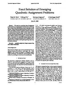
the expected return for asset i and σij is the covariance of returns for assets i and j. So, c is the vector of expected returns and Q is the n × n variance-covariance matrix of asset returns (Q is a symmetric positive semidefinite matrix which follows from the properties of variance-covariance matrices). Let x = (x1 , ..., xn )T denote the vector of asset holdings. In this case the expected return of the portfolio x is cT x and its variance is σ 2 = xT Qx. Markowitz [17] defined a portfolio to be efficient if for some fixed level of expected return no other portfolio gives smaller variance (risk). Equivalently, an efficient portfolio can be defined as the one for which at some fixed level of variance (risk) no other portfolio gives larger expected return. The determination of the efficient portfolio frontier in the Markowitz mean-variance model is equivalent to solving the following parametric QO problem due to Farrar [8] min −λcT x + 12 xT Qx s.t. Ax = b x ≥ 0.

(1.3.1)

Here, λ > 0 is an investor’s risk aversion parameter. The linear constraints Ax = b can represent budget constraints, bounds on asset holdings, etc. Nonnegativity constraints x ≥ 0 are short-sale constraints (non-negative asset holdings). If λ is allowed to vary, (1.3.1) becomes a parametric optimization problem. Furthermore, in this case solutions of the optimization problem for different values of λ trace the so-called efficient frontier in the mean-variance space. When λ is large, indicating high tolerance to risk, the solution of (1.3.1) is a portfolio with the highest expected return. When λ becomes smaller, the solution of the optimization problems will emphasize the minimization of the portfolio variance and put little weight on the maximization of the expected portfolio return. If we plot the solutions of a particular instance of problem (1.3.1) for different values of λ in the expected return – standard deviation coordinates, they 5



12

Expected Portfolio Return (percent per year)

11

λ=∞ 10

9

8

7

λ=0 6

5

4 3.5

Efficient Portfolio Frontier Corner Portfolios Individual Stocks 4

4.5

5

5.5

6

6.5

7

7.5

8

Standard Deviation (percent per year)

Figure 1.1: Mean-Variance Efficient Portfolio Frontier

trace the mean-variance efficient frontier (Figure 1.1). The mean-variance efficient frontier is known to be the graphical depiction of the Markowitz efficient set of portfolios and represents the boundary of the set of feasible portfolios that have the maximum return for a given level of risk. Portfolios above the frontier cannot be achieved. It was noticed that there exist some corner portfolios on the frontier, and in between this corner portfolios the frontier is piecewise quadratic. Figure 1.1 shows the efficient frontier in the mean-standard deviation space in order to be consistent with the existing literature. Note that, the efficient frontier is a piecewise quadratic function in the mean-variance space. From the observations it seems likely that we do not need to find a solution 6



of the parametric problem for every value of λ, but instead it is necessary to determine the corner portfolios only and ”restore” the efficient frontier between them by calculating the quadratic function.

1.4

Parametric Optimization: DSL Example

One of the recent examples of QO problems is a model of optimal multi-user spectrum management for Digital Subscriber Lines (DSL). Considering the behavior of this model under perturbations, we get a parametric quadratic problem. Moreover, the DSL model can have simultaneous perturbation of the coefficients in the objective function and in the right-hand side of the constraints. Let us consider a situation when M users are connected to one service provider via telephone line (DSL), where M cables are bundled together into the single one. The total bandwidth of the channel is divided into N subcarriers (frequency tones) that are shared by all users. Each user i tries to allocate his i total transmission power Pmax to subcarriers to maximize his data transfer rate N X

i pik = Pmax .

k=1

The bundling causes interference between the user lines at each subcarrier k = 1, . . . , N , that is represented by the matrix Ak of cross-talk coefficients. In addition, there is a background noise σk at frequency tone k. Current DSL systems use fixed power levels. In contrast, allocating each users’ total transmission power among the subcarriers ”intelligently” may result in higher overall achievable data rates. In noncooperative environment user i i allocates his total power Pmax selfishly across the frequency tones to maximize

his own rate. The DSL power allocation problem can be modelled as a multiuser noncooperative game. Nash equilibrium points of the noncooperative rate 7



maximization game correspond to optimal solutions of the following quadratic minimization problem: N X

N

1X T σk e pk + min pk Ak pk 2 k=1 k=1 N X i s.t. pik = Pmax , i = 1, . . . , M T

k=1

pk ≥ 0, k = 1, . . . , N,

T where pk = (p1k , . . . , pM k ) .

Engineers always look at the behavior of such models under different conditions. One of the parameters that influences the model is noisiness of the environment where the telephone cable is laid. The noisiness depends on the material the cable is made of, on the type of insulation used, etc. This noisiness, in turn, determines the background noise to the line σk . Users of telephone lines residing in noisy environments may get their total transmission power Pmax increased (i.e., get a more expensive modem) to improve the signal to noise ratio of the line. Such setup results in the parametric model: min

N X

N

(σk + λ△σk )eT pk +

k=1

s.t.

N X

1X T p Ak pk 2 k=1 k

i i + λ△Pmax , i = 1, . . . , M pik = Pmax

(1.4.1)

k=1

pk ≥ 0, k = 1, . . . , N

Parametric QO problem (1.4.1) represents a model with the noisiness parameter λ. The same parameter λ appears in the objective function and in the right-hand side of the constraints. The parametric model allows to look at the equilibria when the background noise and the total transmission power changes as λ varies. This formulation, for instance, can help answering such questions as: what happens if the background noise to the line increases two times faster than the total transmission power available to users. 8


1.5


Outline of the Thesis

The thesis describes the theoretical background of both quadratic optimization and parametric quadratic optimization as well as implementations of solution techniques for them into software packages. This predetermines the following organization of the thesis. In the current Chapter 1, we outline the history and the use of quadratic optimization techniques. In addition, we introduce the concept of parametric quadratic optimization and provide an example of portfolio problem which is formulated as parametric quadratic optimization problem. We also consider an engineering model that is formulated as simultaneous perturbation parametric optimization problem. Finally, the outline of the thesis is provided. Chapter 2 contains the background of using interior point methods for quadratic optimization. We use the homogenous embedding model and selfregular proximity functions. Chapter 2 also contains all theoretical results necessary for the implementation. Chapter 3 is devoted to the implementation of the interior point method algorithm outlined in Chapter 2. We describe the algorithm itself, problem specification formats, preprocessing and postprocessing, as well as the core of the methodology – sparse linear system solvers. Finally, we provide computational results to benchmark our software with existing quadratic solvers. In Chapter 4 we make a link from the quadratic optimization to its parametric counterpart. We provide the necessary background, prove some properties of such problems and suggest an algorithm for solving parametric quadratic optimization problems when the perturbation occurs simultaneously at the righthand side of the constraints and in the objective function. In addition, we specialize our results to parametric linear optimization. 9



Chapter 5 describes the implementation of the parametric programming algorithm in the MATLAB environment and provide an illustrative example of solving parametric problem. Chapter 5 also presents our computational results. Finally, Chapter 6 contains concluding remarks and suggestions for future work.

10

Chapter 2 Interior Point Methods for Quadratic Optimization Problems In this chapter we extend our introductory knowledge about quadratic optimization (QO) problems, describe their properties and solution techniques. As we already know, QO problem consists of minimizing a convex quadratic objective function subject to linear constraints. In addition to showing problem formulations, we review the duality theory for QO problems. Finally, Interior Point Methods (IPMs) for solving these problems are described. Results presented in this chapter are mainly based on [2], [35] and [36].

2.1

Quadratic Optimization Problems

A primal convex QO problem is defined as: (QP )

min cT x + 21 xT Qx s.t. Ax = b x ≥ 0,

(2.1.1)

where Q ∈ IRn×n is a symmetric positive semidefinite matrix, A ∈ IRm×n , rank(A) = m, c ∈ IRn , b ∈ IRm are fixed data and x ∈ IRn is an unknown 11



vector. The Wolfe Dual of (QP ) is given by (QD)

max bT y − 21 uT Qu s.t. AT y + z − Qu = c z ≥ 0,

(2.1.2)

where z, u ∈ IRn and y ∈ IRm are unknown vectors. Note that when Q = 0 we get a Linear Optimization (LO) problem. The feasible regions of (QP ) and (QD) are denoted by QP = {x : Ax = b, x ≥ 0}, QD = {(u, y, z) : AT y + z − Qu = c, z, u ≥ 0}, and their associated optimal solution sets are QP ∗ and QD∗ , respectively. It is known that for any optimal solution of (QP ) and (QD) we have Qx = Qu and xT z = 0, see e.g., Dorn [7]. It is also known from [7] that there are optimal solutions with x = u. Since we are only interested in the solutions where x = u, therefore, u will be replaced by x in the dual problem. The duality gap cT x + xT Qx − bT y = xT z being zero is equivalent to xi zi = 0 for all i ∈ {1, 2, . . . , n}. This property of the nonnegative variables x and z is called the complementarity property. Solving primal problem (QP ) or dual problem (QD) is equivalent to solving the following system, which represents the Karush-Kuhn-Tucker (KKT) optimality conditions [33]: Ax − b = 0, x ≥ 0, AT y + z − Qx − c = 0, z ≥ 0, xT z = 0,

(2.1.3)

where the first line is the primal feasibility, the second line is the dual feasibility, and the last line is the complementarity condition. The complementarity condi12



tion can be rewritten as xz = 0, where xz denotes the componentwise product of the vectors x and z. System (2.1.3) is referred to as the optimality conditions. Let X = diag(x1 , . . . , xn ) and Z = diag(z1 , . . . , zn ) be the diagonal matrices with vectors x and z forming the diagonals, respectively. For LO the GoldmanTucker Theorem states that there exists a strictly complementary optimal solution (x, y, z) if both the primal and dual problems are feasible. For LO, the feasible primal-dual pair (x, y, z) is strictly complementary if xi zi = 0 and xi + zi > 0 for all i = 1, . . . , n. Equivalently, strict complementarity can be characterized by xz = 0 and rank(X) + rank(Z) = n. Unlike in LO, where strictly complementary optimal solution always exists, for QO the existence of such solution is not ensured. Instead, a maximally complementary solution can be found. A pair of optimal solutions (x, y, z) for the QO problem is maximally complementary if it maximizes rank(X) + rank(Z) over all optimal solution pairs. As we see in Chapter 4, this leads to tri-partition of the optimal solution set.

2.2

Primal-Dual IPMs for QO

Primal-dual IPMs are iterative algorithms that aim to find a solution satisfying the optimality conditions (2.1.3). IPMs generate a sequence of iterates (xk , y k , z k ), k = 0, 1, 2, . . . that satisfy the strict positivity (interior point) condition xk > 0 and z k > 0, but feasibility (for infeasible IPMs) and optimality are reached as k goes to infinity. In this thesis we are concerned about feasible IPM methods which produce a sequence of iterates where the following interior point condition (IPC) holds for every iterate (x, y, z) Ax = b, x > 0, A y + z − Qx = c, z > 0. T

13

(2.2.1)


2.2.1


The Central Path

We perturb the complementarity condition in the optimality conditions (2.1.3) as

Ax = b, x > 0, A y + z − Qx = c, z > 0, Xz = µe, T

(2.2.2)

where µ > 0 and e = (1, . . . , 1)T . It is obvious that the last nonlinear equation in (2.2.2) becomes the complementarity condition for µ = 0. A desired property of system (2.2.2) is the uniqueness of its solution for each µ > 0. The following theorem [12] shows such conditions. Theorem 2.2.1 System (2.2.2) has a unique solution for each µ > 0 if and only if rank(A) = m and the IPC holds for some point. When µ is running through all positive numbers, the set of unique solutions (x(µ), y(µ), z(µ)) of (2.2.2) define the so-called primal-dual central path. The sets {x(µ) | µ > 0} and {(y(µ), z(µ)) | µ > 0} are called primal central path and dual central path respectively. One iteration of primal-dual IPMs consists of taking a Newton step applied to the central path equations (2.2.2) for a given µ. The central path stays in the interior of the feasible region and the algorithm approximately follows it towards optimality. For µ → 0 the set of points (x(µ), y(µ), z(µ)) gives us a maximally complementary optimal solution of (QP) and (QD).

2.2.2

Computing the Newton Step

Newton’s method is used to solve the system (2.2.2) iteratively. At each step we need to compute the direction (△x, △y, △z). A new point in the computed

14



direction (x + △x, y + △y, z + △z) should satisfy A(x + △x) = b, A (y + △y) + (z + △z) − Q(x + △x) = c, (x + △x)(z + △z) = µe. T

For a given strictly feasible primal-dual pair (x, y, z) we can write this system with the variables (△x, △y, △z) as A△x = 0, AT △y + △z − Q△x = 0, x△z + z△x + △x△z = µe − xz.

(2.2.3)

System (2.2.3) is non-linear. Consequently, the Newton step is obtained by dropping the non-linear term that gives the linearized Newton system A△x = 0, A △y + △z − Q△x = 0, x△z + z△x = µe − xz. T

(2.2.4)

The linear system (2.2.4) is referred to as the primal-dual Newton system. It has 2n + m equations and 2n + m unknowns. The system has a unique solution if rank(A) = m. In matrix form the Newton system (2.2.4) can be written as      0 A 0 0 △x .  −Q AT I   △y  =  0 µe − Xz Z 0 X △z

(2.2.5)

Solving system (2.2.5) for △z gives

△z = X −1 (µe − Xz − Z△x), and substituting △z into system (2.2.5) we get ¶µ ¶ µ ¶ µ △x µX −1 e − z −Q − D AT = , A 0 △y 0 where D = X −1 Z is a diagonal matrix with Dii = (2.2.6) is called the augmented system. 15

zi xi

(2.2.6)

for i = 1, . . . , n. System



From the first equation of (2.2.6) we can express △x as △x = (Q + D)−1 (AT △y − µX −1 e + z). Then the augmented system reduces to: A(Q + D)−1 AT △y = A(Q + D)−1 (µX −1 e − z),

(2.2.7)

that is often called the normal equation form.

2.2.3

Step Length

In this section we describe how to determine the next iteration point. After solving the Newton system (2.2.5) we are getting the search direction (∆x, ∆y, ∆z). This Newton search direction is computed assuming that the step length α is equal to one. But taking such step can lead to loosing strict feasibility of the solution as (x+∆x, y +∆y, z +∆z) might be infeasible. Our goal is to keep strict feasibility, therefore we want to find such an α that the next iteration point is strictly feasible, i.e., (xk+1 , yk+1 , zk+1 ) = (xk , yk , zk ) + α(∆xk , ∆yk , ∆zk ), with xk+1 > 0 and zk+1 > 0. This can be done in two steps: • find the maximum possible step size αmax such that ½µ ¶ µ ¶ ¾ x △x max α = arg max +α ≥0 , z △z α>0 • as strict feasibility is not warranted by the previous step, we need to use a damping factor ρ ∈ (0, 1) to choose such α that α = min{ραmax , 1}. 16



Finally, we can compute αmax in the following way: −xj , j = 1, . . . , n}, ∆xj 0; an accuracy parameter ǫ > 0; an update parameter 0 < θ < 1; µ0 = 1, k = 0; (x0 , y 0 , z 0 ) satisfying x0 > 0, z 0 > 0 and Ψ(x0 z 0 , µ0 ) ≤ δ;

begin

while (xk )T z k ≥ ǫ do begin

µk = (1 − θ)( (x

k )T z k

n k

);

while Ψ(xk z k , µ ) ≥ δ

do

begin

solve the Newton system (2.2.5) to find (△xk , △y k , △z k );

determine the step size α;

xk = xk + α△xk , y k = y k + α△y k , z k = z k + α△z k ; end xk+1 = xk , y k+1 = y k , z k+1 = z k , k = k + 1; end end

2.3

Homogeneous Embedding Model

In this section we present a homogeneous algorithm to solve the QO problem. The homogeneous embedding model is one of the ways to formulate the system of linear equations associated with the QO problem. Such model for the LO has been developed by Ye, Todd and Mizuno [32]. Later on it was extended by

18



Anderson and Ye [2] to monotone complementarity problems (MCP). The QO problem is a special case of MCP and so, the algorithm applies for QO as well.

2.3.1

Description of the Homogeneous Embedding Model

From the Weak Duality Theorem it follows that system (2.1.3) is equivalent to Ax − b = 0, x ≥ 0, AT y + z − Qx − c = 0, s ≥ 0, bT y − cT x − xT Qx ≥ 0.

(2.3.1)

A way to solve system (2.3.1) is to introduce a slack variable κ for the last inequality in the system and a homogenization variable τ . The following system is a homogeneous reformulation of the QO problem: Ax − bτ = 0, x ≥ 0, τ ≥ 0, AT y + z − Qx − cτ = 0, z ≥ 0, y free, T bT y − cT x − x τQx − κ = 0, κ ≥ 0.

(2.3.2)

System (2.3.2) has some attractive properties. First, with τ = 1 and κ = 0 the solution of the system (2.3.2) gives an optimal solution of the QO problem. Second, it has zero as its trivial solution and can be considered as an MCP with zero right-hand side vector. Third, considered as an MCP, system (2.3.2) does not satisfy the IPC. The modification of problem (2.3.2) to a homogeneous problem having an interior point is (Anderson and Ye [2]) min xT z + τ κ s.t. Ax T −A y + Qx bT y − c T x T rPT y + rD x y, ν free, x ≥ 0,

− bτ + cτ T − x τQx + rG τ τ ≥ 0, z

− rP ν = 0, − rD ν − z = 0, − rG ν − κ = 0, = −β, ≥ 0, κ ≥ 0,

(2.3.3)

where ν is an artificial variable added in order to satisfy the IPC, the coefficients rP , rD and rG represent the infeasibility of the primal and dual initial interior 19



points and the duality gap, respectively. These coefficients for a given initial point (x0 > 0, y 0 , z 0 > 0, τ 0 > 0, κ0 > 0, ν 0 > 0) are defined as follows: rP = (Ax0 − bτ 0 )/ν0 , rD = (−AT y 0 + Qx0 + cτ 0 − z 0 )/ν0 , 0T

0

rG = (bT y 0 − cT x0 − x τQx − κ0 )/ν0 , 0 T 0 β = −rPT y 0 − rD x − rG τ 0 .

The homogeneous embedding model (2.3.3) has several advantages. First, the algorithm based on it does not need to use a ”big-M” penalty parameter [2]. Second, by utilizing the homogeneous embedding model we can avoid using the two-phase method, where we need to find a feasible interior initial point to start with, that even might not exist for many problems. It is not difficult to note that for properly chosen rP , rD and rG the point (x0 = e, y 0 = 0, z 0 = e, τ 0 = 1, κ0 = 1, ν 0 = 1) is feasible for the embedding model. Third, the homogeneous embedding model generates a solution sequence converging towards an optimal solution of the original problem, or it produces an infeasibility certificate for either (QP ), or (QD), or for both. We can apply the IPM algorithm outlined in Section 2.2.4 for solving the homogeneous embedding model. The size of the Newton system for this model is not significantly larger than the size of the original system. Finally, a small update IPM for solving the homogeneous model √ has the iteration bound O( n log nǫ ).

2.3.2

Finding Optimal Solution

Let us consider a strictly complementary solution (y ∗ , x∗ , τ ∗ , ν ∗ = 0, z ∗ , κ∗ ) of the homogeneous problem (2.3.3). Our goal is to recover the information about solutions of the original primal (QP ) and dual (QD) QO problems. We distinguish three cases: ∗

1. If τ ∗ > 0 and κ∗ = 0, then ( xτ ∗ , τz ∗ , τy ∗ ) is a strictly complementary optimal ∗

∗

20



solution for (QP ) and (QD). 2. If τ ∗ = 0 and κ∗ > 0, the solution of the embedding model provides a Farkas certificate for the infeasibility of the dual and/or primal problems and then: • if cT x∗ < 0, then the dual problem (QD) is infeasible; • if −bT y ∗ < 0, then the primal problem (QP ) is infeasible; • if cT x∗ < 0 and −bT y ∗ < 0, then both primal (QP ) and dual (QD) problems are infeasible. 3. If τ ∗ = 0 and κ∗ = 0 then neither a finite solution nor a certificate proving infeasibility exists. This cannot happen for convex QO problems, because if no optimal solutions exist, then an infeasibility certificate always exist [33]. Let us prove the conclusion of case 2. For τ ∗ = 0, κ∗ > 0 and ν ∗ = 0 we have Ax∗ = 0, A y − Qx + z ∗ = 0. T ∗

∗

In addition, the third constraint of (2.3.3) imply that bT y ∗ − c T x∗ − and as κ∗ > 0 and

x∗T Qx∗ τ∗

x∗ T Qx∗ − κ∗ = 0, τ∗

≥ 0, thus bT y ∗ − cT x∗ > 0,

i.e., cT x∗ − bT y ∗ < 0. 21



The last inequality means that at least one of the components of the left-hand side, namely cT x∗ or −bT y ∗ , is strictly less than zero. Let us consider these three cases separately: • Consider the case when cT x∗ < 0. Let us assume to the contrary that a feasible solution (x∗ , yˆ, zˆ) for the dual problem such that zˆ ≥ 0 and AT yˆ − Qx∗ + zˆ = c exists. Then 0 > = = = ≥

cT x ∗ (AT yˆ − Qx∗ + zˆ)T x∗ yˆT (Ax∗ ) − x∗ T Qx∗ + zˆT x∗ zˆT x∗ 0,

that is a contradiction. Consequently, the dual problem is infeasible. • Consider the case when −bT y ∗ < 0. Let us assume to the contrary that a feasible solution xˆ for the primal problem such that xˆ ≥ 0 and Aˆ x=b exists. Then

0 > = = = ≥

−bT y ∗ (−Aˆ x)T y ∗ T xˆ (−AT y ∗ ) xˆT z ∗ 0,

that is a contradiction. Consequently, the primal problem is infeasible. • If both cT x∗ < 0 and −bT y ∗ < 0, then by the same reasoning we get both the primal and dual problems to be infeasible.

2.4

Computational Practice

The majority of QO problems are not given in the standard form (2.1.1). Instead, problem formulations may include inequality constraints, free variables as well as lower and upper bounds on the variables. In this section we derive the augmented 22



system of the type (2.2.6) and the normal equations of the type (2.2.7) for such formulations using the homogeneous embedding model. The first step in this process is the preprocessing stage when problem transformations are applied to bring a general form problem to the standard form (2.1.1), while upper bounds for the variables are allowed and treated separately. These transformations are referred to as preprocessing. If a QO problem has inequality constraints A˜ x ≤ b and non-negativity constraints x˜ ≥ 0, non-negative slack variables x¯ are added to the constraints to transform the problem to the standard form µ ¶ µ ¶ x˜ x˜ (A I) = b, ≥ 0, x¯ x¯ where I is the identity matrix of appropriate dimension. If a problem contains variables xj not restricted to be non-negative (free variables), then these variables are split to two non-negative variables xj = x+ j −

+ − x− j , xj ≥ 0, xj ≥ 0. So, after taking care of inequality constraints and free

variables we get a larger problem conform with the standard form (2.1.1). Problems including variables that have upper and lower bounds require more attention. If a variable has a lower bound xi ≥ li , then we shift the lower bound to zero by substituting the variable xi by xi − li ≥ 0. Appropriate changes should be made in the vectors c and b: c is substituted by c + Q l and b by b − A l. If the variable had an upper bound xi ≤ ui , then this upper bound is shifted as well ui = ui − li . After such shift we have a problem of the same size with nonnegative variables and possible upper bounds on some variables. The appropriate back transformation of variables should be made after solving the QO problems at the postprocessing stage. For the variables having upper bounds xi ≤ ui , extra slack variables are added to transform the inequality constraints to equality constraints. This ob23



viously leads to increase in the number of variables and constraints. So, the last two sets of constraints of the primal QO problem min cT x + 12 xT Qx s.t. Ax = b, 0 ≤ xi ≤ ui , i ∈ I, 0 ≤ xj , j ∈ J,

(2.4.1)

where A ∈ IRm×n , c, x ∈ IRn , b ∈ IRm , and I and J are disjoint partition of the index set {1, . . . , n}, can be rewritten as F x + s = u, x ≥ 0, s ≥ 0, F ∈ IRmf ×n , where mf = |I| and s ∈ IRmf is the slack vector. Matrix F consists of the unit vectors associated with the index set I as its rows. Consequently, the QO problem becomes

Its dual is

min cT x + 21 xT Qx s.t. Ax = b Fx + s = u x ≥ 0, s ≥ 0.

(2.4.2)

min bT y − uT w − 21 xT Qx s.t. AT y − F T w + z − Qx = c, w ≥ 0, z ≥ 0.

(2.4.3)

where y ∈ IRm , w ∈ IRmf and z ∈ IRn . The complementarity gap is gap = cT x + 12 xT Qx − (bT y − uT w − 21 xT Qx) = (AT y − F T w + z − Qx)T x − y T (Ax) + wT (F x + s) + xT Qx = xT z + sT w. Finally, the optimality conditions for (2.4.2) and (2.4.3) can be written as Ax Fx + s AT y − F T w + z − Qx Xz Sw 24

= = = = =

b, u, c, 0, 0.

(2.4.4)


2.4.1


Solving Homogeneous Embedding Model with Upper Bound Constrains

Addition of the primal equality constraint F x+s = u to the problem formulation results in the following homogeneous embedding model that is a straightforward generalization of (2.3.3): min xT z + sT w + τ κ s.t. Ax − bτ − rP 1 ν = 0, − F x + uτ − rP 2 ν − s = 0, T T −A y + F w + Qx + cτ − rD ν −z = 0, xT Qx T T T b y − u w − c x − τ − rG ν − κ = 0, T rPT 1 y + rPT 2 w + rD x + rG τ = −β, y, ν free, w ≥ 0, x ≥ 0, τ ≥ 0, z ≥ 0, s ≥ 0, κ ≥ 0, where

(2.4.5)

rP 1 = (Ax0 − bτ 0 )/ν0 , rP 2 = (−F x0 + uτ 0 − s0 )/ν0 , rD = (−AT y 0 + F T w0 + Qx0 + cτ 0 − z 0 )/ν0 , 0T

0

− κ0 )/ν0 , rG = (bT y 0 − uT w0 − cT x0 − x τQx 0 T 0 β = −rPT 1 y 0 − rPT 2 w0 − rD x − rG τ 0 .

The objective function of problem (2.4.5) can be also expressed as follows. Multiplying the first, second, third, forth and fifth equality constraints of (2.4.5) by y T , wT , xT , τ and ν correspondingly, and summing them up, we get xT z + sT w + τ κ = νβ. Designing the IPM algorithm for the homogeneous embedding model we can follow the same reasoning as in Section 2.2.1 and define the central path for problem (2.4.5). The central path is the set of solutions of the following system

25



for all µ > 0: − T T −A y + F w + b T y − uT w − rPT 1 y + rPT 2 w +

Ax Fx Qx cT x T rD x

− bτ + uτ + cτ T − x τQx + rG τ

The Newton system for (2.4.6) is  0 0 A −b  0 0 −F u  T −A F T Q c   bT −uT −cT − 2xT Q xT Qx  τ τ2 T T T  rT r r r P2 D G  P1  0 S 0 0   0 0 Z 0 0 0 0 κ

where

− − − −

rP 1 ν rP 2 ν − s rD ν −z rG ν − κ

= 0, = 0, = 0, = 0, = −β, Xz = µe, Sw = µe, τκ = µ.

(2.4.6)

    −rP 1 0 0 0 0 △y △w  0  −rP 2 −I 0 0          −rD 0 −I 0  △x  0      −rG 0 0 −1 △τ = 0  , (2.4.7)     0 0 0 0  △ν   0      0 W 0 0 △s rsw 0 0 X 0 △z  rxz rτ κ △κ 0 0 0 τ

rsw = µe − Sw, rxz = µe − Xz, rτ κ = µe − τ κ.

From the last three lines of (2.4.7) we get

△s = W −1 (rsw − S△w), △z = X −1 (rxz − Z△x), △κ = τ −1 (rτ κ − κ△τ ).

(2.4.8)

We also have △ν =

T T rsw e + rxz e + rτ κ . β

Consequently, system (2.4.7) reduces to  0 0 A −b −1  0 W S −F u  T T −1  −A F Q+X Z c xT Qx 2xT Q T T T + b −u −c − τ τ2 26

  ′ r △y ′   △w   rsw = ′    △x   rxz △τ rτ′ κ 

κ τ



 , 

(2.4.9)

M.Sc. Thesis - Oleksandr Romanko where

r′ = ′ rsw = ′ rxz = rτ′ κ =


rP 1 △ν, rP 2 △ν + W −1 rsw , rD △ν + X −1 rxz , rG △ν + τ −1 rτ κ .

From the second equation of (2.4.9) we get

′ △w = W S −1 rsw + W S −1 F △x − W S −1 u△τ,

(2.4.10)

that allows us to reduce the system to     ′′  Q+X −1 Z +F T W S −1 F −AT c − F T W S −1 u rxz △y      A 0 −b △x = r′′ , (2.4.11) TQ T Qx 2x x rτ′′κ −cT − τ −uT W S −1 F bT + κτ +uT W S −1 u △τ τ2 where

D−1 r′′ ′′ rxz rτ′′κ

= = = =

Q + X −1 Z + F T W S −1 F, r′ , ′ ′ rxz − F T W S −1 rsw , ′ T −1 ′ rτ κ + u W S rsw .

Equation (2.4.11) is the augmented system. From the second equation of (2.4.11), we have ′′ △x = Drxz + DAT △y − D(c − F T W S −1 u)△τ.

Consequently, system (2.4.11) reduces to ¶µ ¶ µ ′′′ ¶ µ △y r ADAT a1 , = 2 T 3 rτ′′′κ △τ −(a ) a

(2.4.12)

where a1 −(a2 )T a3 r′′′ rτ′′′κ

= −b − AD(c − F T W S −1 u), T = bT − (cT + 2xτ Q + uT W S −1 F )DAT , T T = x τQx + κτ + uT W S −1 u + (cT + 2xτ Q + uT W S −1 F )D(c − F T W S −1 u), 2 ′′ = r′′ − ADrxz , T ′′ T ′′ = rτ κ + (c + 2xτ Q + uT W S −1 F )Drxz .

From the last equation of (2.4.12), we get △τ =

1 ′′′ (r + (a2 )T △y), a3 τ κ 27



and then system (2.4.12) reduces even further to aT ]△y = ξ, [ADAT + aˆ where a =

a1 , a3

a ˆ = a2 and ξ = r′′′ −

(2.4.13)

rτ′′′κ 1 a. a3

At this point we have two choices: to solve the normal equations (2.4.13) or to solve the augmented system (2.4.11). First, let us reduce the augmented system (2.4.11) by rewriting it in the  −Q − X −1 Z − F T W S −1 F AT  A 0 ′′ T −(a ) bT

where

following form:     ′′ −rxz △y −a′ −b   △x  =  r′′  , (2.4.14) rτ′′κ △τ a′′′

a′ = c − F T W S −1 u, a′′ = c + 2Qx + F T W S −1 u, τ T + κτ + uT W S −1 u. a′′′ = x τQx 2

From the last equation of (2.4.14), we get: " µ ¶# ¶T µ 1 −a′′ △y ′′ , △τ = ′′′ rτ κ − △x b a

(2.4.15)

and then system (2.4.14) reduces to: ! ¶ ·µ ¸ µ ¶ Ã ′′ ′′ −Q − X −1 Z − F T W S −1 F AT △y −rxz + a′ raτ′′′κ T +a ã ˇ = , (2.4.16) ′′ A 0 △x r′′ + b raτ′′′κ where a ˜ =

µ

T

1 a′′′

a ˇ

=

a′ b µ

¶

,

−a′′ b

¶T

.

Now, we have got two linear systems: the normal equations and the augmented system. We can solve either of them to find the solution of the Newton system for the homogeneous model and get the search direction for IPMs QO algorithms. Efficient solution of those systems is the subject of Section 2.5. 28


2.4.2


Step Length

We can follow the same reasoning as in Section 2.2.3 to derive analogous results about the step length for the homogeneous embedding model. After solving the augmented system (2.4.16), we obtain ∆y and ∆x. Doing back substitutions to the equations (2.4.15), (2.4.10) and (2.4.8) we get ∆τ , ∆w, ∆z, ∆s and ∆κ. The maximum acceptable step length α for getting strictly interior point in the next iteration is determined as follows: αxmax = αzmax = max αw =

αsmax = ατmax = κ αmax = α =

−xj , j = 1, . . . , n}, ∆xj κk tol kt the problem is non-firm infeasible and we move to the next iteration k + 1. If the solution is still 51



non-firm infeasible after a couple of iterations as for numerical reasons no more precise solution can be reached, infeasibility is reported up to a certain precision.

3.5

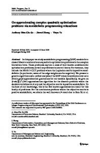
Numerical Results

In this section our computational results for the McIPM-QO solver are presented. All computations are performed on an IBM RS/6000 workstation with four processors and 8Gb RAM. The operating system is IBM AIX 4.3. The test problems used for our numerical testing are coming from the Maros and Mészáros QP test set [18] which consist of 138 problems. The sizes of problems vary from a couple of variables to around 300, 000 variables. You can find the description of the problems in the testset, including original problem dimensions and problem dimensions after McIPM preprocessing, in Appendix B. The McIPM parameter settings used for testing are the following: % PARAMETERS - Algorithmic parameters for MCIPM p

= 1;

q

= 1;

regeps

= 1.e-9;

% regularization

MAXITER

= 150;

% Maximum number of iteration

tol emb

= 5.0e-17;

% an accuracy parameter for mu

tol ori

= 5.0e-09;

% an accuracy parameter for gap ori

tol end

= 1.e-15;

% an accuracy parameter for nu

tol bad

= 1.e-15;

tol kt

= 1.e-3;

% an accuracy parameter for tau/ka

damp

= 0.995;

% a variable damping parameter

bad step

= 0.4;

worst step= 0.1; MAXQ

= 3; The testing results are shown in Tables 3.1, 3.2 and 3.3. As there are no 52



standard confirmed solutions for the test set, we have solved all the problems with CPLEX and MOSEK and also used the BPMPD solution reported in [22] for comparison. In columns ’Diff.’ of Tables 3.1–3.3 we report the difference of the optimal solutions found by McIPM with the solutions found by CPLEX, MOSEK and BPMPD (ObjCP LEX − ObjM cIP M , ObjM OSEK − ObjM cIP M and

ObjBP M P D − ObjM cIP M ). Furthermore, column ’Sign. digits’ shows

the number of significant digits in the McIPM solutions as compared with the solutions found by CPLEX, MOSEK and BPMPD. We also report the number of iterations ’Iter’, optimal function value ’Objective’ and CPU time. Column ’Resid.’ is McIPM error computed according to (3.4.6). All the test were done using the LDL package for solving the augmented system. As we see from the results, McIPM produces reliable solutions with six or more significant digits for the majority of the problems. The problematic problems are depicted in bold font. The imprecise solution on this set of problems is due to precision of solving the Newton system with the default regularization parameter 10−9 . The two sparse linear packages – LDL and McSML – are not always able to produce precise solutions due to numerical difficulties, that result in less precise solutions produced by McIPM. We plan to use iterative refinement of solution of the liner system produced by LDL to improve the current results. It is worth mentioning that using different regularization, solving the linear system without ordering and regularization with the LDL package (it works in most cases as zero elements does not appear in the diagonal in the upper left block E of the matrix) or employing McSML as sparse linear system solver allow to get the solution precision of seven or more significant digits for all the problems in the test set except for the largest problem boyd2 which has

four significant digits in the solution. Table 3.4 shows the solutions to boldfont problematic problems in Tables 3.1–3.3 computed using McSML or LDL without ordering and regularization of the augmented system. In general, almost all packages experience troubles on the number of problems shown in Table 3.4. One can notice that McIPM has lower number of iterations than CPLEX or

53



MOSEK on the majority of difficult problems. Solution precision on this set of difficult problems is not very good especially for commercial solvers, furthermore, MOSEK and BPMPD produce incorrect solutions for one problem each. Comparison of the number of iterations used by CPLEX, MOSEK and McIPM does not show a clear trend, but in the majority of the cases McIPM beats the commercial packages confirming that the usage of self-regular proximity functions and search directions can reduce the number of IPM iterations. In the column ’#iter q>1’ we show the number of iterations when self-regular parameter q was dynamically increased from 1 to 3. The solution time of McIPM in most cases is more than the one of CPLEX and MOSEK. This is partially explained by the fact that CPLEX and MOSEK are pure C packages while McIPM is partially coded in Matlab. The second reason for the difference in solution time is that all packages – CPLEX, MOSEK and BPMPD are utilizing more advanced preprocessing techniques than McIPM. For example, BPMPD reduces problem size for the problem qcapri from 271 × 373 to 148 × 214 while

McIPM only to 267 × 353. Similarly, MOSEK reduces the size of the largest

problem in the test set boyd2 from 186531 × 279785 to 119721 × 150580 while

McIPM leaves it unchanged.

We do not show all the results obtained when the McSML package is employed for solving the augmented systems as it generally exhibit slightly poorer performance than LDL. Still, McIPM with the McSML sparse linear solver is able to solve more than 90% of the test set problems. In general, we may conclude that McIPM is competitive even with the commercial packages. One of the sources for improving competitiveness is the possibility of using more advanced sparse linear algebra packages, e.g., TAUCS, which does not have separate symbolic and numeric LDLT factorization at the moment but plans to have it in the future. Another possibility is to get McSML to the state of the art by implementing Bunch-Parlett or Bunch-Kaufman techniques. The other option is porting McIPM to C language for improving its speed.

54

55

1 1 17 20 1 1 13 16 40 53 12 14 12 13 12 16 19 11 11 12 9 11 13 10 12 5 1 16 14 17 14 16 15 12 13

aug2d aug2dc aug2dcqp aug2dqp aug3d aug3dc aug3dcqp aug3dqp boyd1 boyd2 cont-050 cont-100 cont-101 cont-200 cont-201 cont-300 cvxqp1_l cvxqp1_m cvxqp1_s cvxqp2_l cvxqp2_m cvxqp2_s cvxqp3_l cvxqp3_m cvxqp3_s dpklo1 dtoc3 dual1 dual2 dual3 dual4 dualc1 dualc2 dualc5 dualc8 exdata genhs28 gouldqp2 gouldqp3 hs118 hs21 hs268 hs35 hs35mod hs51 hs52

4 20 11 14 22 18 22 26 10 3

Iter

Name

Prob.

5 5 13 15 4 4 11 12 27 40 11 12 12 12 12 13 11 10 8 11 10 9 10 11 10 4 5 13 12 13 12 18 15 9 15 15 4 15 8 10 10 14 5 10 4 3

CPU sec. Iter

1.6874117529E+06 0.51 1.8183680656E+06 0.49 6.4981347395E+06 3.27 3.83 6.2370120256E+06 0.03 5.5406772579E+02 0.07 7.7126243870E+02 9.9336214653E+02 0.29 6.7523767128E+02 0.31 28.91 -6.1735219641E+07 89.67 2.1256767267E+01 -4.5638509043E+00 0.62 6.66 -4.6443978688E+00 5.54 1.9552732466E-01 -4.6848759204E+00 47.18 46.07 1.9248337744E-01 1.9151234551E-01 157.68 1.0870479970E+08 2911.07 8.70 1.0875115683E+06 1.1590718119E+04 0.04 8.1842458279E+07 608.78 8.2015543102E+05 3.44 8.1209404773E+03 0.02 1.1571110487E+08 2998.47 1.3628286862E+06 15.51 1.1943432202E+04 0.05 3.7009621711E-01 0.01 2.3526248053E+02 0.30 3.5012965733E-02 0.06 0.06 3.3733676123E-02 0.11 1.3575583687E-01 7.4609084180E-01 0.04 6.1552508295E+03 0.00 3.5513076927E+03 0.00 4.2723232678E+02 0.00 1.8309358833E+04 0.00 MPS read error 9.2717369377E-01 0.00 1.8427450336E-04 0.08 2.0627840000E+00 0.07 6.6482045000E+02 0.00 -9.9960000000E+01 0.01 0.0000000000E+00 0.00 1.1111111110E-01 0.00 2.5000000000E-01 0.00 0.0000000000E+00 0.00 5.3266475645E+00 0.00

Objective

CPLEX CPU sec.

Objective

BPMPD Iter

Resid.

Objective

McIPM CPU se c.

#iter q>1

Differ.

12 10 8 10 8 9 8 9 14 11

10 10 10 10 10 11 10 10 11 1 11 11 11 11 9 8 6 10 11 10 11 11 9 8 9 12 9 11 11 10 11 10 11 11 11

Sign. digits

Comp. CPLEX

8 6.45E-10 1.6874117518E+06 1 5.30 0 1.10E-03 1.6874117523E+06 4.10 1.6874118E+06 1.8183680651E+06 3.90 1.8183681E+06 8 7.24E-10 1.8183680651E+06 14.54 0 5.00E-04 16 7.42E-10 6.4981347403E+06 14.86 3 -8.00E-04 6.4981347406E+06 5.00 6.4981348E+06 6.2370120296E+06 5.40 6.2370121E+06 17 1.80E-09 6.2370120309E+06 14.78 4 -5.30E-03 0.99 5.5406773E+02 6 4.28E-10 5.5406772570E+02 1.66 0 9.00E-08 5.5406772537E+02 6 3.67E-10 7.7126243864E+02 1.71 0 6.00E-08 1.00 7.7126244E+02 7.7126243826E+02 9.9336214683E+02 0.95 9.9336215E+02 10 4.25E-09 9.9336214592E+02 1.40 0 6.10E-07 6.7523767233E+02 0.97 6.7523767E+02 12 1.59E-09 6.7523767156E+02 1.59 0 -2.80E-07 -6.1735219617E+07 13.42 -6.1735220E+07 24 2.61E-09 -6.1735219641E+07 107.12 2 0.00E+00 2.1256766951E+01 65.93 2.1256767E+01 150 8.96E-05 2.8212092551E+01 2259.17 134 -6.96E+00 -4.5638509043E+00 3.49 1 -4.00E-10 1.70 -4.5638509E+00 11 1.50E-09 -4.5638509039E+00 12 5.47E-10 -4.6443978687E+00 19.28 0 -1.00E-10 -4.6443978688E+00 11.00 -4.6443979E+00 1.9552732466E-01 9.10 1.9552733E-01 13 1.86E-09 1.9552732468E-01 20.85 2 -2.00E-11 -4.6848759204E+00 80.00 -4.6848759E+00 12 2.78E-09 -4.6848759203E+00 138.84 0 -1.00E-10 1.9248337287E-01 74.00 1.9248337E-01 12 4.91E-09 1.9248337305E-01 144.25 1 4.39E-09 1.9151228591E-01 270.00 1.9151232E-01 16 4.08E-10 1.9151228607E-01 730.20 3 5.94E-08 1.0870480011E+08 1600.00 1.0870480E+08 59 3.32E-05 1.0870457545E+08 2498.81 12 2.24E+02 1.0875115706E+06 2.90 1.0875116E+06 11 1.51E-09 1.0875115682E+06 2.06 0 1.00E-04 1.1590718121E+04 0.62 1.1590718E+04 9 5.88E-11 1.1590718120E+04 0.26 0 -1.00E-06 8.1842458398E+07 240.00 8.1842458E+07 12 1.91E-09 8.1842458309E+07 446.92 0 -3.00E-02 8.2015543142E+05 11 2.24E-10 8.2015543106E+05 1.57 0 -4.00E-05 1.30 8.2015543E+05 8.1209404992E+03 0.62 8.1209405E+03 9 1.77E-09 8.1209404779E+03 0.26 0 -6.00E-07 1.1571112450E+08 4800.00 1.1571110E+08 16 1.27E-06 1.1571110447E+08 739.13 0 4.00E-01 1.3628287420E+06 7.60 1.3628287E+06 14 3.17E-10 1.3628287416E+06 2.75 0 -5.54E-02 1.1943432203E+04 0.64 1.1943432E+04 9 1.34E-09 1.1943432222E+04 0.25 0 -2.00E-05 3.7009621681E-01 0.63 3.7009622E-01 6 3.69E-11 3.7009621711E-01 0.18 0 0.00E+00 2.3526248103E+02 3.10 2.3526248E+02 7 4.48E-11 2.3526248105E+02 6.45 0 -5.20E-07 3.5012969824E-02 0.63 3.5012966E-02 14 4.99E-10 3.5012965875E-02 0.49 0 -1.42E-10 0.47 0 -5.50E-11 3.3733676124E-02 0.65 3.3733676E-02 12 2.42E-09 3.3733676178E-02 1.3575583742E-01 0.68 1.3575584E-01 13 8.11E-10 1.3575583716E-01 0.61 0 -2.90E-10 7.4609084264E-01 0.66 7.4609084E-01 12 3.34E-09 7.4609084210E-01 0.39 0 -3.00E-10 6.1552508295E+03 0.64 6.1552508E+03 24 4.79E-09 6.1552508304E+03 0.63 5 -9.00E-07 3.5513076928E+03 0.62 3.5513077E+03 19 5.90E-10 3.5513076927E+03 0.50 4 0.00E+00 4.2723232684E+02 0.62 4.2723233E+02 9 3.93E-09 4.2723232680E+02 0.26 0 -2.00E-08 1.8309358833E+04 0.66 1.8309359E+04 20 6.51E-09 1.8309358833E+04 0.73 2 0.00E+00 62.00 -1.4184343E+02 0 -1.4184343213E+02 13 1.99E-09 -1.4184295046E+02 201.97 9.2717369375E-01 0.55 9.2717369E-01 5 4.04E-11 9.2717369369E-01 0.06 0 8.00E-11 1.8427496360E-04 1.50 1.8427534E-04 12 4.71E-09 1.8427493807E-04 0.80 0 -4.35E-10 2.0628034581E+00 1.10 2.0627840E+00 10 3.42E-09 2.0627839721E+00 0.69 0 2.79E-08 6.6482044999E+02 0.76 6.6482045E+02 10 4.72E-09 6.6482044959E+02 0.16 0 4.10E-07 -9.9960000000E+01 0.57 -9.9960000E+01 12 2.46E-09 -9.9959998781E+01 0.16 0 -1.22E-06 1.8611550331E-05 0.59 5.7310705E-07 18 2.89E-08 -2.6739144232E-09 0.17 0 2.67E-09 1.1111111159E-01 0.58 1.1111111E-01 5 2.47E-09 1.1111112819E-01 0.06 0 -1.71E-08 2.5000000792E-01 10 3.60E-09 2.5000000255E-01 0.10 0 -2.55E-09 0.59 2.5000000E-01 3.5527136788E-15 0.57 8.8817842E-16 5 5.60E-10 -1.5987211555E-14 0 . 06 0 1.60E-14 5.3266475645E+00 0.57 5.3266476E+00 5 2.04E-10 5.3266475645E+00 0.05 0 -3.00E-11

Objective

MOSEK

5.00E-04 0.00E+00 3.00E-04 -1.30E-03 -3.30E-07 -3.80E-07 9.10E-07 7.70E-07 2.40E-02 -6.96E+00 -4.00E-10 -1.00E-10 -2.00E-11 -1.00E-10 -1.80E-10 -1.60E-10 2.25E+02 2.40E-03 1.00E-06 8.90E-02 3.60E-04 2.13E-05 2.00E+01 4.00E-04 -1.90E-05 -3.00E-10 -2.00E-08 3.95E-09 -5.40E-11 2.60E-10 5.40E-10 -9.00E-07 1.00E-07 4.00E-08 0.00E+00 -4.82E-04 6.00E-11 2.55E-11 1.95E-05 4.00E-07 -1.22E-06 1.86E-05 -1.66E-08 5.37E-09 1.95E-14 0.00E+00

Differ. 10 11 11 10 10 10 10 9 10 1 11 11 11 11 11 11 6 9 11 9 10 9 7 10 9 11 11 9 11 10 11 10 11 10 11 6 12 11 6 10 8 10 8 9 15 11

Sign. digits

Comp. MOSEK

4.82E-02 3.49E-02 5.97E-02 6.91E-02 4.30E-06 1.36E-06 4.08E-06 -1.56E-06 -3.59E-01 -6.96E+00 3.90E-09 -3.13E-08 5.32E-09 2.03E-08 -3.05E-09 3.39E-08 2.25E+02 3.18E-02 -1.20E-04 -3.09E-01 -1.06E-03 2.21E-05 -4.47E+00 -4.16E-02 -2.22E-04 2.89E-09 -1.05E-06 1.25E-10 -1.78E-10 2.84E-09 -2.10E-09 -3.04E-05 7.30E-06 3.20E-06 1.67E-04 -4.80E-04 -3.69E-09 4.02E-10 2.79E-08 4.10E-07 -1.22E-06 5.76E-07 -1.82E-08 -2.55E-09 1.69E-14 3.55E-08

Differ. 8 8 9 8 9 9 9 9 9 1 10 9 9 9 9 8 6 8 8 9 9 9 8 8 8 10 9 11 11 9 10 9 9 9 9 6 10 10 8 10 8 10 8 9 16 9

Sign. digits

Comp. BPMPD

M.Sc. Thesis - Oleksandr Romanko McMaster - Computing and Software

Table 3.1: McIPM Performance on QO Test Set (I)

hs53 hs76 hues-mod huestis ksip laser liswet1 liswet10 liswet11 liswet12 liswet2 liswet3 liswet4 liswet5 liswet6 liswet7 liswet8 liswet9 lotschd mosarqp1 mosarqp2 powel20 primal1 primal2 primal3 primal4 primalc1 primalc2 primalc5 primalc8 q25fv47 qadlittl qafiro qbandm qbeaconf qbore3d qbrandy qcapri qe226 qetamacr qfffff80 qforplan qgfrdxpn qgrow15 qgrow22 qgrow7

Name

Prob.

Objective

4.0930232558E+00 -4.6818181818E+00 3.4824463873E+07 3.4824463873E+11 5.7579794124E-01 2.4096013456E+06 3.6122402100E+01 4.9485784700E+01 4.9523957100E+01 1.7369274261E+03 2.4998076100E+01 2.5001220000E+01 2.5000112090E+01 2.5034253000E+01 2.4995747600E+01 4.9884089080E+02 7.1447005900E+02 1.9632512609E+03 2.3984158914E+03 -9.5287544303E+02 -1.5974821175E+03 5.2089582812E+10 -3.5012965733E-02 -3.3733676123E-02 -1.3575583696E-01 -7.4609084180E-01 -6.1552508295E+03 -3.5513076927E+03 -4.2723232678E+02 -1.8309429788E+04 1.3744447895E+07 4.8031885854E+05 -1.5907817939E+00 1.6352342037E+04 1.6471206015E+05 3.1002008018E+03 2.8375114857E+04 6.6793293266E+07 2.1265343287E+02 8.6760369626E+04 8.7314746052E+05 MPS read error MPS read error 19 -1.0169364047E+08 23 -1.4962895347E+08 18 -4.2798713873E+07

20 17 12 18 16 13 23 41 29 64 13 22 21 21 23 18 58 60 13 16 15 37 18 17 18 12 16 18 17 14 19 12 18 26 14 18 21 40 24 32 32

Iter

CPLEX

56 0.11 0.19 0.05

0.00 0.01 0.18 0.25 17.35 0.18 1.91 3.34 2.38 5.10 1.15 1.85 1.76 1.78 1.92 1.58 4.56 4.71 0.00 0. 3 6 0.18 2.92 0.07 0.08 0.21 0.10 0.01 0.01 0.01 0.03 6.63 0.01 0.00 0.06 0.01 0.02 0.04 0.16 0.09 0.44 0.40

Objective

6 4.0930232558E+00 5 -4.6818181775E+00 12 3.4824463891E+07 12 3.4824463885E+11 19 5.7579794111E-01 12 2.4096014702E+06 22 3.6122419993E+01 27 4.9485801063E+01 36 4.9523980596E+01 27 1.7369285807E+03 22 2.4998079453E+01 23 2.5001222399E+01 23 2.5000116968E+01 21 2.5034290847E+01 21 2.4995756327E+01 38 4.9884714604E+02 29 7.1447027323E+02 32 1.9632514946E+03 9 2.3984158920E+03 9 -9.5287544088E+02 9 -1.5974821138E+03 fatal error 10 -3.5012965239E-02 8 -3.3733676086E-02 9 -1.3575583229E-01 10 -7.4609083894E-01 20 -6.1552508283E+03 19 -3.5513076926E+03 10 -4.2723232675E+02 11 -1.8309429764E+04 26 1.3744447910E+07 11 4.8031885766E+05 11 -1.5907817889E+00 19 1.6352342043E+04 13 1.6471206021E+05 12 3.1002008049E+03 17 2.8375114857E+04 28 6.6793293264E+07 16 2.1265343317E+02 32 8.6760369684E+04 24 8.7314746402E+05 25 7.4566314764E+09 25 1.0079058523E+11 20 -1.0169364032E+08 23 -1.4962895305E+08 21 -4.2798713851E+07

CPU sec. Iter

MOSEK Objective

Iter

Resid.

8 1.76E-09 0.59 4.0930233E+00 0.57 -4.6818182E+00 6 1.07E-10 15 2.89E-09 0.96 3.4824690E+07 0.98 3.4824690E+11 13 1.26E-07 1.40 5.7579794E-01 17 2.93E-09 11 2.16E-09 1.10 2.4096014E+06 6.90 3.6122402E+01 15 2.80E-06 8.10 4.9485785E+01 15 3.95E-06 9.90 4.9523957E+01 15 3.16E-05 8.00 1.7369274E+03 15 8.16E-04 6.90 2.4998076E+01 150 2.19E-05 7.80 2.5001220E+01 150 1.50E-01 7.00 2.5000112E+01 150 1.99E+00 7.30 2.5034253E+01 150 2.00E+00 6.60 2.4995748E+01 150 3.29E-02 11.00 4.9884089E+02 15 1.08E-03 8.50 7.1447006E+03 15 1.97E-03 9.60 1.9632513E+03 15 3.14E-03 0.61 2.3984159E+03 11 1.83E-09 0.98 -9.5287544E+02 10 4.24E-11 0.88 -1.5974821E+03 9 1.27E-09 5.2089583E+10 11 2.40E-08 1.10 -3.5012965E-02 10 9.42E-11 1.30 -3.3733676E-02 8 1.14E-10 1.80 -1.3575584E-01 9 1.63E-09 1.70 -7.4609083E-01 9 1.18E-09 0.99 -6.1552508E+03 20 5.93E-10 1.00 -3.5513077E+03 16 4.09E-09 0.89 -4.2723233E+02 11 8.83E-10 0.88 -1.8309430E+04 13 6.95E-10 28 4.36E-10 9.50 1.3744448E+07 0.91 4.8031886E+05 12 4.25E-11 0.93 -1.5907818E+00 13 4.24E-09 1.00 1.6352342E+04 21 4.61E-09 0.95 1.6471206E+05 15 1.65E-09 0.91 3.1002008E+03 19 2.42E-10 0.96 2.8375115E+04 17 1.35E-09 1.10 6.6793293E+07 29 2.30E-09 0.99 2.1265343E+02 17 1.43E-09 1.40 8.6760370E+04 30 2.56E-09 1.30 8.7314747E+05 27 2.92E-09 1.10 7.4566315E+09 31 3.87E+01 1.10 1.0079059E+11 33 1.45E-10 1.40 -1.0169364E+08 21 1.01E-09 1.70 -1.4962895E+08 24 6.02E-10 1.10 -4.2798714E+07 21 4.90E-09

CPU sec.

BPMPD

4.0930232558E+00 -4.6818181816E+00 3.4824463873E+07 3.4824463898E+11 5.7579794107E-01 2.4096013490E+06 2.6002807734E+01 2.5579918435E+01 3.2705216741E+01 2.0695096395E+02 2.5017046743E+01 1.0230350189E+02 1.9878999913E+05 2.1988371721E+08 6.0262417123E+01 4.0080193260E+01 6.1724272339E+01 5.2997814522E+02 2.3984158956E+03 -9.5287544303E+02 -1.5974821171E+03 5.2089583083E+10 -3.5012965697E-02 -3.3733676010E-02 -1.3575583566E-01 -7.4609083982E-01 -6.1552508264E+03 -3.5513076780E+03 -4.2723232642E+02 -1.8309429776E+04 1.3744447896E+07 4.8031885853E+05 -1.5907817877E+00 1.6352342035E+04 1.6471206027E+05 3.1002008028E+03 2.8375114862E+04 6.6789523008E+07 2.1265343301E+02 8.6760369614E+04 8.7314746061E+05 7.4566314608E+09 1.0079058487E+11 -1.0169364045E+08 -1.4962895345E+08 -4.2798713836E+07

Objective

McIPM

0.11 0.07 3.89 3.45 2.55 2.01 15.00 15.24 15.09 15.06 136.52 146.36 151.11 154.90 138.13 15.05 15.48 15.14 0.11 0.64 0.52 11.41 0.50 0.64 1.32 1.38 0.45 0.29 0.22 0.34 11.98 0.19 0.15 0.55 0.36 0.54 0.37 1.18 0.51 1 . 92 1.56 1.15 2.05 1.35 2.10 0.83

CPU se c. 0 0 0 0 4 0 0 0 0 0 0 6 3 1 2 0 0 0 0 0 0 0 0 0 0 0 2 0 0 0 0 0 0 1 0 1 0 0 0 9 0 1 1 0 0 0

#iter q>1

-2.00E-02 -2.00E-02 -3.70E-02

0.00E+00 -2.00E-10 0.00E+00 -2.50E+02 1.70E-10 -3.40E-03 1.01E+01 2.39E+01 1.68E+01 1.53E+03 -1.90E-02 -7.73E+01 -1.99E+05 -2.20E+08 -3.53E+01 4.59E+02 6.53E+02 1.43E+03 -4.20E-06 0.00E+00 -4.00E-07 -2.71E+02 -3.60E-11 -1.13E-10 -1.30E-09 -1.98E-09 -3.10E-06 -1.47E-05 -3.60E-07 -1.20E-05 -1.00E-03 1.00E-05 -6.20E-09 2.00E-06 -1.20E-04 -1.00E-06 -5.00E-06 3.77E+03 -1.40E-07 1.20E-05 -9.00E-05

Differ. 11 10 10 10 12 8 1 1 1 1 4 1 4 7 1 1 1 1 9 9 9 10 11 9 10 10 9 10 10 9 9 10 10 10 10 10 5 10 10 9 9 9 9 9 10

4.58E-10 -7.60E-11 3.37E-09 8.80E-10 -1.90E-06 -1.46E-05 -3.30E-07 1.20E-05 1.40E-02 -8.70E-04 -1.20E-09 8.00E-06 -6.00E-05 2.10E-06 -5.00E-06 3.77E+03 1.60E-07 7.00E-05 3.41E-03 1.56E+01 3.60E+02 10 1.30E-01 10 4.00E-01 10 -1.50E-02

Differ.

Sign. digits

Comp. MOSEK

0.00E+00 4.10E-09 1.80E-02 -1.30E+02 4.00E-11 1.21E-01 1.01E+01 2.39E+01 1.68E+01 1.53E+03 -1.90E-02 -7.73E+01 -1.99E+05 -2.20E+08 -3.53E+01 4.59E+02 6.53E+02 1.43E+03 -3.60E-06 2.15E-06 3.30E-06

11 11 11 10 11 9 1 1 1 1 4 1 4 7 1 1 1 1 9 11 10 9 11 11 10 10 10 9 10 10 11 11 9 10 10 10 10 5 10 10 10

Sign. digits

Comp. CPLEX

4.42E-08 -1.84E-08 2.26E+02 2.26E+06 -1.07E-09 5.10E-02 1.01E+01 2.39E+01 1.68E+01 1.53E+03 -1.90E-02 -7.73E+01 -1.99E+05 -2.20E+08 -3.53E+01 4.59E+02 7.08E+03 1.43E+03 4.40E-06 3.03E-06 1.71E-05 -8.30E+01 6.97E-10 1.00E-11 -4.34E-09 9.82E-09 2.64E-05 -2.20E-05 -3.58E-06 -2.24E-04 1.04E-01 1.47E-03 -1.23E-08 -3.50E-05 -2.70E-04 -2.80E-06 1.38E-04 3.77E+03 -3.01E-06 3.86E-04 9.39E-03 3.92E+01 5.13E+03 4.50E-01 3.45E+00 -1.64E-01

Differ. 8 9 6 6 10 8 1 1 1 1 4 1 4 7 1 1 1 1 9 9 8 9 10 12 9 9 9 9 9 8 9 9 9 9 9 10 9 5 8 9 8 9 8 9 8 9

Sign. digits

Comp. BPMPD


Table 3.2: McIPM Performance on QO Test Set (II)

25 18 28 45 26 37 20 23 19 19 17 28 37 35 15 26 15 21 16 21 19 20 21 29 17 39 15 15 15 17 19 18 19 18 18 18 12 22 21 11 11 8 9

qisrael qpcblend qpcboei1 qpcboei2 qpcstair qpilotno qptest qrecipe qsc205 qscagr25 qscagr7 qscfxm1 qscfxm2 qscfxm3 qscorpio qscrs8 qscsd1 qscsd6 qscsd8 qsctap1 qsctap2 qsctap3 qseba qshare1b qshare2b qshell qship04l qship04s qship08l qship08s qship12l qship12s qsierra qstair qstandat s268 stadat1 stadat2 stadat3 stcqp1 stcqp2 tame ubh1 values yao zecevic2

Objective

CPLEX

2.5347837789E+07 -7.8425430742E-03 1.1503914010E+07 8.1719622443E+06 6.2043874761E+06 4.7285868990E+06 4.3718750000E+00 -2.6661600000E+02 -5.8139534883E-03 2.0173793837E+08 2.6865948589E+07 1.6882691639E+07 2.7776161579E+07 3.0816354471E+07 1.8805095530E+03 9.0456001385E+02 8.6666666743E+00 5.0808213899E+01 9.4076357421E+02 1.4158611111E+03 1.7350264977E+03 1.4387546809E+03 8.1481800357E+07 7.2007831815E+05 1.1703691721E+04 1.5726368430E+12 2.4200155341E+06 2.4249936730E+06 2.3760406166E+06 2.3857288510E+06 3.0188765770E+06 3.0569622493E+06 2.3750458179E+07 7.9854527563E+06 6.4118383889E+03 0.0000000000E+00 -2.8526864045E+07 -3.2626664873E+01 -3.5779452953E+01 1.5514355470E+05 2.2327313272E+04 0.0000000000E+00 1.6038871793E+00 MPS read error 25 1.9770425594E+02 17 -4.1250000000E+00

Iter

Name

Prob.

57 0.25 0.00

0.10 0.01 0.09 0.05 0.19 0.94 0.00 0.02 0.02 0.05 0.02 0.12 0.27 0.36 0.02 0.08 0.05 0.11 0.24 0.05 0.23 0.32 0.04 0.04 0.02 0.34 0.07 0 . 05 1.56 0.42 2.63 0.54 0.21 0.13 0.06 0.01 0.35 0.57 1.52 0.45 16.78 0.00 4.44

24 18 20 25 23 51 6 17 17 20 18 24 30 32 12 23 10 14 14 17 15 15 16 25 17 33 14 14 13 13 17 16 18 24 13 14 14 16 20 8 9 3 40 13 13 5

CPU sec. Iter 2.5348227410E+07 -7.8425424785E-03 1.1503914033E+07 8.1719622451E+06 6.2043874803E+06 4.7285868807E+06 4.3718750003E+00 -2.6661599921E+02 -5.8139534876E-03 2.0173793837E+08 2.6865948593E+07 1.6882691641E+07 2.7776161580E+07 3.0816354469E+07 1.8805095531E+03 9.0456001899E+02 8.6666666746E+00 5.0808213907E+01 9.4076357398E+02 1.4158611313E+03 1.7350265535E+03 1.4387546811E+03 8.1481800574E+07 7.2007831962E+05 1.1703691722E+04 1.5726368503E+12 2.4200155338E+06 2.4249936730E+06 2.3760406200E+06 2.3857288618E+06 3.0188765789E+06 3.0569622542E+06 2.3750458182E+07 7.9854543103E+06 6.4118384106E+03 1.8611550331E-05 -2.8526857604E+07 -3.2625568220E+01 -3.5779452950E+01 1.5514355477E+05 2.2327313276E+04 0.0000000000E+00 1.1160007968E+00 -1.3966211436E+00 1.0614931246E+02 -4.1250000000E+00

Objective

MOSEK

1.10 0.98 1.00 1.10 1.20 3.30 0.86 0.99 0.97 1. 0 0 1.10 1.00 1.30 1.50 0.94 1.10 0.91 0.99 1.20 0.99 1.30 1.40 1.00 1.00 0.97 1.30 1 . 10 0.99 2.10 1.30 3.00 1.40 1.30 1.30 0.96 0 .9 4 2.20 2.20 4.60 1.00 1.10 0.85 8.30 0.93 1.50 0.85

CPU sec.

Iter

Resid.

Objective

McIPM

31 6.45E-10 2.5347837795E+07 2.5347838E+07 -7.8425409E-03 16 3.13E-09 -7.8425417680E-03 23 1.92E-09 1.1503914016E+07 1.1503914E+07 8.1719623E+06 23 4.29E-09 8.1719622538E+06 6.2043875E+06 23 7.40E-10 6.2043874778E+06 31 3.63E-10 4.7285868986E+06 4.7285869E+06 7 5.68E-11 4.3718750000E+00 4.3718750E+00 -2.6661600E+02 17 2.56E-09 -2.6661599974E+02 -5.8139518E-03 17 3.00E-09 -5.8139533942E-03 2.0173794E+08 22 1.34E-10 2.0173793838E+08 2.6865949E+07 22 2.10E-09 2.6865948604E+07 1.6882692E+07 28 2.02E-09 1.6882691637E+07 32 2.42E-10 2.7776161577E+07 2.7776162E+07 3.0816355E+07 34 1.00E-09 3.0816354461E+07 1.8805096E+03 15 6.01E-11 1.8805095529E+03 9.0456001E+02 24 4.81E-09 9.0456001722E+02 8.6666667E+00 150 2.17E-05 8.6664266264E+00 5.0808214E+01 14 4.28E-09 5.0808214086E+01 9.4076357E+02 12 6.20E-10 9.4076357441E+02 1.4158611E+03 17 1.36E-10 1.4158611112E+03 1.7350265E+03 13 3.61E-11 1.7350264977E+03 1.4387547E+03 13 9.54E-10 1.4387546820E+03 8.1481801E+07 26 1.30E-09 8.1481800348E+07 7.2007832E+05 26 1.46E-09 7.2007831891E+05 1.1703692E+04 17 3.23E-09 1.1703691710E+04 1.5726368E+12 38 1.04E-10 1.5726368431E+12 2.4200155E+06 15 1.33E-10 2.4200155341E+06 2.4249937E+06 15 1.03E-10 2.4249936730E+06 2.3760406E+06 14 1.58E-09 2.3760406180E+06 2.3857289E+06 15 8.43E-10 2.3857288529E+06 3.0188766E+06 18 1.89E-09 3.0188765817E+06 3.0569623E+06 19 1.77E-10 3.0569622497E+06 2.3750458E+07 21 3.80E-10 2.3750458202E+07 7.9854528E+06 21 1.96E-09 7.9854527567E+06 6.4118384E+03 17 2.61E-09 6.4118384008E+03 5.7310705E-07 18 1.80E-08 2.1434971131E-08 -2.8526864E+07 16 2.16E-06 -2.8526864006E+07 -3.2626665E+01 20 5.25E-09 -3.2626664873E+01 -3.5779453E+01 18 9.69E-11 -3.5779452951E+01 1.5514356E+05 10 1.30E-09 1.5294229678E+05 2.2327313E+04 8 4.72E-09 2.2327315091E+04 0.0000000E+00 4 4.09E-09 0.0000000000E+00 1.1160008E+00 44 8.56E-09 1.1160097132E+00 -1.3966211E+00 14 5.64E-10 -1.3966211441E+00 1.9770426E+02 19 1.17E-03 9.6667109191E+01 -4.1250000E+00 7 4.21E-11 -4.1250000000E+00

Objective

BPMPD #iter q>1

Differ.

Differ. 5 11 9 9 10 9 11 9 11 11 10 10 10 10 10 9 5 9 10 8 8 10 9 10 9 9 10 11 10 9 10 9 10 7 9 9 7 5 11 2 8 11 6 10 2 11

Sign. digits

Comp. MOSEK

3.90E+02 -7.10E-10 1.70E-02 -8.70E-03 2.50E-03 -1.79E-02 3.00E-10 5.30E-07 -9.34E-11 -1.00E-02 -1.10E-02 4.00E-03 3.00E-03 8.00E-03 2.00E-07 1.77E-06 2.40E-04 -1.79E-07 -4.30E-07 2.01E-05 5.58E-05 -9.00E-07 2.26E-01 7.10E-04 1.20E-05 7.20E+03 -3.00E-04 0.00E+00 2.00E-03 8.90E-03 -2.80E-03 4.50E-03 -2.00E-02 1.55E+00 9.80E-06 1.86E-05 6.40E+00 1.10E-03 1.00E-09 2.20E+03 -1.81E-03 0.00E+00 -8.92E-06 5.00E-10 1 9.48E+00 11 0.00E+00

10 10 10 9 10 11 11 10 11 11 10 10 11 10 11 9 5 9 10 11 11 10 10 9 10 11 11 11 10 10 9 10 10 11 9 8 9 11 11 2 8 11 1

Sign. digits

Comp. CPLEX

0.74 2 -6.00E-03 0.24 0 -1.31E-09 1.26 2 -6.00E-03 0.71 0 -9.50E-03 0.87 0 -1.70E-03 4.79 2 4.00E-04 0.10 0 0.00E+00 0.44 0 -2.60E-07 0 -9.41E-11 0.32 0.63 0 -1.00E-02 0.36 0 -1.50E-02 0.87 1 2.00E-03 1.60 3 2.00E-03 2.39 4 1.00E-02 0.37 0 1.00E-07 1.16 7 -3.37E-06 6.98 139 2.40E-04 0.70 0 -1.87E-07 1.13 0 -2.00E-07 0.52 1 -1.00E-07 1.19 0 0.00E+00 1.51 0 -1.10E-06 1.81 2 9.00E-03 0.46 0 -7.60E-04 0 1.10E-05 0.28 3.05 6 -1.00E+02 1.07 0 0.00E+00 0 . 74 0 0.00E+00 0 -1.40E-03 6.11 0 -1.90E-03 1.77 11.78 1 -4.70E-03 2.29 1 -4.00E-04 3.81 0 -2.30E-02 0.89 0 -4.00E-04 0.99 1 -1.19E-05 0.18 0 -2.14E-08 6.68 1 -3.90E-02 8.14 1 0.00E+00 14.53 0 -2.00E-09 1.91 0 2.20E+03 4.12 0 -1.82E-03 0.04 0 0.00E+00 63.08 13 4.88E-01 0.59 0 1 1.01E+02 3.71 0.10 0 0.00E+00

CPU se c. 2.05E-01 8.68E-10 -1.60E-02 4.62E-02 2.22E-02 1.40E-03 0.00E+00 -2.60E-07 1.59E-09 1.62E+00 3.96E-01 3.63E-01 4.23E-01 5.39E-01 4.71E-05 -7.22E-06 2.40E-04 -8.60E-08 -4.41E-06 -1.12E-05 2.30E-06 1.80E-05 6.52E-01 1.09E-03 2.90E-04 -4.31E+04 -3.41E-02 2.70E-02 -1.80E-02 4.71E-02 1.83E-02 5.03E-02 -2.02E-01 4.33E-02 -8.00E-07 5.52E-07 6.00E-03 -1.27E-07 -4.90E-08 2.20E+03 -2.09E-03 0.00E+00 -8.91E-06 4.41E-08 1.01E+02 0.00E+00

Differ. 9 10 9 9 9 10 8 10 10 9 8 8 8 8 8 9 5 9 9 9 9 8 9 9 8 8 8 8 9 8 9 8 9 9 10 9 10 9 9 2 8 8 6 8 1 8

Sign. digits

Comp. BPMPD


Table 3.3: McIPM Performance on QO Test Set (III)

58

18

58

60

40

15

11

25

liswet9

qcapri

qscsd1

stcqp1

yao

21

liswet4

liswet8

22

liswet3

liswet7

13

liswet2

21

64

liswet12

23

29

liswet11

liswet5

41

liswet10

liswet6

53

23

liswet1

Iter

boyd2

Name

Prob. CPU sec.

2.5034253000E+01

1.78

0.25

0.45

1.5514355470E+05

1.9770425594E+02

0.05

0.16

4.71

4.56

1.58

1.92

8.6666666743E+00

6.6793293266E+07

1.9632512609E+03

7.1447005900E+02

4.9884089080E+02

2.4995747600E+01

1.76

1.85

2.5001220000E+01

2.5000112090E+01

1.15

5.1

2.38

3.34

1.91

2.4998076100E+01

1.7369274261E+03

4.9523957100E+01

4.9485784700E+01

3.6122402100E+01

2.1256767267E+01 89.67

Objective

CPLEX Objective

CPU sec.

6.60

7.30

7.00

7.80

6.90

8.00

9.90

8.10

6.90

13 1.0614931246E+02

8 1.5514355477E+05

10 8.6666666746E+00

1.50

1.00

0.91

1.10

9.60

32 1.9632514946E+03 28 6.6793293264E+07

8.50

29 7.1447027323E+02

38 4.9884714604E+02 11.00

21 2.4995756327E+01

21 2.5034290847E+01

23 2.5000116968E+01

23 2.5001222399E+01

22 2.4998079453E+01

27 1.7369285807E+03

36 4.9523980596E+01

27 4.9485801063E+01

22 3.6122419993E+01

40 2.1256766951E+01 65.93

Iter

MOSEK

1.9770426E+02

1.5514356E+05

8.6666667E+00

6.6793293E+07

1.9632513E+03

7.1447006E+03

4.9884089E+02

2.4995748E+01

2.5034253E+01

2.5000112E+01

2.5001220E+01

2.4998076E+01

1.7369274E+03

4.9523957E+01

4.9485785E+01

3.6122402E+01

2.1256767E+01

Objective

BPMPD Resid.

Objective

C PU s e c.

Differ.

18.1

7.18

1.86

20 5.87E-06 1.9770425591E+02

3.44

9 4.39E-09 1.5514355510E+05 274.52

9 9.05E-07 8.6666685278E+00

30 2.28E-10 6.6793293256E+07

34 4.54E-09 1.9632512600E+03 27.36

31 4.75E-10 7.1447005999E+02 31.08

25 8.52E-09 4.9884088496E+02 22.46

19 3.20E-09 2.4995753130E+01 21.74

21 4.09E-10 2.5034259027E+01 23.91

19 2.47E-09 2.5000113613E+01 21.62

20 2.64E-09 2.5001222289E+01 23.94

15 8.41E-10 2.4998076648E+01

31 2.46E-09 1.7369274285E+03 33.19

5.840E-06

-1.85E-06

1.000E-02

8.900E-07

1

2.810E-08

0 -4.048E-04

1

0

0

2 -9.900E-07

0

2 -5.530E-06

0 -6.027E-06

1 -1.523E-06

2 -2.289E-06

0 -5.480E-07

2 -2.390E-06

0 -2.972E-05

3 -2.215E-06

23 1.21E-08 4.9523986819E+01 30.55

24 8.86E-10 4.9485786915E+01 33.47

1.434E-06

0

Differ.

1.415E-05

1.933E-05

-1.85E-06

8.000E-03

2.346E-04

2.132E-04

6.261E-03

3.197E-06

3.182E-05

3.355E-06

1.100E-07

2.805E-06

1.152E-03

10 -9.155E+01

9 -3.348E-04

7

10

10

9

8

7

7

8

8

8

9

7 -6.223E-06

8

8

Differ.

1.334E-06

5.040E-06

4.000E-05

6.430E+03

1

9

7

4.088E-06

4.895E-03

-1.83E-06

10 -2.560E-01

7

7

5

7 -5.130E-06

6 -6.027E-06

7 -1.613E-06

9 -2.289E-06

7 -6.480E-07

7 -2.850E-05

7 -2.982E-05

7 -1.915E-06

7

8

8

7

9

8

1

8

7

7

8

8

8

8

7

8

8

4

Sign. digits

Comp. BPMPD

4 -2.362E-03

Sign. digits

Comp. MOSEK

4 -2.362E-03

Sign. digits

Comp. CPLEX

43 -2.361E-03

#iter q>1

20 1.44E-09 3.6122400666E+01 22.72

94 4.64E-08 2.1259128531E+01 4367.5

Iter

McIPM


Table 3.4: McIPM Performance on Difficult QO Problems

Chapter 4 Parametric Quadratic Optimization In this chapter we present an IPM and optimal partition based technique and provide a polynomial time algorithm for conducting parametric analysis of convex Quadratic Optimization problems. The novelty of our results is that we allow simultaneous variation in the coefficient vector of the linear term of the objective function and in the right-hand side vector of the constraints. The resulting problem we intend to solve is: φ(λ) = min f (x, λ) s.t. Ax = b + λ△b x ≥ 0, where f (x, λ) is linear or quadratic function of x, and λ is the perturbation parameter. A method described in this chapter performs division of the parameter space into so-called invariancy intervals and provides complete description of the behavior of φ(λ) and x∗ (λ) on each interval. The resulting algorithm allows solving parametric quadratic (as well as parametric linear) optimization problems efficiently in polynomial time.

59


4.1


Origins of Quadratic and Linear Parametric Optimization and the Existing Literature

As you already know, research on parametric optimization was triggered when a variant of parametric convex QO problems was considered by Markowitz [17]. He developed the critical line method to determine the optimal value function of his parametric problem and applied it to mean-variance portfolio analysis. The basic result for parametric quadratic programming obtained by Markowitz is that the optimal value function (efficient frontier in financial terminology) is piecewise quadratic and can be obtained by computing successive corner portfolios while in between these corner portfolios the optimal solutions vary linearly. Non-degeneracy was assumed and a variant of the simplex method was used for computations. Difficulties that may occur in parametric analysis when the problem is degenerate are studied extensively in the LO literature. In case of degeneracy, the optimal basis does not need to be unique and multiple optimal solutions may exist. While simplex methods were used to perform the computations in earlier studies (see e.g., Murty [24] for a comprehensive survey), recently research on parametric analysis was revisited from the point of view of IPMs. For degenerate LO problems, the availability of strictly complementary solutions produced by IPMs and use of optimal partitions associated with such solutions allow one to overcome many difficulties associated with the use of bases. Alder and Monteiro [1] pioneered the use of IPMs in parametric analysis for LO (see also Jansen et al. [16]). Berkelaar, Roos and Terlaky [4] emphasized shortcomings of using optimal bases in parametric LO showing by an example that different optimal bases computed by different LO packages give different optimality intervals. Naturally, results obtained for parametric LO were extended to the convex QO. Berkelaar et al. [3] showed that the optimal partition approach can be generalized to the quadratic case by introducing tripartition of variables instead of bipartition. They performed the sensitivity analysis for the cases when perturba-

60



tion occurs either in the coefficient vector of the linear term of the objective value function or in the right-hand side of the constraints. We show that the results obtained in Berkelaar, Roos and Terlaky [4] and Berkelaar et al. [3] can be generalized further to accommodate simultaneous perturbation of the data even in the presence of degeneracy. The theoretical results allow us to present a universal computational algorithm for the parametric analysis of LO/QO problems. It is worthwhile to mention that some encouraging results already exist for parametric convex Conic Optimization (CO). For convex conic problems a feasible point is restricted to be in a closed, convex, solid and pointed cone. Yildirim [34] extended the concept of the optimal partition to such conic problems. He proved that the optimal value function is quadratic and presented auxiliary conic problems for computing derivatives and boundaries of invariancy intervals. The chapter is organized as follows. In Section 4.2 some elementary concepts related to convex QO problems are reviewed. Simple properties of the optimal value function are summarized in Section 4.3. Section 4.4 is devoted to deriving properties of the optimal value function in order to formulate a computational algorithm. It is shown that the optimal value function is continuous and piecewise quadratic, and an explicit formula is presented to identify it on the subintervals. Criteria for convexity, concavity or linearity of the optimal value function on these subintervals are derived. We investigate the first and second order derivatives of the optimal value function as well. Auxiliary LO problems can be used to compute the left and right derivatives. It is shown that the optimal partition on the neighboring intervals can be identified by solving an auxiliary self-dual QO problem. The results are summarized in a computational algorithm. Specialization of the method to LO problems is described in Section 4.5.

61


4.2


Properties of Convex QO Problems

In this section we review the concepts and properties of convex QO problems that are necessary for development of the parametric analysis. Primal (QP) and dual (QD) QO problems are already defined by (2.1.1) and (2.1.2), respectively. The first property we would like to look at directly follows from the complementarity condition xi zi = 0 for all i ∈ {1, 2, . . . , n} (zero duality gap). Lemma 4.2.1 For two optimal solutions (x∗ , y ∗ , z ∗ ) and (˜ x, y˜, z˜) of (QP ) and (QD) it holds that Qx∗ = Q˜ x , cT x∗ = cT x˜ and bT y ∗ = bT y˜ and consequently, x˜T z ∗ = z˜T x∗ = 0. Proof. See e.g., Berkelaar et al. [3] and Dorn [7].

(4.2.1) ¤

The concept of optimal partition is used extensively in this chapter. It is very important to understand its meaning precisely. The optimal partition of the index set {1, 2, . . . , n} is defined as B = { i : xi > 0 for an optimal solution x ∈ QP ∗ },

N = { i : zi > 0 for an optimal solution (x, y, z) ∈ QD∗ }, T

= {1, 2, . . . , n} \(B ∪ N ),

and denoted by π = (B, N , T ). Berkelaar et al. [3] and Berkelaar, Roos and

Terlaky [4] showed that this partition is unique. Another concept related very closely to optimal partition is the support set of a vector v which is defined

as σ(v) = {i : vi > 0}. We can establish a link between the optimal partition and a maximally complementary solution that was defined in Section 2.1. An optimal solution (x, y, z) is maximally complementary if it possesses the following properties: xi > 0 if and only if i ∈ B, zi > 0 if and only if i ∈ N .

For any maximally complementary solution (x, y, z) the relations σ(x) = B and

σ(s) = N hold. The existence of a maximally complementary solution is a 62



direct consequence of the convexity of the optimal sets QP ∗ and QD∗ . It is

known that IPMs find a maximally complementary solution in the limit, see e.g., McLinden [19] and G¨ uler and Ye [12].

We are going to consider the parametric problems with only one parameter in this thesis. But let us look at the general multiparametric convex QO problem first to understand better what has been done in the area before: (QPλb ,λc )

min (c + λc △c)T x + 12 xT Qx s.t. Ax = b + λb △b, x ≥ 0.

Here △b ∈ Rm and △c ∈ Rn are nonzero perturbation vectors, and λb and λc

are real parameters. The optimal value function φ(λb , λc ) denotes the optimal

value of (QPλb ,λc ) as the function of the parameters λb and λc . As we already mentioned, Berkelaar, Roos and Terlaky [4] and Berkelaar et al. [3] were the first to analyze parametric convex QO by using the optimal partition approach when variation occurs either in the right-hand side or in the linear term of the objective function data, i.e., either △c or △b is zero. In these cases the domain

of the optimal value function φ(λb , 0) (or φ(0, λc )) is a closed interval of the real line and the function is piecewise convex (concave) quadratic on its domain. The authors presented an explicit formula for the optimal value function on these subintervals and introduced the concept of transition points that separate them. They proved that the optimal partition is invariant on the subintervals which are characterized by consecutive transition points. The authors also studied the behavior of the first and second order derivatives of the optimal value function and proved that the transition points coincide with the points where the first or second order derivatives do not exist. It was proven that by solving auxiliary selfdual QO problems, one can identify the optimal partitions on the neighboring subintervals.

63


4.3


The Optimal Value Function in Simultaneous Perturbation Sensitivity Analysis

In this section, we introduce explicitly the perturbed convex QO problem when perturbation occurs simultaneously in the right-hand side data and in the linear term of the objective function of (QP ). In the problem (QPλb ,λc ) that was mentioned in the pervious section, λb and λc are independent parameters. In this thesis we are only concerned with the case when they coincide, i.e., λb = λc = λ. Consequently, the perturbation takes the form λh, where h = (△bT , △cT )T ∈ Rm+n is a nonzero perturbing direction and λ ∈ R is a parameter. Thus, we define the following primal and dual perturbed problems corresponding to (QP ) and (QD), respectively: (QPλ )

min (c + λ△c)T x + 21 xT Qx s.t. Ax = b + λ△b, x ≥ 0,

(4.3.1)

(QDλ )

min (b + λ△b)T y − 12 xT Qx s.t. AT y + z − Qx = c + λ△c, z ≥ 0,

(4.3.2)

Let QPλ and QDλ denote the feasible sets of the problems (QPλ ) and

(QDλ ), respectively. Their optimal solution sets are analogously denoted by QPλ∗ and QDλ∗ . The optimal value function of (QPλ ) and (QDλ ) is

1 1 φ(λ) = (c + λ△c)T x∗ (λ) + x∗ (λ)T Qx∗ (λ) = (b + λ△b)T y ∗ (λ) − x∗ (λ)T Qx∗ (λ), 2 2 ∗ ∗ ∗ ∗ ∗ ∗ where x (λ) ∈ QPλ and (x (λ), y (λ), z (λ)) ∈ QDλ . Further, we define φ(λ) = +∞ φ(λ) = −∞

if QPλ = ∅, if QPλ = 6 ∅ and (QPλ ) is unbounded.

Let us denote the domain of φ(λ) by Λ = {λ : QPλ 6= ∅ and QDλ 6= ∅}. Since it is assumed that (QP ) and (QD) have optimal solutions, it follows that Λ 6= ∅. Proving the following property of Λ is the first in the sequence of steps for subdividing the space of λ into subintervals. 64



Lemma 4.3.1 Λ ⊆ R is a closed interval. Proof.

Let λ 6∈ Λ. There are two cases: the primal problem (QPλ ) is feasible

but unbounded or it is infeasible. We only prove the second case, the first one can be proved analogously. If the primal problem (QPλ ) is infeasible then by the Farkas Lemma (see e.g., Murty [24] or Roos, Terlaky and Vial [26]) there is a vector y such that AT y ≤ 0 and (b+λ△b)T y > 0. Fixing y and considering λ as a © ª variable, the set S(y) = λ : (b + λ△b)T y > 0 is an open half-line in λ, thus the

given vector y is a certificate of infeasibility of (QPλ ) for an open interval. Hence, S the union y S(y), where y is a Farkas certificate for the infeasibility of (QPλ ) for some λ ∈ R, is open. Consequently, the domain of the optimal value function

is closed. We also need to show that this closed set is connected. Let λ1 , λ2 ∈ Λ

be two arbitrary numbers. Let (x(λ1 ), y(λ1 ), z(λ1 )) ∈ QP ∗λ1 × QD∗λ1 . Similarly, (x(λ2 ), y(λ2 ), z(λ2 )) ∈ QP ∗λ2 × QD∗λ2 . For any λ ∈ (λ1 , λ2 ) and θ =

λ2 −λ λ2 −λ1

we

have

λ = θλ1 + (1 − θ)λ2 . Let us define x(λ) = θx(λ1 ) + (1 − θ)x(λ2 ), y(λ) = θy(λ1 ) + (1 − θ)y(λ2 ), z(λ) = θz(λ1 ) + (1 − θ)z(λ2 ). It is easy to check that (x(λ), y(λ), z(λ)) ∈ QP ∗λ × QD∗λ . This implies that the set Λ is connected and thus Λ is a closed interval.

4.4

¤

Properties of the Optimal Value Function

In this section we investigate the properties of the optimal value function. These are generalizations of the corresponding properties that have been proven in Berkelaar et al. [3] for the case when △c = 0 or △b = 0.

65


4.4.1


Basic Properties

For λ∗ ∈ Λ, let π = π(λ∗ ) denote the optimal partition and let (x∗ , y ∗ , z ∗ ) be

a maximally complementary solution at λ∗ . We use the following notation that generalizes the notation introduced in Berkelaar et al. [3]: O(π) = {λ ∈ Λ : π(λ) = π} ; Sλ (π) = {(x, y, z) : x ∈ QP λ , (x, y, z) ∈ QDλ , xB > 0, xN ∪T = 0, zN > 0, zB∪T = 0}; S λ (π) = {(x, y, z) : x ∈ QP λ , (x, y, z) ∈ QDλ , xB ≥ 0, xN ∪T = 0, zN ≥ 0, zB∪T = 0}; Λ(π) = {λ ∈ Λ : Sλ (π) 6= ∅} ; © ª Λ(π) = λ ∈ Λ : S λ (π) 6= ∅ ;

Dπ = {(△x, △y, △z) : A△x = △b, AT △y + △z − Q△x = △c, △xN ∪T = 0, △zB∪T = 0}.

The following theorem resembles Theorem 3.1 from Berkelaar et al. [3] and presents the basic relations between the open interval, where the optimal partition is invariant, and its closure. Theorem 4.4.1 Let π = π(λ∗ ) = (B, N , T ) for some λ∗ denote the optimal partition and (x∗ , y ∗ , z ∗ ) denote an associated maximally complementary solution at λ∗ . Then, (i) Λ(π) = {λ∗ } if and only if Dπ = ∅;

(ii) Λ(π) is an open interval if and only if Dπ 6= ∅; (iii) O(π) = Λ(π) and cl O(π) = cl Λ(π) = Λ(π);

(iv) S λ (π) = {(x, y, z) : x ∈ QP ∗λ , (x, y, z) ∈ QD∗λ } for all λ ∈ Λ(π). Proof.

First let us recall the characteristics of a maximally complementary

solution. Any maximally complementary solution (x∗ , y ∗ , z ∗ ) associated with a given λ∗ satisfies Ax∗ = b+λ∗ △b, AT y ∗ +z ∗ −Qx∗ = c+λ∗ △c, x∗B > 0, x∗N ∪T = 0, 66



∗ ∗ zN > 0 and zB∪T = 0. Let (△x, △y, △z) ∈ Dπ , and define

x = x∗ + (λ − λ∗ )△x, y = y ∗ + (λ − λ∗ )△y, z = z ∗ + (λ − λ∗ )△z.

(4.4.1) (4.4.2) (4.4.3)

If λ is in an ǫ-neighborhood of λ∗ for enough small ǫ, then Ax A y + z − Qx xN ∪T z B∪T xB > 0, T

= = = =

b + λ△b, c + λ△c, 0, 0, z N > 0.

(4.4.4)

(i) [⇒] : Let Λ(π) = {λ∗ }, and assume to the contrary that Dπ is not

empty. Then, there exists (△x, △y, △z) such that A△x = △b and AT △y +△z −

Q△x = △c with △xN ∪T = 0 and △zB∪T = 0. Let (x∗ , y ∗ , z ∗ ) be a maximally complementary solution associated with λ∗ , i.e., Ax∗ = b + λ∗ △b, AT y ∗ + z ∗ −

∗ ∗ Qx∗ = c + λ∗ △c, x∗N ∪T = 0, zB∪T = 0, x∗B > 0 and zN > 0. Let (x, y, z)

be defined by (4.4.1)–(4.4.3). From (4.4.4), one can conclude λ ∈ Λ(π) that

contradicts to the assumption Λ(π) = {λ∗ }.

(i) [⇐] : Let Dπ = ∅, and suppose to the contrary that λ, λ∗ ∈ Λ(π), with

λ 6= λ∗ and (x, y, z) is a maximally complementary solution at λ. Thus, from

(4.4.1)–(4.4.3) we can compute (△x, △y, △z) and conclude that (△x, △y, △z) ∈

Dπ . This contradicts to the fact that Dπ = ∅ and thus Λ(π) = {λ∗ }.

(ii) [⇒] : Let λ∗ ∈ Λ(π). Then, there is a maximally complementary

solution (x∗ , y ∗ , z ∗ ) at λ∗ . Moreover, since Λ(π) is an open interval, there exists

a λ in an ǫ-neighborhood of λ∗ with λ 6= λ∗ and λ ∈ Λ(π). Let (x, y, z) denote a

maximally complementary solution at λ. From (4.4.1)–(4.4.3), we can compute

(△x, △y, △z) and conclude that (△x, △y, △z) ∈ Dπ 6= ∅.

(ii) [⇐] : Suppose that Dπ is non-empty. Then, there exists (△x, △y, △z)

such that A△x = △b, AT △y + △z − Q△x = △c, △xN ∪T = 0 and △zB∪T = 0.

On the other hand, a maximally complementary solution (x∗ , y ∗ , z ∗ ) at λ∗ exists 67



∗ such that Ax∗ = b + λ∗ △b, AT y ∗ + z ∗ − Qx∗ = c + λ∗ △c, x∗N ∪T = 0, zB∪T = 0,

∗ x∗B > 0 and zN > 0. Consider (x, y, z) as defined in (4.4.1)–(4.4.3). For any

λ ∈ R, (x, y, z) satisfies Ax = b + λ△b,

AT y + z − Qx = c + λ△c,

and xT z = (λ − λ∗ )(△xT z ∗ + △z T x∗ ). From the definitions of π and Dπ , one can conclude that xT z = 0. Thus (x, y, z) is a pair of primal-dual optimal solutions of (QPλ ) and (QDλ ) as long as x ≥ 0 and

z ≥ 0, that gives a closed interval around λ∗ . Furthermore, for an open interval

Λ, xB > 0 and z N > 0. Let λ′ < λ∗ < λ, where λ′ , λ ∈ Λ. If (x′ , y ′ , z ′ ) and (x, y, z) ′ are defined by (4.4.1)–(4.4.3), then x′B , xB > 0, x′B∪T = xB∪T = 0, zN , z N > 0,

′ zN ∪T = z N ∪T = 0. To prove that λ ∈ Λ(π), we need to show that (x, y, z) is not

only optimal for (QPλ ) and (QDλ ), but also maximally complementary.

Let us assume that the optimal partition π = (B, N , T ) at λ is not identical

to π, i.e., there is a solution (x(λ), y(λ), z(λ)) such that

xB (λ) > 0, zN (λ) > 0, and xT (λ) + zT (λ) 6= 0.

(4.4.5)

Let us define λ∗ − λ′ ′ λ − λ∗ x(λ) + x, x˜ = λ − λ′ λ − λ′ λ∗ − λ′ ′ λ − λ∗ + y˜ = y(λ) y, λ − λ′ λ − λ′ λ∗ − λ′ ′ λ − λ∗ z˜ = + z(λ) z. λ − λ′ λ − λ′

By definition (˜ x, y˜, z˜) is optimal for λ∗ , while by (4.4.5) it has a positive x˜i + z˜i coordinate in T , contradicting to the definition of the optimal partition π at λ*.

We still need to show that Λ(π) is a connected interval. The proof follows

the same reasoning as the proof of Lemma 4.3.1 and is omitted. (iii) Let λ ∈ O(π), then by definition π(λ) = π, and hence for λ ∈ Λ there

is a maximally complementary solution (x, y, z) which satisfies Ax = b + λ△b, 68



AT y + z − Qx = c + λ△c, xN ∪T = 0, zB∪T = 0, xB > 0 and zN > 0, from which

we conclude that λ ∈ Λ(π). Analogously, one can prove that if λ ∈ Λ(π) then

λ ∈ O(π). Consequently, O(π) = Λ(π). Because Λ(π) is a polyhedral set, it

follows that cl Sλ (π) = S λ (π). Since Λ(π) is an open interval, we conclude that cl O(π) = cl Λ(π) = Λ(π).

(iv) This result follows from Lemma 2.3 of Berkelaar et al. [3].

¤

The following two corollaries are direct consequences of Theorem 4.4.1. Corollary 4.4.2 Let λ2 > λ1 be such that π(λ1 ) = π(λ2 ). Then, π(λ) is constant for all λ ∈ [λ1 , λ2 ]. Corollary 4.4.3 Let (x(1) , y (1) , z (1) ) and (x(2) , y (2) , z (2) ) be maximally complementary solutions of (QP λ1 ), (QDλ1 ) and (QP λ2 ), (QDλ2 ), respectively. Then, for any λ ∈ [λ1 , λ2 ] λ2 − λ (1) λ − λ1 (2) x + x , λ2 − λ1 λ2 − λ1 λ − λ1 (2) λ2 − λ (1) y + y , y(λ) = λ2 − λ1 λ 2 − λ1 λ − λ1 (2) λ2 − λ (1) z + z z(λ) = λ2 − λ1 λ2 − λ1

x(λ) =

is a maximally complementary solution of (QP λ ) and (QDλ ) if and only if λ1 , λ2 ∈ Λ(π). The importance of Corollaries 4.4.2 and 4.4.3 is that on the intervals where the optimal partition is constant we can determine a maximally complementary optimal solution at any point inside such intervals by taking the convex combination of maximally complementary solutions at any two points of the interval. The next theorem shows how to determine the endpoints of the interval Λ(π). It is a direct consequence of Theorem 4.4.1 as well. Theorem 4.4.4 Let λ∗ ∈ Λ and let (x∗ , y ∗ , z ∗ ) be a maximally complementary solution of (QPλ∗ ) and (QDλ∗ ) with optimal partition π = (B, N , T ). Then the 69



left and right extreme points of the closed interval Λ(π) = [λℓ , λu ] that contains λ∗ can be obtained by minimizing and maximizing λ over S λ (π), respectively, i.e., by solving

λℓ = min { λ : Ax − λ△b = b, xB ≥ 0, xN ∪T = 0, λ,x,y,z

(4.4.6)

AT y + z − Qx − λ△c = c, zN ≥ 0, zB∪T = 0 }, and λu = max { λ : Ax − λ△b = b, xB ≥ 0, xN ∪T = 0, λ,x,y,z

(4.4.7)

AT y + z − Qx − λ△c = c, zN ≥ 0, zB∪T = 0 }. Proof.

We will prove the theorem for λu only. The proof for λℓ goes analo-

gously. Problem (4.4.7) is feasible since problems (QPλ ) and (QDλ ) are feasible for the given λ = λ∗ . We continue by considering two cases: (i) Problem (4.4.7) is unbounded. Then for every λ ≥ λ∗ there exists a

feasible solution (x, y, z) for (QPλ ) and (QDλ ). Further, from the complementarity property xT z = 0 we conclude that (x, y, z) is also optimal for (QPλ ) and (QDλ ). Theorem 4.4.1 imply that λ and λ∗ belong to the same interval Λ(π). Since this holds for any λ ≥ λ∗ , the right boundary of Λ(π) is +∞. ˜ x˜, y˜, z˜). Similarly to (i), (ii) Problem (4.4.7) has an optimal solution (λ, (˜ x, y˜, z˜) is feasible for (QPλ˜ ) and (QDλ˜ ). From the complementarity property x˜T z˜ = 0 we conclude that (˜ x, y˜, z˜) is optimal for (QPλ˜ ) and (QDλ˜ ), and then ˜ and λ∗ belong to the interval Λ(π) and so λ ˜ ≤ λu . Theorem 4.4.1 imply that λ

Since for every λ ∈ Λ(π) problem (4.4.7) has a feasible solution and for any

˜ ≥ λu the optimal partition is different, the proof is completed. λ

¤

The open interval Λ(π) is referred to as invariancy interval because the optimal partition is invariant on it. The points λℓ and λu , that separate neighboring invariancy intervals, are called transition points (see Figure 4.1). The following theorem shows that the optimal value function is quadratic on an invariancy interval (λℓ , λu ), where λℓ and λu are obtained by solving (4.4.6) and 70



Figure 4.1: The Invariancy Intervals and Transition Points

(4.4.7). It presents an explicit formula for the optimal value function as well as simple criteria to determine convexity, concavity or linearity of the optimal value function on a specific invariancy interval. Figure 4.2 provides graphical interpretation of Theorem 4.4.5. Theorem 4.4.5 Let λℓ and λu be obtained by solving (4.4.6) and (4.4.7), respectively. The optimal value function φ(λ) is quadratic on O(π) = (λℓ , λu ). Proof.

If λℓ = λu the statement is trivial, so we may assume that λℓ < λu .

Let λℓ < λ1 < λ < λ2 < λu are given and let (x(1) , y (1) , z (1) ), (x(2) , y (2) , z (2) ) and (x(λ), y(λ), z(λ)) be pairs of primal-dual optimal solutions corresponding to λ1 , λ2 and λ, respectively. Thus, there is a θ =

λ−λ1 λ2 −λ1

∈ (0, 1) such that

λ = λ1 + θ△λ, λ − λ1 △x, λ2 − λ1 λ − λ1 y(λ) = y (1) + θ△y = y (1) + △y, λ 2 − λ1 λ − λ1 △z, z(λ) = z (1) + θ△z = z (1) + λ2 − λ1

x(λ) = x(1) + θ△x = x(1) +

where △λ = λ2 − λ1 , △x = x(2) − x(1) , △y = y (2) − y (1) and △z = z (2) − z (1) . We

also have

A△x = △λ△b,

AT △y + △z − Q△x = △λ△c. 71

(4.4.8) (4.4.9)



The optimal value function at λ is given by 1 φ(λ) = (b + λ△b)T y(λ) − x(λ)T Qx(λ) 2

1 = (b + (λ1 + θ△λ)△b)T (y (1) + θ△y) − (x(1) + θ△x)T Q(x(1) + θ△x) 2 T (1) T (1) = (b + λ1 △b) y + θ(△λ△b y + (b + λ1 △b)T △y) + θ2 △λ△bT △y T 1 (1)T (1) 1 − x Qx − θx(1) Q△x − θ2 △xT Q△x. (4.4.10) 2 2

From equations (4.4.8) and (4.4.9), one gets △xT Q△x = △λ(△bT △y − △cT △x), T

x(1) Q△x = (b + λ1 △b)T △y − △λ△cT x(1) .

(4.4.11) (4.4.12)

Substituting (4.4.11) and (4.4.12) into (4.4.10) we obtain φ(λ) = φ(λ1 + θ△λ) = φ(λ1 ) + θ△λ(△bT y (1) + △cT x(1) ) 1 2 + θ △λ(△cT △x + △bT △y). 2

(4.4.13)

Using the notation γ1 = △bT y (1) + △cT x(1) ,

γ2 = △bT y (2) + △cT x(2) , γ 2 − γ1 △cT △x + △bT △y γ = = , λ2 − λ1 λ2 − λ1

(4.4.14) (4.4.15) (4.4.16)

one can rewrite (4.4.13) as 1 1 φ(λ) = (φ(λ1 ) − λ1 γ1 + λ21 γ) + (γ1 − λ1 γ)λ + γλ2 . 2 2

(4.4.17)

Since λ1 and λ2 are two arbitrary elements from the interval (λℓ , λu ), the claim of the theorem follows directly from (4.4.17).

¤

It should be mentioned that the sign of △cT △x + △bT △y in (4.4.13) is

independent of λ1 and λ2 , because both λ1 and λ2 are two arbitrary numbers in (λℓ , λu ). The following corollary is a straightforward consequence of (4.4.17). 72



Figure 4.2: The Optimal Value Function on Invariancy Interval

Corollary 4.4.6 For two arbitrary λ1 < λ2 ∈ (λℓ , λu ), let (x(1) , y (1) , z (1) ) and

(x(2) , y (2) , z (2) ) be pairs of primal-dual optimal solutions corresponding to λ1 and λ2 , respectively. Moreover, let △x = x(2) − x(1) and △y = y (2) − y (1) . Then, the

optimal value function φ(λ) is quadratic on O(π) = (λℓ , λu ) and it is (i)

(ii)

strictly convex if △cT △x + △bT △y > 0;

linear if △cT △x + △bT △y = 0;

(iii) strictly concave if △cT △x + △bT △y < 0. Remark 4.4.7 For △c = 0 equation (4.4.17) reduces to the one presented in Theorem 3.5 in Berkelaar et al. [3].

Remark 4.4.8 Note that π represents either an optimal partition at a transition point, when λℓ = λu , or on the interval between two consequent transition points S S λℓ and λu . Thus Λ = π Λ(π) = π Λ(π), where π runs throughout all possible

partitions.

Corollary 4.4.9 The optimal value function φ(λ) is continuous and piecewise quadratic on Λ. Proof. The fact that the optimal value function is piecewise quadratic follows directly from Theorem 4.4.5. We need only to prove the continuity of φ(λ). 73



Continuity at interior points of any invariancy interval follows from (4.4.17). Let λ∗ be the left transition point of the given invariancy interval (i.e., λ∗ = λℓ ) and (x(λ∗ ), y(λ∗ ), z(λ∗ )) be a pair of primal-dual optimal solutions at λ∗ . We need to prove that lim∗ φ(λ) = φ(λ∗ ). For any λ close enough to λ∗ , there is a λ such λ↓λ

that for λ∗ < λ < λ with π(λ) = π(λ). Let (x(λ), y(λ), z(λ)) be a maximally complementary optimal solution at λ and θ =

λ∗ −λ λ∗ −λ

∈ (0, 1). We define

x(λ) = θx(λ) + (1 − θ)x(λ∗ ), y(λ) = θy(λ) + (1 − θ)y(λ∗ ), z(λ) = θz(λ) + (1 − θ)z(λ∗ ),

that shows the convergence of subsequence (x(λ), y(λ), z(λ)) to (x(λ∗ ), y(λ∗ ), z(λ∗ )) when θ goes to zero. As in our case λ∗ = λℓ , thus it follows from (4.4.6) that x(λ)T z(λ) = θ(1 − θ)(x(λ)T z(λ∗ ) + z(λ)T x(λ∗ )) = 0. It means that the

subsequence (x(λ), y(λ), z(λ)) is complementary.

We know that x(λ) = x(λ∗ ) + θ(x(λ) − x(λ∗ )) and 1 1 φ(λ) = (c + λ△c)T x(λ) + x(λ)T Qx(λ) = (c + λ△c)T x(λ∗ ) + x(λ∗ )T Qx(λ∗ ) 2 2 ∗ ∗ T ∗ T + θ(c + λ△c) (x(λ) − x(λ )) + θ(x(λ) − x(λ )) Qx(λ ) 1 2 + θ (x(λ) − x(λ∗ ))T Q(x(λ) − x(λ∗ )), (4.4.18) 2 with θ =

λ∗ −λ λ∗ −λ

∈ (0, 1). When λ ↓ λ∗ (i.e., θ ↓ 0), we have φ(λ) → φ(λ∗ ) that

proves left continuity of the optimal value function φ(λ) at λ∗ = λℓ . Analogously, one can prove right continuity of the optimal value function considering λ∗ = λu by using problem (4.4.7) that completes the proof.

4.4.2

¤

Derivatives, Invariancy Intervals, and Transition Points

In this subsection, the first and second order derivatives of the optimal value function are studied. We also investigate the relationship between the invariancy intervals and neighboring transition points where these derivatives may not exist. 74



Two auxiliary LO problems were presented in Theorem 4.4.4 to identify transition points and consequently to determine invariancy intervals. The following theorem allows us to compute the left and right first order derivatives of the optimal value function by solving another two auxiliary LO problems. Theorem 4.4.10 For a given λ ∈ Λ, let (x∗ , y ∗ , z ∗ ) be a pair of primal-dual

optimal solutions of (QPλ ) and (QDλ ). Then, the left and right derivatives of the optimal value function φ(λ) at λ satisfy φ′− (λ) = min{△bT y : (x, y, z) ∈ QD∗λ } + max{△cT x : x ∈ QP ∗λ },

(4.4.19)

φ′+ (λ) = max{△bT y : (x, y, z) ∈ QD∗λ } + min{△cT x : x ∈ QP ∗λ }.

(4.4.20)

x,y,z

x

x,y,z

Proof.

x

Let ε be a sufficiently small real number. For any optimal solution

x(λ) ∈ QP ∗λ and (x(λ), y(λ), z(λ)) ∈ QD∗λ we have 1 φ(λ + ε) = (b + (λ + ε)△b)T y(λ + ε) − x(λ + ε)T Qx(λ + ε) 2 1 = (b + λ△b)T y(λ) − x(λ)T Qx(λ) + ε(△bT y(λ) + △cT x(λ + ε)) 2 1 + x(λ + ε)T s(λ) + (x(λ + ε) − x(λ))T Q(x(λ + ε) − x(λ)) 2 1 ≥ (b + λ△b)T y(λ) − x(λ)T Qx(λ) + ε(△bT y(λ) + △cT x(λ + ε)) 2 = φ(λ) + ε(△bT y(λ) + △cT x(λ + ε)), (4.4.21) where the constraints of (QDλ ) and (QPλ+ε ) were used. Analogously, the constraints of (QPλ ) and (QDλ+ε ) imply φ(λ + ε) ≤ φ(λ) + ε(△bT y(λ + ε) + △cT x(λ)).

(4.4.22)

We prove only (4.4.20). The proof of (4.4.19) goes analogously. Using (4.4.21) and (4.4.22) for a positive ε we derive the following inequality △bT y(λ) + △cT x(λ + ε) ≤

φ(λ + ε) − φ(λ) ≤ △bT y(λ + ε) + △cT x(λ). (4.4.23) ε

75



For any ε small enough, there is a λ such that λ < λ + ε < λ and λ + ε and λ are in the same invariancy interval. Let (x(λ), y(λ), z(λ)) be an optimal solution at λ and for θ =

λ−λ λ+ε−λ

> 1, we define x˜(θ) = θx(λ + ε) + (1 − θ)x(λ), y˜(θ) = θy(λ + ε) + (1 − θ)y(λ), z˜(θ) = θz(λ + ε) + (1 − θ)z(λ),

which shows that when ε ↓ 0 (θ ↓ 1) the subsequence (x(λ + ε), y(λ + ε), z(λ + ε)) converges to (˜ x(1), y˜(1), z˜(1)) = (˜ x, y˜, z˜). Since λ + ε and λ are in the same

invariancy interval, thus x˜T z˜ = θ(1 − θ)(x(λ + ε)T z(λ) + z(λ + ε)T x(λ)) = 0

shows that x˜ is a primal optimal solution of (QPλ ) and (˜ x, y˜, z˜) is a dual optimal solution of (QDλ ). Letting ε ↓ 0 we get lim △cT x(λ + ε) = △cT x˜ ε↓0

lim △bT y(λ + ε) = △bT y˜.

and

ε↓0

(4.4.24)

From (4.4.23) and (4.4.24) one can easily obtain the inequality △bT y(λ) +

min

x ˜(λ)∈QP ∗λ

△cT x˜(λ) ≤ φ′+ (λ) ≤

max △bT y˜(λ) + △cT x(λ). (4.4.25)

y˜(λ)∈QD∗λ

Since x(λ) is any optimal solution of (QPλ ) and (x(λ), y(λ), z(λ)) is any optimal solution of (QDλ ), from (4.4.25) we conclude that max △bT y˜(λ) +

y˜(λ)∈QD∗λ

min

x ˜(λ)∈QP ∗λ

△cT x˜(λ) ≤ φ′+ (λ)

and φ′+ (λ) ≤

max △bT y˜(λ) +

x ˜(λ)∈QP ∗λ

max △bT y˜(λ) +

x ˜(λ)∈QP ∗λ

y˜(λ)∈QD ∗λ

min

△cT x˜(λ).

min

△cT x˜(λ),

Then φ′+ (λ) =

y˜(λ)∈QD∗λ

completing the proof.

¤

76



Remark 4.4.11 It is worthwhile to make some remarks about Theorem 4.4.10. We consider problem (4.4.20) only. Similar results hold for problem (4.4.19). Let QPD = {(x, y, z) : Ax = b + λ△b, x ≥ 0, xT z ∗ = 0,

AT y + z − Qx = c + λ△c, z ≥ 0, z T x∗ = 0}.

First, in the definition of the set QPD the constraints x ≥ 0, xT z ∗ = 0 and z ≥ 0, z T x∗ = 0 are equivalent to xB ≥ 0, xN ∪T = 0 and zN ≥ 0, zB∪T = 0,

where (B, N , T ) is the optimal partition in the transition point λ. Second, let

us consider the first and the second subproblems of (4.4.20). Observe that the optimal solutions produced by each subproblem are both optimal for (QPλ ) and (QDλ ) and so the vector Qx, appearing in the constraints, is always identical for both subproblems (see, e.g., Dorn [7]). This means that we can maximize the first subproblem over the dual optimal set QDλ∗ only and minimize the second

subproblem over the primal optimal set QPλ∗ only. In other words, instead of

solving two subproblems in (4.4.20) separately, we can solve the problem min{△cT x − △bT y : (x, y, z) ∈ QPD} x,y,z

(4.4.26)

that produces the same optimal solution (ˆ x, yˆ, zˆ) as problem (4.4.20). Therefore, the right derivative φ′+ (λ) can be computed by using the values (ˆ x, yˆ, zˆ) as φ′+ (λ) = △bT yˆ + △cT xˆ. Consequently, we refer to the optimal solutions of problems (4.4.20) and (4.4.26) interchangeably. The following theorem shows that if λ is not a transition point, then the optimal value function is differentiable and the derivative can be given explicitly. Theorem 4.4.12 If λ is not a transition point, then the optimal value function at λ is a differentiable quadratic function and its first order derivative is φ′ (λ) = △bT y(λ) + △cT x(λ). 77

M.Sc. Thesis - Oleksandr Romanko Proof.


The result can be established directly by differentiating the optimal

value function given by (4.4.17).

¤

If we have non-degenerate primal and dual optimal solutions at transition point λ, the left and right first order derivatives coincide and can be computed by using the formula given in Theorem 4.4.12 as well. It follows from the fact that in such situation, the optimal solution of both the primal and the dual problems (QPλ ) and (QDλ ) are unique. The next lemma shows an important property of strictly complementary solutions of (4.4.19) and (4.4.20) and will be used later on in this chapter. Lemma 4.4.13 Let λ∗ be a transition point of the optimal value function. Further, assume that the (open) invariancy interval to the right of λ∗ contains λ with the optimal partition π = (B, N , T ). Let (x, y, z) be an optimal solution of

(4.4.20) with λ = λ∗ . Then, σ(x) ⊆ B and σ(z) ⊆ N . Proof.

Let (x, y, z) be a maximally complementary solution at λ and let

(λ∗ , x, y, z) be an optimal solution of (4.4.6) where the optimal partition is π. First, we want to prove that △cT x = △cT x

and

△bT y = △bT y,

(4.4.27)

cT x = cT x

and

bT y = bT y.

(4.4.28)

For this purpose we use equation (4.4.13). In (4.4.13) let λ2 = λ, x(2) = x, y (2) = y. The continuity of the optimal value function, proved in Corollary 4.4.9, allows us to establish that equation (4.4.13) holds not only on invariancy intervals, but also at their endpoints, i.e., at the transition points. Thus, we are allowed to consider the case when λ1 = λ∗ and (x(1) , y (1) , z (1) ) is any optimal solution at the transition point λ∗ .

78



Computing φ(λ) at the point λ (where θ =

λ−λ1 λ2 −λ1

=

λ−λ∗ λ−λ∗

= 1) by (4.4.13)

gives us φ(λ) = φ(λ∗ ) + (λ − λ∗ )(△bT y (1) + △cT x(1) ) 1 + (4.4.29) (λ − λ∗ )[△cT (x − x(1) ) + △bT (y − y (1) )] 2 1 = φ(λ∗ ) + (λ − λ∗ )[△cT (x + x(1) ) + △bT (y + y (1) )]. 2 One can rearrange (4.4.29) as φ(λ) − φ(λ∗ ) = △cT ∗ λ−λ

µ

x + x(1) 2

¶

+ △b

T

µ

y + y (1) 2

¶

.

Let λ ↓ λ∗ , then we have φ(λ) − φ(λ∗ ) φ′+ (λ∗ ) = lim = △cT λ↓λ∗ λ − λ∗

µ

x + x(1) 2

¶

+ △bT

Ã

y + y (1) 2

!

.

(4.4.30)

Since (x(1) , y (1) , z (1) ) is an arbitrary optimal solution at λ∗ and φ′+ (λ∗ ) is independent of the optimal solution choice at λ∗ , one may choose (x(1) , y (1) , z (1) ) = (x, y, z) and (x(1) , y (1) , z (1) ) = (x, y, z). From (4.4.30) we get µ ¶ ¶ µ y+y x+x ′ ∗ T T φ+ (λ ) = △c + △b 2 2 µ ¶ ¶ µ + y y x+x T T = △c + △b . 2 2

(4.4.31)

) = △cT x from which it follows that Equation (4.4.31) reduces to △cT ( x+x 2

△cT x = △cT x. Furthermore, let us consider (x(1) , y (1) , z (1) ) = (x, y, z) and (x(1) , y (1) , z (1) ) = (x, y, z). From (4.4.30) we obtain △bT y = △bT y.

Now, since both (x, y, z) and (x, y, z) are optimal solutions in QP ∗λ∗ ×QD∗λ∗ ,

it holds that (c + λ∗ △c)T x = (c + λ∗ △c)T x and (b + λ∗ △b)T y = (b + λ∗ △b)T y

(see e.g., Dorn [7]). Consequently, it follows from (4.4.27) that cT x = cT x and bT y = bT y. 79



As a result we can establish that xT z = xT (c + λ△c + Qx − AT y) = cT x + λ△cT x + xT Qx − (b + λ∗ △b)T y = cT x + λ△cT x + xT Qx − (Ax)T y = xT (c + λ△c + Qx − AT y) = xT z = 0,

(4.4.32)

and xT z = xT (c + λ∗ △c + Qx − AT y) = xT (c + λ∗ △c + Qx) − bT y − λ△bT y = xT (c + λ∗ △c + Qx) − bT y − λ△bT y = xT (c + λ∗ △c + Qx − AT y) = xT z = 0.

(4.4.33)

˜ = (1 − θ)λ∗ + θλ, let us consider For θ ∈ (0, 1) and λ x˜ = (1 − θ)x + θx, y˜ = (1 − θ)y + θy,

(4.4.34)

z˜ = (1 − θ)z + θz. Utilizing equations (4.4.34) and the complementarity properties (4.4.32) and (4.4.33), we obtain that x˜ and (˜ x, y˜, z˜) are feasible and complementary, and thus optimal solutions of (QPλ˜ ) and (QDλ˜ ), respectively. Noting that (B, N , T ) is the optimal partition at (˜ x, y˜, z˜), it follows from (4.4.34) that xB ≥ 0, xN = 0, xT = 0 and zB = 0, zN ≥ 0, zT = 0. Then we can conclude that σ(x) ⊆ B and σ(z) ⊆ N .

¤

Utilizing two auxiliary linear optimization problems we can also calculate the left and right second order derivatives of φ(λ) [13]. The following theorem, that summarizes the results we got up to now, is a direct consequence of Theorem 4.4.1 (equivalence of (i) and (ii)), the definition of a transition point (equivalence of (ii) and (iii)), and Corollary 4.4.3 80



Figure 4.3: Neighboring Invariancy Intervals

and Lemma 4.4.13 (equivalence of (iii) and (iv)). The proof is identical to the proof of Theorem 3.10 in Berkelaar et al. [3] and it also shows that in adjacent subintervals φ(λ) is defined by different quadratic functions. Theorem 4.4.14 The following statements are equivalent: (i)

Dπ = ∅;

(ii) Λ(π) = {λ∗ };

(iii) λ∗ is a transition point; (iv) φ′ or φ′′ is discontinuous at λ∗ .

By solving an auxiliary self-dual quadratic optimization problem one can obtain the optimal partition in the neighboring invariancy interval. The result is given by the next theorem. Figure 4.3 provides graphical interpretation of this result. Theorem 4.4.15 Let λ∗ be a transition point of the optimal value function. Let (x∗ , z ∗ ) be an optimal solution of (4.4.20) for λ∗ . Let us assume that the (open) invariancy interval to the right of λ∗ contains λ with optimal partition π = (B, N , T ), and (x, y, z) is a maximally complementary solution at λ. Define

T = σ(x∗ , z ∗ ) = {1, 2, . . . , n} \ (σ(x∗ ) ∪ σ(z ∗ )). Consider the following self-dual quadratic problem min ξ,ρ,η

{−△bT η + △cT ξ + ξ T Qξ : Aξ = △b, AT η + ρ − Qξ = △c,

ξσ(z∗ ) = 0, ρσ(x∗ ) = 0, ξσ(x∗ ,z∗ ) ≥ 0, ρσ(x∗ ,z∗ ) ≥ 0}, 81

(4.4.35)



and let (ξ ∗ , η ∗ , ρ∗ ) be a maximally complementary solution of (4.4.35). Then, B = σ(x∗ ) ∪ σ(ξ ∗ ), N = σ(z ∗ ) ∪ σ(ρ∗ ) and T = {1, . . . , n} \ (B ∪ N ). Proof. For any feasible solution of (4.4.35) we have −△bT η + △cT ξ + ξ T Qξ = ξ T (Qξ − AT η + △c) = ξ T ρ = ξTT ρT ≥ 0. The dual of (4.4.35) is max { △bT δ − △cT ζ − ξ T Qξ : Aζ = △b, AT δ + γ + Qζ − 2Qξ = △c,

δ,ξ,γ,ζ

γσ(z∗ ) = 0, ζσ(x∗ ) = 0, γT ≥ 0, ζT ≥ 0}.

For a feasible solution it holds △bT δ − △cT ζ − ξ T Qξ = ξ T Aζ − △cT ζ − ξ T Qξ = −ζ T γ − (ζ − ξ)T Q(ζ − ξ) ≤ 0. So, the optimal value of (4.4.35) is zero. Let us assign ξ = ζ = x − x∗ , ρ = γ = z − z ∗ , η = δ = y − y ∗ ,

(4.4.36)

that satisfy the first two linear constraints of (4.4.35). Then, problem (4.4.35) is feasible and self-dual. Using the fact that by Lemma 4.4.13 σ(x∗ ) ⊆ B and σ(z ∗ ) ⊆ N , it follows that ξσ(z∗ ) = xσ(z∗ ) − x∗σ(z∗ ) = 0,

ξT = xT − x∗T = xT ≥ 0

∗ ρσ(x∗ ) = z σ(x∗ ) − zσ(x ∗ ) = 0,

ρT = z T − zT∗ = z T ≥ 0.

and

From the proof of Lemma 4.4.13 we have xT z ∗ = z T x∗ = 0, implying that (4.4.36) is an optimal solution. The fact that (x, y, z) is maximally complementary shows that (4.4.36) is maximally complementary solution in (4.4.35) as well. For x = x∗ + ξ, we need to consider four cases to determine B: 82



1. x∗i > 0 and ξi > 0; 2. x∗i > 0 and ξi = 0; 3. x∗i > 0 and |ξi | < x∗i ; 4. x∗i = 0 and ξi > 0.

One can easily check that B = σ(x∗ ) ∪ σ(ξ ∗ ). Analogous arguments hold for N , that completes the proof.

4.4.3

¤

Computational Algorithm

In this subsection we summarize the results in a computational algorithm. This algorithm is capable of finding the transition points; the right first order derivatives of the optimal value function at transition points; and optimal partitions at all transition points and invariancy intervals. Note that the algorithm computes all these quantities to the right from the given initial value λ∗ . One can easily outline an analogous algorithm for the transition points to the left from λ∗ . It is worthwhile to mention that all the subproblems used in this algorithm can be solved in polynomial time by IPMs.

Algorithm: Transition Points, First-Order Derivatives of the Optimal Value Function and Optimal Partitions at All Subintervals for Convex QO input: a nonzero direction of perturbation: r = (△b, △c);

a maximally complementary solution (x∗ , y ∗ , z ∗ ) of (QPλ ) and (QDλ ) for λ∗ ; π 0 =(B0 , N 0 , T 0 ), where B0 =σ(x∗ ), N 0 =σ(z ∗ ), T 0 ={1, . . . , n} \ (B0 ∪ N 0 ); k := 0; x0 := x∗ ; y 0 := y ∗ ; z 0 := z ∗ ;

83



ready:= false; begin while not ready do begin solve λk = maxλ,x,y,z {λ : Ax − λ△b = b, xBk ≥ 0, xN k ∪T k = 0, AT y + z − Qx − λ△c = c, zN k ≥ 0, zBk ∪T k = 0}; if this problem is unbounded, ready:=true else let (λk , xk , y k , z k ) be an optimal solution; begin let x∗ := xk and z ∗ := z k ; solve minx,y,z {△cT x − △bT y : (x, y, z) ∈ QPDk } if this problem is unbounded, ready:= true; else let (xk , y k , z k ) be an optimal solution; begin let x∗ := xk and z ∗ := z k ; solve minξ,ρ,η {−△bT η + △cT ξ + ξ T Qξ : Aξ = △b, AT η + ρ − Qξ = △c, ξσ(z∗ ) = 0, ρσ(x∗ ) = 0, ξσ(x∗ ,z∗ ) ≥ 0, ρσ(x∗ ,z∗ ) ≥ 0};

Bk+1 = σ(x∗ ) ∪ σ(ξ ∗ ), N k+1 = σ(z ∗ ) ∪ σ(ρ∗ ), T k+1 = {1, . . . , n} \ (Bk+1 ∪ N k+1 ); k := k + 1; end end end end

84


4.5


Simultaneous Perturbation in Linear Optimization

The case, when perturbation occurs in the objective function vector c or the righthand side vector b of an LO problem was extensively studied. A comprehensive survey can be found in the book of Roos, Terlaky and Vial [26]. Greenberg [10] has investigated simultaneous perturbation of the objective and right-hand side vectors when the primal and dual LO problems are formulated in canonical form. He proved some properties of the optimal value function in that case and showed that the optimal value function is piecewise quadratic. Theorems 4.5.1–4.5.3 resemble Greenberg’s findings, but they are presented in the manner more suitable for implementation. We start this section by emphasizing the differences in the optimal partitions of the optimal value function in LO and QO problems and then proceed to specialize our results to the LO case. Let us define the simultaneous perturbation of a LO problem as (LPλ )

min { (c + λ△c)T x : Ax = b + λ△b, x ≥ 0 } .

Its dual is (LDλ )

max { (b + λ△b)T y : AT y + z = c + λ△b, z ≥ 0 } .

The LO problem can be derived from the convex QO problem by substituting zero matrix for Q. As a result, vector x does not appear in the constraints of the dual problem, and the set T in the optimal partition is always empty. The following theorem shows that to identify an invariancy interval, we don’t need to solve problems (4.4.6) and (4.4.7) as they are formulated for the 85



QO case. Its proof is based on the fact that the constraints in these problems separate when Q = 0 and is omitted. Theorem 4.5.1 Let λ∗ ∈ Λ be given and let (x∗ , y ∗ , z ∗ ) be a strictly complementary optimal solution of (LPλ∗ ) and (LDλ∗ ) with the optimal partition π = (B, N ). Then, the left and right extreme points of the interval Λ(π) = [λℓ , λu ] that contains λ∗ are λℓ = max {λPℓ , λDℓ } and λu = min {λPu , λDu }, where λPℓ = min{λ : Ax − λ△b = b, xB ≥ 0, xN = 0}, λ,x

λPu = max{λ : Ax − λ△b = b, xB ≥ 0, xN = 0}, λ,x

λDℓ = min{λ : AT y + z − λ△c = c, zN ≥ 0, zB = 0}, λ,y,z

λDu = max{λ : AT y + z − λ△c = c, zN ≥ 0, zB = 0}. λ,y,z

We also state the following lemma that does not hold for QO problems but only for LO case. Lemma 4.5.2 Let λℓ and λu be obtained from Theorem 4.5.1 and (x(ℓ) , y (ℓ) , z (ℓ) ) and (x(u) , y (u) , z (u) ) be any strictly complementary solutions of (LPλ ) and (LDλ ) corresponding to λℓ and λu , respectively. Then it holds that △bT △y = △cT △x, where △y = y (u) − y (ℓ) and △x = x(u) − x(ℓ) . Proof.

Subtracting the constraints of (LPλℓ ) from (LPλu ) and the constraints

of (LDλℓ ) from (LDλu ) results in A△x = △λ△b,

(4.5.1)

AT △y + △z = △λ△c,

(4.5.2)

86



where △λ = λu − λℓ and △z = z (u) − z (ℓ) . Premultiplying (4.5.1) by △y T and (4.5.2) by △xT , the result follows from the fact that △xT △z = 0, completing the proof.

¤

Utilizing Lemma 4.5.2 and using the same notation as in (4.4.14)–(4.4.16), we can state the following theorem that gives explicit expressions for computing the objective value function. The theorem also gives the criteria to determine convexity, concavity and linearity of the objective value function on its subintervals. Theorem 4.5.3 Let λ1 < λ2 and π(λ1 ) = π(λ2 ) = π, let (x(1) , y (1) , z (1) ) and (x(2) , y (2) , z (2) ) be strictly complementary optimal solutions of problems (LPλ ) and (LDλ ) at λ1 and λ2 , respectively. The following statements hold: (i) The optimal partition is invariant on (λ1 , λ2 ). (ii) The optimal value function is quadratic on this interval and is given by 1 1 φ(λ) = (φ(λ1 ) − λ1 γ1 + λ21 γ) + (γ1 − λ1 γ)λ + γλ2 2 2 T (1) T (1) 2 = φ(λ1 ) + θ△λ(△b y + △c x ) + θ △λ△cT △x = φ(λ1 ) + θ△λ(△bT y (1) + △cT x(1) ) + θ2 △λ△bT △y (iii) On any subinterval, the objective value function is • strictly convex if △cT △x = △bT △y > 0,

• linear if △cT △x = △bT △y = 0,

• strictly concave if △cT △x = △bT △y < 0.

Computation of derivatives can be done by solving smaller LO problems than the problems introduced in Theorem 4.4.10. The following theorem summarizes these results. 87



Theorem 4.5.4 For a given λ ∈ Λ, let (x∗ , y ∗ , z ∗ ) be a pair of primal-dual optimal solutions of (LPλ ) and (LDλ ). Then, the left and right first order derivatives of the optimal value function φ(λ) at λ are φ′− (λ) = min{△bT y : AT y + z = c + λ△c, z ≥ 0, z T x∗ = 0} y,z

+ max{△cT x : Ax = b + λ△b, x ≥ 0, xT z ∗ = 0}, x

φ′+ (λ) = max{△bT y : AT y + z = c + λ△c, z ≥ 0, z T x∗ = 0} y,z

+ min{△cT x : Ax = b + λ△b, x ≥ 0, xT z ∗ = 0}. x

88

Chapter 5 Implementation of Parametric Quadratic Optimization Implementation details of the parametric LO/QO package McParam are described in this chapter. Section 5.1 illustrates the desired output of the parametric solver on a simple parametric QO problem. Implementation of the algorithm and optimal partition determination are subjects of Secton 5.2. The structure of the McParam package is considered in Section 5.3. Sections 5.4 and 5.5 contain computational results and their analysis.

5.1

Illustrative Example

Here we present an illustrative numerical example that shows the desired output of a parametric solver based on the algorithm outlined in Section 4.4.3. Computations related to finding optimal solutions of auxiliary subproblems can be performed by using any IPM solver for LO and convex QO problems. Let us consider the following convex QO problem with x, c ∈ R5 , b ∈ R3 , Q ∈ R5×5

being a positive semidefinite symmetric matrix, A ∈ R3×5 with rank(A) = 3.

89



Table 5.1: Transition Points, Invariancy Intervals, and Optimal Partitions for the Illustrative Problem Inv. Intervals and Tr. Points λ = −8.0 −8.0 < λ < −5.0 λ = −5.0 −5.0 < λ < 0.0 λ = 0.0 0.0 < λ < 1.739 λ = 1.739 1.739 < λ < 3.333 λ = 3.333 3.333 < λ < +∞

The problem data are  4 2  2 5  Q=  0 0  0 0 0 0

0 0 0 0 0

B {3,5} {2,3,5} {2} {1,2} {1,2} {1,2,3,4,5} {2,3,4,5} {2,3,4,5} {3,4,5} {3,4,5}

0 0 0 0 0

0 0 0 0 0

N {1,4} {1,4} {1,3,4,5} {3,4,5} ∅ ∅ ∅ {1} {1} {1,2}





    , c =     

−16 −20 0 0 0

T {2} ∅ ∅ ∅ {3,4,5} ∅ {1} ∅ {2} ∅

φ(λ) 68.0λ + 8.5λ2 −50.0 + 35.5λ + 4λ2 −50.0 + 35.5λ − 6.9λ2 −40.0 + 24.0λ − 3.6λ2



0



     , △c =     

7 6 0 0 0



  ,  

     1 11 2 2 1 0 0 A =  2 1 0 1 0  , b =  8  , △b =  1  . 1 20 2 5 0 0 1 

With this data the perturbed convex QO problem (QPλ ) is

min (−16 + 7λ)x1 + (−20 + 6λ)x2 + 2x21 + 2x1 x2 + 25 x22 s.t. 2x1 + 2x2 + x3 = 11 + λ 2x1 + x2 + x4 = 8+λ 2x1 + 5x2 + x5 = 20 + λ x1 , x2 , x3 , x4 , x5 ≥ 0.

(5.1.1)

The computational results we are interested in are presented in Table 5.1. The set Λ for the optimal value function φ(λ) is [−8, +∞). Figure 5.1 depicts the graph of φ(λ). Transition points and the optimal partitions at each transition point and on the invariancy intervals are identified by solving the problems in 90



20

0

−20

φ(λ)

−40

−60

−80

−100

−120

−140 −8

−6

−4

−2

0

2

4

6

λ

Figure 5.1: The Optimal Value Function for Illustrative Problem

Theorem 4.4.4, Remark 4.4.11 and Theorem 4.4.15 according to the algorithm from Section 4.4.3. The optimal value function on the invariancy intervals is computed by using formula (4.4.17). Convexity, concavity or linearity of the optimal value function can be determined by the sign of the quadratic term of the optimal value function (see Table 5.1). As shown in Figure 5.1, the optimal value function is convex on the first two invariancy intervals, concave on the third and fourth and linear on the last one. The first order derivative does not exists at transition point λ = −5.

91


5.2


Implementing the Parametric Algorithm for QO

Theoretical developments presented in Chapter 4 allowed us to develop an efficient algorithm for solving parametric QO problems. As we have seen, the algorithm has polynomial time complexity as all the subproblems can be efficiently solved with an IPM.

5.2.1

Implementation Algorithm

In this section one can find the algorithm which represents an extended version of that in Section 4.4.3 but adapted for implementation purposes. This algorithm defines the structure of the McParam package.

Implementation Algorithm for Parametric QO input: a quadratic problem (QP ) in the standard form: A, Q, c and b; a nonzero direction of perturbation: r = (△b, △c); initial value λ0 for the parameter λ (optional);

begin solve the parametric problem for λ = λ0 to find a maximally complementary solution (x0 , y 0 , z 0 ) of (QPλ ) and (QDλ ); recover the optimal partition π 0 = (B0 , N 0 , T 0 ) at λ = λ0 , where B0 = σ(x0 ), N 0 = σ(z 0 ) and T 0 = {1, . . . , n} \ (B0 ∪ N 0 );

Solve parametric QO for λ > λ0 : k := 0; stop:= false; while not stop do begin

92



solve problem (P QO1 ): λk = maxλ,x,y,z {λ : Ax − λ△b = b, xBk ≥ 0, xN k ∪T k = 0,

AT y + z − Qx − λ△c = c, zN k ≥ 0, zBk ∪T k = 0};

if (P QO1 ) is unbounded then stop:=true

else let (λk , xˆ, yˆ, zˆ) be an optimal solution of (P QO1 ); begin solve problem (P QO2 ): minx,y,z {△cT x − △bT y :

Ax = b + λk △b, xσ(ˆx)∪σ(ˆx,ˆz) ≥ 0, xσ(ˆz) = 0,

AT y + z − Qx = c + λk △c, zσ(ˆz)∪σ(ˆx,ˆz) ≥ 0, zσ(ˆx) = 0};

if (P QO2 ) is infeasible then stop:= true;

else let (x∗ , y ∗ , z ∗ ) be an optimal solution of (P QO2 ); begin solve problem (P QO3 ): minξ,ρ,η {−△bT η + △cT ξ + ξ T Qξ : Aξ = △b, AT η + ρ − Qξ = △c, ξσ(s∗ ) = 0,

∗

∗

∗

ρσ(x∗ ) = 0, ξσ(x∗ ,z∗ ) ≥ 0, ρσ(x∗ ,z∗ ) ≥ 0};

let (ξ , ρ , η ) be an optimal solution of (P QO3 ); Bk+1 = σ(x∗ ) ∪ σ(ξ ∗ ), N k+1 = σ(z ∗ ) ∪ σ(ρ∗ ),

T k+1 = {1, . . . , n} \ (Bk+1 ∪ N k+1 );

k := k + 1; end end

Solve parametric QO for λ < λ0 : k := 0; stop:= false; Proceed analogously as for λ > λ0 ; end end

93



As the implementation algorithm for the parametric QO problem requires some more explanations, we provide them in the next paragraphs. McParam chooses an initial value for λ if it is not specified by a user. Usually λ0 = 0 is good enough as we already know that the non-parametric quadratic problem (λ = 0) has an optimal solution. In the situations when the quadratic solver produces imprecise solution at λ0 = 0 and it is difficult to recover the optimal partition based on this solution, we choose another value of λ0 . It is wise to try values of λ0 being close to zero as the problem can become infeasible if we move far from it. Such a situation is discussed in Section 5.2.2. For determining the invariancy intervals and transition points, we first find the optimal partition π 0 = (B0 , N 0 , T 0 ) at the initial point. After that, we solve the parametric problem for the values of λ > λ0 until the parametric problem becomes unbounded or infeasible. Analogously, we repeat the same procedure for the values of λ to the left from the initial point λ0 . Problem (P QO1 ) does not require much explanation. It allows us to get the next transition point λk and an optimal solution (ˆ x, yˆ, zˆ) in that point. We need this optimal solution to get the support sets σ(ˆ x), σ(ˆ z ) and σ(ˆ x, zˆ) = {1, . . . , n} \ (σ(ˆ x) ∪ σ(ˆ z )) which are used as inputs for the problem (P QO2 ). The derivative subproblem (P QO2 ) can be more challenging than it seems. The difficulties here are caused by the fact that we want to solve the derivative subproblem without knowing the optimal partition at the current transition point λk . This is actually the reason why we have nonnegativity constraints xσ(ˆx,ˆz) ≥ 0 and zσ(ˆx,ˆz) ≥ 0 in the problem (P QO2 ). Presence of these constraints reflects

the fact that we do not actually know to which tri-partition Bˆk , Nˆ k or Tˆ k the indices σ(ˆ x, zˆ) will belong. It is the consequence of not having a maximally com-

plementary solution at the current transition point λk . This imply that we need

94



to somehow enforce the hidden constraint (xσ(ˆx,ˆz) )j (zσ(ˆx,ˆz) )j = 0 ∀ j ∈ σ(ˆ x, zˆ) for the problem (P QO2 ). In contrast, if we know maximally complementary solution of the parametric problem for λk and consequently the optimal partition (Bˆk , Nˆ k , Tˆ k ) at the transition point λk , the problem (P QO2 ) becomes: min △cT x − △bT y x,y,z

(P QO2′ )

s.t. Ax = b + λk △b, xBˆk ≥ 0, xNˆ k ∪Tˆ k = 0, AT y + z − Qx = c + λk △c, zNˆ k ≥ 0, zBˆk ∪Tˆ k = 0.

Our computational experience shows that if (xσ(ˆx,ˆz) )j > 0 and (zσ(ˆx,ˆz) )j > 0 for some j, then B = xσ(ˆx) and N = zσ(ˆz) in that transition point and we just use this partition while solving (P QO2 ). Finally, if we obtain an optimal solution for the problem (P QO2 ), we can use the union of its support set with the support set for the problem (P QO3 ) to find the optimal partition on the invariancy interval to the right from the current one. The steps for the points to the left from λ0 are derived analogously.

5.2.2

Determining Optimal Partitions and Support Sets

Determination of the optimal partition for a given maximally complementary optimal solution or determination of the support set for a given optimal solution is a challenging task because of numerical reasons. From Chapter 4 we know that for a given maximally complementary solution (x∗ , y ∗ , z ∗ ): i ∈ B if zi∗ = 0 and x∗i > 0, i ∈ N if x∗i = 0 and zi∗ > 0, i∈T

if x∗i = 0 and zi∗ = 0.

Unfortunately, numerical solution produced by a LO/QO solver may not allow to determine the optimal partition or support set in 100% of cases. So, we introduce a zero tolerance parameter tol zero (the default value is 10−4 , which 95



7

2.7

x 10

2.698

2.696

φ(λ)

2.694

2.692

2.69

2.688

2.686

2.684

−40

−20

0

20

40

60

80

100

120

140

160

λ

Figure 5.2: Optimal Partition Determination Counterexample

performs quite well in practice), and compare the entries of the vectors x∗ and z ∗ to it. As a result, we adopt the following strategy for determining the optimal partition (support set): if xi ≤ tol zero and zi ≤ tol zero then i ∈ T elseif xi > tol zero and zi < tol zero then i ∈ B elseif xi < tol zero and zi > tol zero then i ∈ N elseif xi ≥ zi

then i ∈ B i∈N

else

96



The methodology described above does not give the desired results in all cases. Even in the linear case when the partition consists of two sets B and N only, the task is not easy. In the quadratic case the tri-partition introduces even more complications as there are 3 sets and the differences between the entries are smaller. We do not provide any probabilistic analysis of the partition determination in this thesis, but it can be performed. Below we show an example of the case when determination of the optimal partition in a correct way is difficult for a range of starting points. Consider the problem qscagr7 from the Maros and Mészáros test set and apply the following perturbation vectors △c = (1, 1, 0, 1, −1, 0, . . . , 0)T and △b = (1, −1, 0, . . . , 0)T . For that perturbation vectors this problem has one invariancy interval (see Figure 5.2). Only one coordinate (i = 152) causes problems on the parameter interval λ ∈ (−0.14, 3.98). On this interval the variable x152 becomes numerically slightly larger than z152 = 0.0016667 and that causes i = 152 to be moved from the set N to B for the mentioned above interval. This, in turn, causes the optimal partition to be determined wrongly and, consequently, leads to computing incorrect parametric interval, if any.

5.3 5.3.1

Structure of the McParam Package McParam Arguments and Output

The McParam package for solving parametric quadratic optimization problems is implemented in Matlab and can be called from it by the following command [output,exitflag] = mcparam(A,b,db,c,dc,Q,l,u,du,lambda0,options), where all input arguments except for A, b, c and dc or db are optional. If matrix Q is not provided, the problem is treated as linear. If no lower bounds l and/or 97



upper bounds u are provided, then the lower bound is set to zero for all variables and the upper bound is set to +∞. You can notice that upper bound u can be also perturbed by du. In that case we have one more pair of primal and dual variables s and w and the size of the index set becomes (n + mf ). Consequently, the partition and support sets are determined based on this enlarged set consisting of the variables (xT , sT )T and (z T , wT )T . The argument lambda0 is the initial value for the parameter λ. The description of options parameter, that allows us to select the LO/QO solver employed for solving auxiliary subproblems and specify the output file for saving results, is given in Appendix A. The output of the package contains the indicator exitflag that gives us the solution status of the parametric problem (0 corresponds to infeasible problem for initial λ and 1 to successfully terminated algorithm). The structure output contains the following fields: type of the invariancy interval i (’invariancy interval’ or ’transition point’); output(i).B optimal partition set B; output(i).N optimal partition set N ; output(i).T optimal partition set T ; output(i).lambdaleft left end of the invariancy interval i; output(i).lambdaright right end of the invariancy interval i; output(i).lambda value of λ in the transition point i; output(i).obj 3D vector representing the optimal value function φ(λ) = aλ2 + bλ + c on the invariancy interval i; output(i).lderiv value of the left derivative in the transition point i (if available); output(i).rderiv value of the right derivative in the transition point i (if available); output(i).x optimal solution vector x in the transition point i; output(i).y optimal solution vector y in the transition point i; output(i).z optimal solution vector z in the transition point i. output(i).type

Optimal value function output(i).obj is computed based on the objective function values at the endpoints of the invariancy interval and left (right) 98



derivative in one of the endpoints. It is worthwhile to make the following notes about the output produced by the McParam package: • The problem is preprocessed using the same preprocessing techniques as described in Section 3.1.2. All the subproblems solved later on are utilizing the results of preprocessing. The optimal partitions are computed by the package in terms of the preprocessed problem. • Note that the optimal partition reported in the transition points may not be complete. The determination of the optimal partition in a transition point is based on the union of the support sets obtained from solving problems (P QO1 ) and (P QO2 ), which does not necessarily gives the optimal partition, but provides its best ”approximation” based on the available information. This allows avoiding solving an additional parametric QO problem in the transition point to compute the optimal partition. But even though such problem is solved, the optimal partition can be determined only subject to numerical values of the optimal solution and may not be complete as well. • Optimal partition reported for parametric LO problems in the transition points may include set T . As we know for LO problems the optimal partition π = (B, N ) consists of two sets only. So, all the indices appearing in the set T are the indices which are not determined to be in either B or N as we do not want to solve the additional optimization problem in the transition point.

99


5.3.2


McParam Flow Chart

Taking into account all above information we can summarize the actions taken by McParam in the flow chart on Figure 5.3. As we see from Figure 5.3, the precautions are taken against numerical difficulties which can arise while solving LO/QO auxiliary subproblems. First, the difficulties can occur while solving problem (P QO1 ) using incorrectly determined optimal partition (Section 5.2.2). In that case we choose a random value of λ close to the initial λ0 and try to resolve problem (QPλ ) in attempt to recover the optimal partition correctly. Second, if numerical difficulties occur while solving problems (P QO2 ) or (P QO3 ) we follow the same strategy: choose a value of λ close to the current one, for instance, λk+1 = λk + ǫ (where ǫ > 0 is a small number), if we are moving to the right from λ0 , and solve problem (QPλk+1 ) to determine the optimal partition in order to proceed further.

5.4

Computational Results

In this section we show the performance of our McParam package on a set of parametric convex QO problems. As there are no other solvers that can perform analogous analysis, we cannot compare our software with another packages. That is why we only present the computational results produced by McParam on selected QO/LO problems for the illustration purposes. All computations are performed on a Windows PC with Pentium IV 3.0 GHz processor and 1Gb RAM. Variable t in the McParam printouts plays the role of λ, phi(t) gives the the optimal value function, type is the interval type (invariancy interval or transition point). Tables 5.2 and 5.3 contain the McParam output for the perturbed quadratic

100



Input data k = 0

l

Solve (QP ) for

lk

Find optimal partition k

k

k

(B ,N ,T )

Solve (PQO1)

k = k + 1

(PQO1) is primal

No

infeasible

Yes

(PQO1) is dual infeasible

No

Yes

Yes

Parametric

Error computing

interval is

optimal partition

Choose another

(PQO1) is optimal

Yes

Solve (PQO2)

unbounded

l0 (PQO2) is infeasible

Yes

No

(PQO2) is optimal

No

Yes No

Solve (PQO3)

End of parametric

Recover from numerical

interval

difficulties:

lk +1 = lk + e

,

k = k + 1

End of parametric

Numerical

interval. Stop

difficulties. Stop

No

End of parametric

Yes

(PQO3) is infeasible

No

(PQO3) is optimal

interval

Figure 5.3: Flow Chart of the McParam Package

101



Table 5.2: McParam Output for Perturbed lotschd Problem (QO Formulation) type tl tu B N T phi(t) -----------------------------------------------------------------------------------------------tr. point -19.38488 -19.38488 1 3 5 7 9 11 2 6 8 10 12 4 3076.87621 inv. interv -19.38488 -9.11811 1 3 4 5 7 9 11 2 6 8 10 12 2.5t2+27.9t+2671.6 tr. point -9.11811 -9.11811 1 3 4 5 7 9 11 2 8 10 12 6 2626.26944 inv. interv -9.11811 -7.31937 1 3 4 5 6 7 9 11 2 8 10 12 -3.6t2-84.4t+2159.5 tr. point -7.31937 -7.31937 1 3 5 6 7 9 11 2 8 10 12 4 2582.09702 inv. interv -7.31937 +0.30244 1 3 5 6 7 9 11 2 4 8 10 12 0.8t2-19.1t+2398.4 tr. point +0.30244 +0.30244 1 3 5 6 7 9 11 2 4 8 10 12 2392.71830 inv. interv +0.30244 +11.00000 1 3 5 6 7 9 11 12 2 4 8 10 0.3t2-18.8t+2398.4 tr. point +11.00000 +11.00000 3 5 6 7 9 11 12 1 2 4 8 10 2223.41981 inv. interv +11.00000 +18.06373 2 3 5 6 7 9 11 12 1 4 8 10 1.6t2-11.6t+2157.9 tr. point +18.06373 +18.06373 2 3 5 6 7 9 11 1 4 8 10 12 2469.53014 inv. interv +18.06373 +44.49132 2 3 5 6 7 9 11 1 4 8 10 12 2.9t2-58.2t+2578.8 tr. point +44.49132 +44.49132 2 3 5 7 9 11 1 4 8 10 12 6 5706.58820

Table 5.3: McParam Output for Perturbed lotschd Problem (LO Formulation) type tl tu B N T phi(t) -----------------------------------------------------------------------------------------------tr. point -19.38488 -19.38488 1 3 5 7 9 11 2 6 8 10 12 4 75.45527 inv. interv -19.38488 -0.00000 1 3 4 5 7 9 11 2 6 8 10 12 0.3t2+0.9t+0.0 tr. point -0.00000 -0.00000 1 3 4 5 7 9 11 12 2 6 8 10 0.00000 inv. interv -0.00000 +11.00000 1 3 5 6 7 9 11 2 4 8 10 12 -0.9t2-21.3t-0.0 tr. point +11.00000 +11.00000 3 5 6 7 9 11 1 2 4 8 10 12 -343.02008 inv. interv +11.00000 +44.49132 2 3 5 6 7 9 11 1 4 8 10 12 1.0t2-42.2t+0.0 tr. point +44.49132 +44.49132 2 3 5 7 9 11 1 4 8 10 12 6 99.96501

and linear formulations of lotschd problem from the Maros and Mészáros test set. Optimal value functions graphed by McParam are shown at Fugures 5.4 and 5.5. Problem lotschd is a small-size problem, with 12 variables and 7 constraints and that is why McParam prints optimal partition information. For larger problems, only intervals and corresponding optimal value functions are shown. Tables 5.4 and 5.5 provide the printout of McParam output for the perturbed quadratic and linear formulations of medium-size qsc205 problem (317 variables and 205 constarints). Fugures 5.6 and 5.7 graph the optimal value functions for it. Small and medium-size problem are handled pretty well by McParam. For 102



6000

5500

5000

φ(λ)

4500

4000

3500

3000

2500

2000 −20

−10

0

10

λ

20

30

40

Figure 5.4: Optimal Value Function for Perturbed lotschd QO Problem

100

0

φ(λ)

−100

−200

−300

−400

−500 −20

−10

0

10

λ

20

30

40

Figure 5.5: Optimal Value Function for Perturbed lotschd LO Problem

103



Table 5.4: McParam Output for Perturbed qsc205 Problem (QO Formulation) type tl tu phi(t) -------------------------------------------------------------------tr. point -200.00000 -200.00000 -0.00000 inv. interval -200.00000 -198.05825 27.0t2+10600.0t+1040000.0 tr. point -198.05825 -198.05825 -286.54916 inv. interval -198.05825 -189.47368 5.95t2+2261.9t+214285.7 tr. point -189.47368 -189.47368 -664.81994 inv. interval -189.47368 -13.50000 -0.02t2-0.0t-0.0 tr. point -13.50000 -13.50000 -3.37500 inv. interval -13.50000 -0.02326 -0.02t2-0.0t-0.01 tr. point -0.02326 -0.02326 -0.00581 inv. interval -0.02326 +0.30814 -0.0t2+0.0t-0.01 tr. point +0.30814 +0.30814 -0.00581 inv. interval +0.30814 +0.49057 -0.1t2+0.1t-0.0 tr. point +0.49057 +0.49057 -0.00926 inv. interval +0.49057 +94.54545 -0.1t2+0.0t-0.0 tr. point +94.54545 +94.54545 -343.80165 inv. interval +94.54545 +100.00000 12.9t2-2444.4t+115555.6 tr. point +100.00000 +100.00000 -0.00000

0

−100

−200

φ(λ)

−300

−400

−500

−600

−700

−200

−150

−100

−50 λ

0

50

100

Figure 5.6: Optimal Value Function for Perturbed qsc205 QO Problem

104



Table 5.5: McParam Output for Perturbed qsc205 Problem (LO Formulation) type tl tu phi(t) -----------------------------------------------------------tr. point -200.00000 -200.00000 -0.00000 inv. interval -200.00000 -100.00000 1.0t2+200.0t+0.0 tr. point -100.00000 -100.00000 -10000.00000 inv. interval -100.00000 -1.00000 0.0t2+100.0t-0.0 tr. point -1.00000 -1.00000 -100.00000 inv. interval -1.00000 -0.66667 2.0t2+102.0t-0.0 tr. point -0.66667 -0.66667 -67.11111 inv. interval -0.66667 -0.26282 -1.0t2+28.3t-47.8 tr. point -0.26282 -0.26282 -55.30182 inv. interval -0.26282 -0.25537 -0.7t2+25.3t-48.6 tr. point -0.25537 -0.25537 -55.11111 inv. interval -0.25537 -0.24484 -0.6t2+17.7t-50.5 tr. point -0.24484 -0.24484 -54.92099 inv. interval -0.24484 +0.03057 -0.4t2+11.0t-52.2 tr. point +0.03057 +0.03057 -51.86571 inv. interval +0.03057 +0.50000 1.1t2-31.4t-50.9 tr. point +0.50000 +0.50000 -66.33333 inv. interval +0.50000 +100.00000 1.3t2-133.3t-0.0 tr. point +100.00000 +100.00000 0.00000

0 −1000 −2000 −3000

φ(λ)

−4000 −5000 −6000 −7000 −8000 −9000 −10000 −200

−150

−100

−50 λ

0

50

100

Figure 5.7: Optimal Value Function for Perturbed qsc205 LO Problem

105



Table 5.6: McParam Output for Perturbed aug3dc Problem (QO Formulation) type tl tu phi(t) --------------------------------------------------------tr. point +0.00000 +0.00000 -1165.23756 inv. interval +0.00000 +1.10980 -0.3t2-0.3t-1165.2 tr. point +1.10980 +1.10980 -1165.91114 inv. interval +1.10980 Inf 0.1t2-1.1t-1164.8

−1165

−1165.5

−1166

φ(λ)

−1166.5

−1167

−1167.5

−1168

−1168.5

−1169

0

0.5

1

1.5

2

2.5

λ

3

3.5

4

4.5

5

5.5

Figure 5.8: Optimal Value Function for Perturbed aug3dc QO Problem

106



the large-size parametric problems (number of variables n ≥ 1000), numerical difficulties occur often, especially while solving quadratic self-dual subproblem (P QO3 ) due to problems with determination of optimal partitions and support sets. The example of such case is shown in Table 5.6 and Fugure 5.8. For the large-size perturbed QO problem aug3dc (7746 variables and 1000 constarints) the quadratic self-dual subproblem (P QO3 ) is not solved in the transition point λ = 1.1098 because of numerical difficulties and so, the strategy for recovering the optimal partition described in Section 5.3.2 is used.

5.5

Analysis of Results

Summarizing shortly the computational experience of the McParam package the following conclusions can be drawn. • Performance of the parametric quadratic solver depends on the number of variables. For small- and medium-size problems it performs well, but largesize problems represent significant challenge. It mostly happens because of numerical troubles occurring when solving auxiliary subproblems or due to difficulties with determination of the optimal partition or support sets. From our computational experience, it especially applies to the self-dual quadratic problem (P QO3 ). Note that problem (P QO3 ) seems to be twice as large as the original QO problem, but because of its self-duality property it contains only two more rows than the original problem. • Robustness of the McParam package is an important issue. It was designed to handle unexpected situations. The package tries to find the invariancy intervals, optimal value function, etc. on the whole set Λ. McParam makes attempts to recover when some of the auxiliary subproblems are not solved 107



by a QO/LO solver. McParam mostly fails only if QO/LO solver fails. • Difficulties in determining the optimal partition can be overcome by the strategy described in Section 5.3. In addition, we can use other strategies for determining the optimal partition, such as doing heuristic analysis of the problematic indices or solving the parametric problem of the reduced size by eliminating primal and dual variables, which are determined to be in either set B or N . • Both QO/LO solvers, MOSEK and McIPM, currently used for solving auxiliary subproblems, perform comparably well. Still, MOSEK seems to provide better solution precision for some problems and is faster on many problems.

108

Chapter 6 Conclusions and Further Work In this thesis we considered techniques for solving quadratic optimization problems and their parametric counterparts. We modified the linear optimization software package McIPM to be able to solve quadratic problems. Consequently, McIPM became the tool for solving auxiliary problems in our parametric algorithm, but any other IPMs solvers can be used for that purpose as well. Testing results show that our implementation is competitive with non-commercial and even commercial quadratic optimization software. We extended the existing theory of parametric quadratic optimization to simultaneous perturbation sensitivity analysis when the variation occurs in both the right-hand side vector of the constraints and the coefficient vector of the objective function linear term. In our analysis the rate of variation, represented by the parameter λ, was identical for both perturbation vectors △b and △c. One of the main results is that the invariancy intervals and transition points can be determined by solving auxiliary linear or quadratic problems. This means that we should not worry about ”missing” short-length invariancy intervals. As we already mentioned, all auxiliary problems can be solved in polynomial time. Finally, we developed and implemented the algorithm that represents a sequence

109



of linear and quadratic auxiliary problems to identify all invariancy intervals and graph the optimal value function. The implementation of the algorithm for parametric optimization and testing results suggest that our implementation is well suitable for solving small- and medium-size parametric quadratic problems and can be used for large-scale problems as well with some caution connected to the precision of solutions produced by a quadratic solver. As none of the existing software packages can perform parametric analysis for quadratic optimization, we illustrated our implementation on our own set of parametric quadratic problems. As it was mentioned in the introduction, the most famous application of the convex QO sensitivity analysis is the mean-variance portfolio optimization problem introduced by Markowitz [17]. Our method allows us to analyze not only the original Markowitz model, but also some of its extensions. One possible extension is when the investors’ risk aversion parameter λ influences not only risk-return preferences, but also budget constraints. One more practical problem, where our methodology can be used, is coming from engineering. It consists in optimizing power distribution between users of digital subscriber lines (DSL). The variation of λ represents variation of noisiness. There are many possible extensions and future work in both theoretical and implementation directions. I just want to mention some of them. (i) As we know the number of transition points for the parametric quadratic problem is finite, but can grow exponentially in the number of variables. The finite number of transition points is determined by the finite number of partitions of the index set. It would be interesting to establish an upper bound on the number of transition points which can possibly depend on the problem dimension in primal and dual spaces. 110



(ii) There are some results recently developed for parametric Convex Conic Optimization, where the variables are restricted to belong to cones. Yildirim [34] extended the concept of the optimal partition to conic problems. Consequently, one of the further research directions can include generalizing the analysis of this thesis to Second-Order Cone Optimization (SOCO) and Semidefinite Optimization (SDO) problems. The first priority here would be to generalize the methodology and develop an algorithm for simultaneous perturbation sensitivity analysis for Second-Order Cone Optimization problems. It is also worthwhile exploring parametric SOCO applications to financial models. (iii) All the analysis in this thesis is done for single parameter perturbation. It may be also interesting to look at the problem (QPλb ,λc ) where the parameter λ is different for the objective function and for the constraints. This case can be generalized further to multiparametric quadratic optimization. (iv) A number of studies exist for multiparametric quadratic optimization where λ is a vector (see, e.g., [28]). Multiparametric QO is widely applied in optimal control. No doubt that the analysis is becoming more complicated when we work in multidimensional parameter space λ. We would like to look at the possibility of extending our results and the algorithm to ndimensional parametric optimization. From the practical or implementation side we want to suggest the following future directions: (iv) Make the implementation of McParam more robust and improve the solution precision of the linear system in McIPM using iterative refinement. (v) Experiment with warm-start strategy.

111



(vi) Extend the implementation to SOCO case. We already have a SOCO package (McSOCO) developed in the Advanced Optimization Laboratory by B. Wang [30] that can become the base solver for such implementation.

112

Appendix A McIPM and McParam Options This appendix contains the description of the command-line options of the McIPM and McParam packages. Options are specified according to Matlab conventions. Furthermore, McIPM output parameter exitflag values are also described.

113



McIPM Options Level of display. ’off’ displays no output; ’iter’ (default) displays output at each iteration; ’final’ displays the final output only. Diagnostics Print diagnostic information such as MPS/QPS reader statistics, preprocessing information, ordering time, etc.: ’No’ or ’Yes’ (default). MaxIter Maximum number of iterations allowed (default is 150). Display

McParam Options Solver

Outfile

LO/QO solver to be used for solving auxiliary subproblems. Currently two solvers are available, ’MOSEK’ and ’McIPM’, the first one is default. Filename for saving computational results.

McIPM exitflag Values Non-firm optimal solution found. Optimal solution found. Maximum number of iterations exceeded or status unknown. PRIMAL INFEAS Primal infeasibility detected. DUAL INFEAS Dual infeasibility detected. PRIMDUAL INFEAS Primal-dual infeasibility detected. NONFIRM PRIMAL INFEAS Non-firm primal infeasibility detected. NONFIRM DUAL INFEAS Non-firm dual infeasibility detected. NONFIRM PRIMDUAL INFEAS Non-firm primal-dual infeasibility detected.

2 NONFIRM OPTIMAL 1 FIRM OPTIMAL 0 MAXITER UNKNOWN -1 -2 -3 -4 -5 -6

114

Appendix B Maros and M´ esz´ aros Test Set This appendix contains the description of the Maros and Mészáros [18] test set of convex quadratic optimization problems. The set currently contains 138 problems. In the tables the following notation is used: Name m n NZ A NZ Q diag NZ Q off-diag Prepr. Rows Prepr. Cols

– – – – – –

problem name; number of rows in matrix A; number of variables; number of nonzeros in A; number of diagonal entries in Q; number of off-diagonal entries in the lower triangular part of Q; – number of rows in matrix A after McIPM preprocessing; – number of variables after McIPM preprocessing.

115



Table B.1: The Maros and Mészáros QO Test Set (I) Name aug2d aug2dc aug2dcqp aug2dqp aug3d aug3dc aug3dcqp aug3dqp boyd1 boyd2 cont-050 cont-100 cont-101 cont-200 cont-201 cont-300 cvxqp1 l cvxqp1 m cvxqp1 s cvxqp2 l cvxqp2 m cvxqp2 s cvxqp3 l cvxqp3 m cvxqp3 s dpklo1 dtoc3 dual1 dual2 dual3 dual4 dualc1 dualc2 dualc5 dualc8 exdata genhs28 gouldqp2 gouldqp3 hs118 hs21 hs268 hs35 hs35mod hs51 hs52

m 10000 10000 10000 10000 1000 1000 1000 1000 18 186531 2401 9801 10098 39601 40198 90298 5000 500 50 2500 250 25 7500 750 75 77 9998 1 1 1 1 215 229 278 503 3001 8 349 349 17 1 5 1 1 3 3

Problem Statistics n NZ A NZ Q diag 20200 40000 19800 20200 40000 20200 20200 40000 20200 20200 40000 19800 3873 6546 2673 3873 6546 3873 3873 6546 3873 3873 6546 2673 93261 558985 93261 279785 423784 2 2597 12005 2597 10197 49005 10197 10197 49599 2700 40397 198005 40397 40397 199199 10400 90597 448799 23100 10000 14998 10000 1000 1498 1000 100 148 100 10000 7499 10000 1000 749 1000 100 74 100 10000 22497 10000 1000 2247 1000 100 222 100 133 1575 77 14999 34993 14997 85 85 85 96 96 96 111 111 111 75 75 75 9 1935 9 7 1603 7 8 2224 8 8 4024 8 3000 7500 1500 10 24 10 699 1047 349 699 1047 698 15 39 15 2 2 2 5 25 5 3 3 3 3 3 3 5 7 5 5 7 5

116

NZ Q off-diag 0 0 0 0 0 0 0 0 0 0 0 0 0 0 0 0 29984 2984 286 29984 2984 286 29984 2984 286 0 0 3473 4412 5997 2724 36 21 28 28 1124250 9 348 697 0 0 10 2 2 2 2

McIPM Preprocessing Prepr. Rows Prepr. Cols 10000 40400 10000 40400 10000 20200 10000 20200 1000 7746 1000 7746 1000 3873 1000 3873 18 93261 186531 279785 2401 2597 9801 10197 10098 10197 39601 40397 40198 40397 90298 90597 5000 10000 500 1000 50 100 2500 10000 250 1000 25 100 7500 10000 750 1000 750 100 77 266 9998 29994 1 85 1 96 1 111 1 75 215 223 229 235 278 285 503 510 3001 6000 8 20 349 699 349 699 17 32 1 3 5 15 1 4 1 3 3 10 3 10



Table B.2: The Maros and Mészáros QO Test Set (II) Name hs53 hs76 hues-mod huestis ksip laser liswet1 liswet10 liswet11 liswet12 liswet2 liswet3 liswet4 liswet5 liswet6 liswet7 liswet8 liswet9 lotschd mosarqp1 mosarqp2 powel20 primal1 primal2 primal3 primal4 primalc1 primalc2 primalc5 primalc8 q25fv47 qadlittl qafiro qbandm qbeaconf qbore3d qbrandy qcapri qe226 qetamacr qfffff80 qforplan qgfrdxpn qgrow15 qgrow22 qgrow7

m 3 3 2 2 1001 1000 10000 10000 10000 10000 10000 10000 10000 10000 10000 10000 10000 10000 7 700 600 10000 85 96 111 75 9 7 8 8 820 56 27 305 173 233 220 271 223 400 524 161 616 300 440 140


117

NZ Q off-diag 2 2 0 0 0 3000 0 0 0 0 0 0 0 0 0 0 0 0 0 45 45 0 0 0 0 0 0 0 0 0 59053 70 3 16 9 50 49 838 897 4069 1638 546 108 462 787 327




Table B.3: The Maros and Mészáros QO Test Set (III) Name qisrael qpcblend qpcboei1 qpcboei2 qpcstair qpilotno qptest qrecipe qsc205 qscagr25 qscagr7 qscfxm1 qscfxm2 qscfxm3 qscorpio qscrs8 qscsd1 qscsd6 qscsd8 qsctap1 qsctap2 qsctap3 qseba qshare1b qshare2b qshell qship04l qship04s qship08l qship08s qship12l qship12s qsierra qstair qstandat s268 stadat1 stadat2 stadat3 stcqp1 stcqp2 tame ubh1 values yao zecevic2

m 174 74 351 166 356 975 2 91 205 471 129 330 660 990 388 490 77 147 397 300 1090 1480 515 117 96 536 402 402 778 778 1151 1151 1227 356 359 5 3999 3999 7999 2052 2052 1 12000 1 2000 2


118

NZ Q off-diag 656 0 0 0 0 391 1 30 10 100 17 677 1057 1132 18 88 691 1308 2370 117 636 861 550 21 45 34385 42 42 34025 11139 60205 16361 61 952 666 10 0 0 0 22506 22506 1 0 3620 0 0


Bibliography [1] I. Adler and R. Monteiro. A geometric view of parametric linear programming. Algorithmica, 8:161–176, 1992. [2] E. D. Anderson and Y. Ye. On a homogeneous algorithm for the monotone complementarity problem. Mathematical Programming, 84:375–399, 1999. [3] A. B. Berkelaar, B. Jansen, C. Roos, and T. Terlaky. An interior point approach to parametric convex quadratic programming. Working paper, Erasmus University Rotterdam, Rotterdam, The Netherlands, 1997. [4] A. B. Berkelaar, C. Roos, and T. Terlaky. The optimal set and optimal partition approach to linear and quadratic programming. Chapter 6 in Advances in Sensitivity Analysis and Parametric Programming, T. Gal and H. J. Greenberg, eds., Kluwer Academic Publishers, Boston, USA, 1997. [5] J. C. G. Boot. Quadratic Programming: Algorithms, Anomalies and Applications. North-Holland Publishing Company, Amsterdam, The Netherlands, 1964. [6] T. Davis. Algorithm 8xx: a concise sparse Cholesky factorization packages. Submitted to ACM Trans. on Math. Software, 2004.

119



[7] W. S. Dorn. Duality in quadratic programming. Quarterly of Applied Mathematics, 18:155–162, 1960. [8] D. E. Farrar. The Investment Decision Under Uncertainty. Prentice-Hall, New York, 1965. [9] Financial Glossary; http://www.investorwords.com, accessed 26 July 2004. [10] H. J. Greenberg. Simultaneous primal-dual right-hand-side sensitivity analysis from a strictly complementary solution of a linear program. SIAM Journal of Optimization, 10:427–442, 2000. [11] H. J. Greenberg. Mathematical Programming Glossary, 1996-2004, s.v. ”Sensitivity analysis”; http://carbon.cudenver.edu/~hgreenbe/glossary/, accessed 26 July 2004. [12] O. G¨ uler and Y. Ye. Convergence behavior of interior-point algorithms. Mathematical Programming, 60:215–228, 1993. [13] A. Ghaffari Hadigheh, O. Romanko, and T. Terlaky. Sensitivity Analysis in Convex Quadratic Optimization: Simultaneous Perturbation of the Objective and Right-Hand-Side Vectors. Technical Report #2003/6, Advanced Optimization Laboratory, McMaster University, Hamilton, Canada, 2003. Submitted to Optimization. [14] N. Gould and P. Toint. Preprocessing for quadratic programming. Mathematical Programming, 100:95–132, 2004.

120



[15] X. Huang. Preprocessing and Postprocessing in LO. M. Sc. Thesis, Advanced Optimization Laboratory, Department of Computing and Software, McMaster University, Hamilton, Canada, 2004. [16] B. Jansen, J. J. de Jong, C. Roos, and T. Terlaky. Sensitivity analysis in linear programming: just be careful! European Journal of Operational Research, 101:15–28, 1997. [17] H. M. Markowitz. The optimization of a quadratic function subject to linear constraints. Naval Research Logistics Quarterly, 3:111–133, 1956. [18] I. Maros and C. Mészáros. A repository of convex quadratic optimization problems. Departmental Technical Report DOC 97/6, Department of Computing, Imperial College, London, UK, 1997. [19] L. McLinden. An analogue of Moreau’s proximation theorem, with application to the nonlinear complementary problem. Pacific Journal of Mathematics, 88:101–161, 1980. [20] S. Mehrotra. On the implementation of a primal-dual interior point method, SIAM Journal on Optimization, 2:575-601, 1992. [21] C. Mészáros. The separable and non-separable formulations of convex quadratic problems in interior-point methods. Working paper 98-3, Hungarian Academy of Sciences, Budapest, Hungary, 1998. [22] C. Mészáros. The BPMPD interior point solver for convex quadratic problems. Working paper 98-8, Hungarian Academy of Sciences, Budapest, Hungary, 1998.

121



[23] B. Murtagh. Advanced Linear Programming: Computation and Practice. McGraw-Hill, New York, USA, 1981. [24] K. G. Murty. Linear Programming. John Wiley & Sons, New York, USA, 1983. [25] J. Peng, C. Roos, and T. Terlaky. Self-Regularity: A New Paradigm for Primal-Dual Interior-Point Methods. Princeton University Press, 2002. [26] C. Roos, T. Terlaky, and J.-Ph. Vial. Theory and Algorithms for Linear Optimization: An Interior Point Approach. John Wiley & Sons, Chichester, UK, 1997. [27] T. Seol. Solving Linear Equations in Interior-Point Methods. Intermediate Technical Report, Advanced Optimization Laboratory, Department of Computing and Software, McMaster University, Hamilton, Canada, 2004. http://www.cas.mcmaster.ca/~oplab/seminar/students/slides/seol.pdf

[28] P. Tondel, T. A. Johansen, and A. Bemporad. Further results on multiparametric quadratic programming. Proc. 42th IEEE Conf. on Decision and Control, Maui, Hawaii, USA, 3173-3178, 2003. [29] R. J. Vanderbei. Symmetric quasi-definite matrices. SIAM Journal on Optimization, 5(1):100113, 1995. [30] B. Wang. Implementation of Interior-Point Methods for Second-Order Conic Optimization. M. Sc. Thesis, Advanced Optimization Laboratory, Department of Computing and Software, McMaster University, Hamilton, Canada, 2003.

122



[31] N. Yamashita and Z.-Q. Luo. A Nonlinear Complementarity Approach to Multiuser Power Control for Digital Subscriber Lines. To appear in Optimization Methods and Software, 2004. √ [32] Y. Ye, M. J. Todd, and S. Mizuno. An O( nL) iteration homogeneous and self-dual linear programming algorithm. Mathematics of Operations Research, 19:52–67, 1994. [33] Y. Ye. Interior Point Algorithms, Theory and Analysis. John Wiley, Chichester, UK, 1997. [34] E. A. Yildirim. A unifying optimal partition approach to sensitivity analysis in conic optimization. To appear in Journal of Optimization Theory and Applications, 2004. [35] X. Zhu. Implementing the New Self-Regular Proximity Based IPMs. M. Sc. Thesis, Advanced Optimization Laboratory, Department of Computing and Software, McMaster University, Hamilton, Canada, 2002. [36] X. Zhu, J. Peng, T. Terlaky, and G. Zhang. On Implementing Self-Regular Proximity Based Feasible IPMs. Technical Report #2004/3, Advanced Optimization Laboratory, McMaster University, Hamilton, Canada, 2004. Submitted to INFORMS Journal on Computing.

123

quadratic and parametric quadratic optimization

quadratic and parametric quadratic optimization

Suggest Documents

Uniform Quadratic Optimization and Extensions

Quadratic Program Optimization using Support

solutions of parametric quadratic diophantine ...

Quadratic programs with quadratic constraint ... - Semantic Scholar

Estimating Bounds for Quadratic Assignment ... - Optimization Online

Particle Swarm Optimization For Quadratic ... - Semantic Scholar

Semidefinite Relaxation of Quadratic Optimization Problems

Quadratic regularization projected alternating ... - Optimization Online

Privacy-Aware Quadratic Optimization Using ... - Penn Engineering

Sliding Window Recursive Quadratic Optimization with Variable ...

A Sequential Quadratic Optimization Algorithm ... - Semantic Scholar

sensitivity analysis in convex quadratic optimization - CiteSeerX

sensitivity analysis in convex quadratic ... - Optimization Online

Preprocessing of Unconstrained Quadratic Binary Optimization - Rutcor

Exact Solution of Emerging Quadratic ... - Optimization Online

On approximating complex quadratic optimization ... - Stanford University

Preprocessing of Unconstrained Quadratic Binary Optimization - Rutcor

Robust Design Optimization with Quadratic Loss ...

LINEAR QUADRATIC OPTIMIZATION FOR ... - Semantic Scholar

Power flow optimization using positive quadratic ... - CiteSeerX

Semidefinite Relaxation of Quadratic Optimization Problems

PIECEWISE QUADRATIC APPROXIMATIONS IN ... - Optimization Online

Quadratic Transformations

Quadratic Equations