QUADRATIC OPTIMAL CONTROL OF WELL-POSED ... - CiteSeerX

c 1998 Society for Industrial and Applied Mathematics

SIAM J. CONTROL OPTIM. Vol. 0, No. 0, pp. 000–000

QUADRATIC OPTIMAL CONTROL OF WELL-POSED LINEAR SYSTEMS∗ OLOF J. STAFFANS† Abstract. We study the infinite horizon quadratic cost minimization problem for a well-posed linear system in the sense of Salamon and Weiss. The quadratic cost function that we seek to minimize need not be positive, but it is convex and bounded from below. We assume the system to be jointly stabilizable and detectable and give a feedback solution to the cost minimization problem. Moreover, we connect this solution to the computation of either a (J, S)-inner or an S-normalized coprime factorization of the transfer function, depending on how the problem is formulated. We apply the general theory to get factorization versions of the bounded and positive real lemmas. In the case where the system is regular it is possible to show that the feedback operator can be expressed in terms of the Riccati operator and that the Riccati operator is a stabilizing self-adjoint solution of an algebraic Riccati equation. This Riccati equation is nonstandard in the sense that the weighting operator in the quadratic term differs from the expected one, and the computation of the correct weighting operator is a nontrivial task. AMS subject classifications. 49J27, 47A68, 93A05 Key words. spectral factorization, (J, S)-inner-outer factorization, (J, S)-inner coprime factorization, S-normalized coprime factorization, algebraic Riccati equation PII. S0363012996314257

1. Introduction. This work treats the infinite horizon quadratic cost minimization problem for a time-invariant well-posed linear control system in the sense of Salamon and Weiss and extends the results presented in [23] to unstable systems. The approach is the same as in [22]: we first employ a preliminary state feedback to stabilize the system, and then we apply the theory developed in [23] to solve the quadratic cost minimization problem for the stable system. Working backwards we then obtain a solution to the original problem. We consider two different types of cost functions. In the standard case both the control and the observation are equally penalized; we show that this leads to a problem that is equivalent to the computation of a normalized coprime factorization of the transfer function (see Corollary 4.9). It is possible to embed this type of problem into a more general class of problem where there is no cost on the control itself, only on the observation. In this setting the problem of quadratic cost minimization becomes equivalent to the computation of an inner coprime factorization of the transfer function, i.e., a coprime factorization with an inner numerator (see Theorem 4.4). The infinite horizon quadratic cost minimization problem is also associated with an algebraic Riccati equation. Indeed, we show that in the case where the optimally controlled system and its adjoint are regular in the sense of Weiss, the Riccati operator satisfies an algebraic Riccati equation, and the feedback operator can be computed from the Riccati operator. However, in this connection we encounter a very interesting phenomenon: the weighting operator in the quadratic term of the Riccati equation differs from the expected one, and the computation of the correct weighting operator is a nontrivial task. The same operator is present in the formula that connects the ∗ Received by the editors May 3, 1995; accepted for publication (in revised form) July 10, 1997; published electronically *DATE*. http://www.siam.org/journals/sicon/xx-x/31425.html †˚ Abo Akademi University, Department of Mathematics, FIN-20500 ˚ Abo, Finland (Olof.Staffans@ abo.fi, http://www.abo.fi/˜staffans/).

1

2

OLOF J. STAFFANS

Riccati operator to the feedback operator. This phenomenon was first reported in [18] in a stable setting for a more restricted class of transfer functions. Examples where this phenomenon occurs are given in [21], [22], [30], and [33]. We have based the discussion above on transfer functions rather than input/output maps since we believe that the former concept is more familiar to most readers. However, in the main body of the text we phrase our results in terms of input/output maps instead. In our opinion, this formulation is both easier and more intuitive than the transfer function formulation, and it has the advantage that generalizations to nonlinear and time-dependent systems are more immediate. For a more detailed account of the existing Riccati equation theory for various classes of systems we refer the reader to [14] (and its forthcoming new version) and to the review [13]. However, we have to mention the very interesting paper by Flandoli, Lasiecka, and Triggiani [5]. In that paper the observation operator is bounded, but the authors have told us that the results of that paper can be extended to some classes of unbounded observation operators. Their approach is quite different from ours. They do not assume that the system is stabilizable and detectable. On the other hand, they also do not prove that the optimal system is well posed in our sense. They make no study of the input/output behavior of the closed loop system, and in particular, they do not mention the all-pass property of the optimal closed loop system (see Remark 2.8). In our opinion, this is the most characteristic property of the closed loop system. The results presented here were originally obtained in the spring of 1995, and they were circulated in the form of two preprints [18, 19] with the titles “Coprime factorizations and optimal control of abstract linear systems” and “The nonstandard quadratic cost minimization problem for abstract linear systems.” The former preprint treated the “standard” cost minimization problem and the latter a “nonstandard” cost minimization problem, where the cost function contains a possibly indefinite weighting operator but is still bounded from below. The latter was a straightforward modification of the former, and it was not included in the original submission to SIAM. However, later work on the H ∞ minimax problem has proved that the inclusion of the indefinite weighting operator would improve the future reference value of this work significantly.1 This was one of the reasons for a major revision that was carried out in late 1996.2 In the meantime we received preprints of [32] and [33], which overlap our section 2. The problem studied in [33] is essentially the same as in [23], summarized here in section 2, plus a Riccati equation theory for stable systems. However, neither paper fully contains the other. This work is very closely related to [24]; in fact, they were both part of the same original submission to SIAM. We expect the reader to have access to [24] and refer freely to results in that paper. In particular, we send the reader to [24] for a short presentation of the basic theory of well-posed linear systems. We use the following notation: L(U ; Y ), L(U ): The set of bounded linear operators from U into Y or from U into itself, respectively. I: ∗

A :

The identity operator. The (Hilbert space) adjoint of the operator A.

1 This is due to the fact that it makes the formulae look identical to those that are valid in the H ∞ -case, although the underlying assumptions are different. See [25] and [26]. 2 At the same time [24] was separated into an independent paper.

QUADRATIC OPTIMAL CONTROL

3

A ≥ 0: A is (self-adjoint and) positive definite. A ≫ 0: A ≥ ǫI for some ǫ > 0, hence A is invertible. dom(A): The domain of the (unbounded) operator A. range(A): The range of the operator A. R, R+ , R− : R = (−∞, ∞), R+ = [0, ∞), and R− = (−∞, 0]. The set of U -valued L2 -functions on the interval J. L2 (J; U ):  L2ω (J; U ): L2ω (J; U ) = u ∈ L2loc (J; U ) (t 7→ e−ωt u(t)) ∈ L2 (J; U ) . Hω∞ (U ; Y ): The set of L(U ; Y )-valued H ∞ functions over the half-plane ℜz > ω. T Iω (U ; Y ), T Iω (U ): The set of bounded linear time-invariant operators from L2ω (R; U ) into L2ω (R; Y ) or from L2ω (R; U ) into itself. T ICω (U ; Y ), T ICω (U ): The set of causal operators in T Iω (U ; Y ) or T Iω (U ). T IC(U ; Y ), T IC(U ): T IC(U ; Y ) = T IC0 (U ; Y ) and T IC(U ) = T IC0 (U ). h·, ·iH : The inner product in the Hilbert space H. τ (t): The time-shift group τ (t)u(s) = u(t + s) (this is a left shift when t > 0 and a right shift when t < 0). πJ : (πJ u)(s) = u(s) if s ∈ J and (πJ u)(s) = 0 if s ∈ / J. Here J ⊂ R. π+ = πR+ and π− = πR− . π+ , π− : We extend a L2ω -function u defined on a subinterval J of R to the whole real line by requiring u to be zero outside of J, and we denote the extended function by πJ u. We use the same symbol πJ both for the embedding operator L2ω (J) → L2ω (R) and for the corresponding projection operator L2ω (R) → L2ω (J). With this interpretation, πJ L2ω (R; U ) = L2ω (J; U ) ⊂ L2ω (R; U ) for each interval J ⊂ R. 2. The stable quadratic cost minimization problem. Before looking at the general quadratic cost minimization problem for unstable systems, let us recall some basic results valid for stable systems. B Definition 2.1. Let Ψ = [ A C D ] be a stable well-posed linear system on (U, H, Y ) ∗ [23, Definition 1], and let J = J ∈ L(Y ). The quadratic cost minimization problem for Ψ with cost operator J consists of finding, for each x0 ∈ H, the infimum over all u ∈ L2 (R+ ; U ) of the cost (2.1)

Q(x0 , u) = hy, JyiL2 (R+ ;Y ) ,

where y = Cx0 + Dπ+ u is the observation of Ψ with initial value x0 ∈ H and control u ∈ L2 (R+ ; U ). If there exists an operator Π = Π∗ ∈ L(H) such that the optimal cost is given by inf

u∈L2 (R+ ;U )

Q(x0 , u) = hx0 , Πx0 iH ,

then Π is called the Riccati operator of Ψ with cost operator J. We have studied this problem in [23], but unfortunately, at that time we took the operator J to be the identity operator throughout. If J is positive definite, then it is possible to reduce J to the identity by a simple change of variable in the output space Y , but many applications, such as the positive (real) lemma and the bounded (real) lemma, require the use of a nondefinite J.3 Fortunately, it turns out that the results 3 We shall return elsewhere to the H ∞ theory which requires both a nondefinite cost operator J and a nondefinite sensitivity operator S.

4

OLOF J. STAFFANS

presented in [23] remain valid with trivial modifications as long as the input/output map D of Ψ is J-coercive in the following sense: Definition 2.2. Let J = J ∗ ∈ L(Y ). (i) The operator D ∈ T IC(U ; Y ) is J-coercive iff D∗ JD ≫ 0, that is, hDu, JDuiL2 (R;Y ) ≥ ǫkuk2L2 (R;U ) for all u ∈ L2 (R; U ) and some ǫ > 0. B (ii) A stable well-posed linear system Ψ = [ A C D ] is J-coercive iff its input-output map D is J-coercive. Indeed, this is the case that is important in the applications to the bounded and positive (real) lemmas in section 8. Since the solution to the cost minimization problem in the stable J-coercive case is almost identical to the one in [23] we simply present this solution below, leaving the proofs to the reader (it is done by inserting the operator J or S after each adjoint operator defined on Y or U , respectively). Definition 2.3 (see [23, Definitions 16 and 17]). Let J = J ∗ ∈ L(Y ), and let S = S ∗ ∈ L(U ). (i) The operator N ∈ T IC(U ; Y ) is (J, S)-inner iff N ∗ JN = S. (ii) An operator X ∈ T IC(U ; Y ) is outer if the image of L2 (R+ ; U ) under X π+ is dense in L2 (R+ ; Y ). (iii) An operator X ∈ T IC(U ) is an (invertible) S-spectral factor of D∗ JD ∈ T I(U ) iff X is invertible in T IC(U ) and D∗ JD = X ∗ SX . (iv) The factorization D = N X is a (J, S)-inner-outer factorization of D ∈ T IC(U ; Y ) if N ∈ T IC(U ; Y ) is (J, S)-inner and X ∈ T IC(U ) is outer. (v) In each case S is called the sensitivity operator of N or of the factorization. Lemma 2.4 (see [23, Lemmas 13 and 18]). Let D ∈ T IC(U ; Y ), J = J ∗ ∈ L(Y ), S ∈ L(U ), S ≫ 0, Se ∈ L(U ), and Se ≫ 0. (i) D∗ JD has an S-spectral factor X iff D is J-coercive.
(ii) If X is an S-spectral factor of D∗ JD, then N X = DX −1 X is a (J, S)inner-outer factorization of D. Conversely, if D is J-coercive and N X is a (J, S)-inner-outer factorization of D, then X is an S-spectral factor of D∗ JD. (iii) The set of all possible S-spectral factors X of D∗ JD can be parameterized e e factor and where Xe is a fixed S-spectral as X = E −1 Xe and S = E ∗ SE, E ∈ L(U ) is an arbitrary invertible operator. (iv) If D is J-coercive, then the Toeplitz operator π+ D∗ JDπ+ is invertible, and its inverse can be written in the form (π+ D∗ JDπ+ )−1 = X −1 S −1 π+ (X ∗ )−1 . Here X is an arbitrary S-spectral factor of D∗ JD. (X −1 S −1 π+ (X ∗ )−1 does not depend on the particular factorization, only on D and J.) Lemma 2.5 (see [23, Lemma 13 and Theorem 27]). Let J = J ∗ ∈ L(Y ), and B let Ψ = [ A C D ] be a stable J-coercive well-posed linear system on (U, H, Y ). Then, for each x0 ∈ H, there is a unique control uopt (x0 ) ∈ L2 (R+ ; U ) that minimizes the cost function Q(x0 , u) in Definition 2.1. This control uopt is given by uopt (x0 ) = −X −1 S −1 π+ N ∗ JCx0 , where N X is an arbitrary (J, S)-inner-outer factorization of D (cf. Lemma 2.4). The corresponding state xopt (x0 ), output y opt (x0 ), and the minimum Q(x0 , uopt (x0 )) of the cost function are given by xopt (x0 ) = Ax0 − BX −1 τ S −1 π+ N ∗ JCx0 , y opt (x0 ) = (I − P )Cx0 , Q(x0 , uopt (x0 )) = hx0 , C ∗ J (I − P ) Cx0 iH ,

QUADRATIC OPTIMAL CONTROL

5

where P = Dπ+ (π+ D∗ JDπ+ )−1 π+ D∗ J = I − N S −1 π+ N ∗ J is the projection onto the range of Dπ+ along the null space of π+ D∗ J. In particular, Ψ has a Riccati operator, namely Π = C ∗ J (I − P ) C, and y opt (x0 ) belongs to the null space of the projection P, i.e.,
π+ D∗ Jy opt (x0 ) = π+ D∗ J Cx0 + Dπ+ uopt (x0 ) = 0.

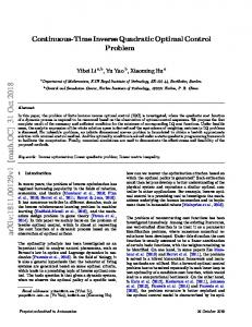
We remark that, although the factorization D = N X and the operator S are not unique, the formulas given above produce the same result independently of how the factorization is chosen. This follows from Lemma 2.4 (see, in particular, part (iv)). Theorem 2.6 (see [23, Theorem 27]). Let J = J ∗ ∈ L(Y ), and let Ψ = A B [ C D ] be a stable J-coercive well-posed linear system on (U, H, Y ). Let x0 ∈ H, let xopt (x0 ), y opt (x0 ), and uopt (x0 ) be the optimal state, output, and control for the quadratic cost minimization problem, and let Π be the corresponding Riccati operator (see Lemma 2.5). (i) Let D = N X be a (J, S)-inner-outer factorization of D, and define M = X −1 . Then     K F = −S −1 π+ N ∗ JC (I − X ) is a stable and stabilizing state feedback pair for Ψ [23, Definition 22] and    opt    A(t) + BMτ (t)K x (t, x0 ) A (t)  x0  y opt (x0 )  =  C  x0 =  C + NK K MK uopt (x0 )     A(t) BMτ (t) =  C  x0 −  N  S −1 π+ N ∗ JCx0 0 M is equal to the state and output of the closed loop system Ψ defined by     A + Bτ MK   BM  A   B   N D  =  C + N K Ψ =  C F MK K M−I

with initial value x0 , initial time zero, and zero control u (see Figure 2.1). The Riccati operator Π of Ψ can be written in the following alternative forms: ∗ ∗ JC = C JC. Π = C ∗ JC − K∗ SK = C ∗ JC = C y opt (x )

(ii) Conversely, suppose that [uopt (x00 ) ] is equal to the observation of some stable state feedback perturbation Ψ of Ψ with initial value x0 , initial time zero, zero control u , and some admissible stable state feedback pair [K F]. Then there exists an operator S ∈ L(U ), S ≫ 0, such that N X is a (J, S)-inner-outer −1 factorization of D, where N = D (I − F) and X = (I − F). Moreover, K ∗ −1 is given by K = −S π+ N JC.

6

OLOF J. STAFFANS

x y z

r

+ π+ u + -? c

x0 ? A C K

Bτ D F 6

r

u-

Fig. 2.1. Optimal state feedback connection Ψ in Theorem 2.6.

(iii) If y = C x0 + D π+ u is the first output of the optimal closed loop system Ψ with initial state x0 ∈ H and control u ∈ L2 (R+ ; U ) (see Figure 2.1), then the closed loop cost Q (x0 , u ) is given by (2.2)

Q (x0 , u ) = hy, JyiL2 (R+ ;Y ) = hx0 , Πx0 iH + hu , Su iL2 (R+ ;Y ) .

Proof. Only (iii) requires a proof, since this identity is not found in [23]. This proof goes as follows (the last equality follows from Lemma 2.5):

 hy, JyiL2 (R+ ;Y ) = (y opt (x0 ) + N π+ u )(s), J(y opt (x0 ) + N π+ u )(s) L2 (R+ ;Y )

 = y opt (x0 ), Jy opt (x0 ) L2 (R+ ;Y )

 + 2ℜ X π+ u (s), D∗ Jy opt (x0 ) L2 (R+ ;U ) + hu , N ∗ JN π+ u iL2 (R+ ;U )

= hx0 , Πx0 iH + hu , Su iL2 (R+ ;U ) . Remark 2.7. This theorem is actually true under weaker stability assumptions. It suffices if C and D are stable, i.e., A and B need not be stable [24, Definition 2.11]. Of course, the corresponding closed loop A and B need not be stable in this case. Stability of A was not assumed in [23], and the stability of B was never used in a nontrivial way in the proofs (although it was assumed). See also [33] which requires no stability of A and B. Remark 2.8. The conclusion of part (iii) of Theorem 2.6 says that the frequency response of the input/output map from the closed loop control u in Figure 2.1 to the original output is completely flat, i.e., this input/output map is all-pass, with a power amplification level equal to S. Thus, S measures the sensitivity of the closed loop system with respect to deviations from the optimal strategy. This is the reason why we call S the sensitivity operator of the closed loop system. 3. Quadratic cost minimization: Reduction to the stable case. We are now ready to attack the unstable quadratic cost minimization problem. The definition of the problem is essentially the same as in the stable case. B Definition 3.1. Let Ψ = [ A C D ] be a well-posed linear system on (U, H, Y ), and ∗ let J = J ∈ L(Y ). The (nonstandard) quadratic cost minimization problem for Ψ with cost operator J consists of finding, for each x0 ∈ H, the infimum of the cost Q(x0 , u) defined in (2.1) over all those u ∈ L2 (R+ ; U ) for which the corresponding observation y = Cx0 + Dπ+ u of Ψ satisfies y ∈ L2 (R+ ; Y ). If there exists an operator Π = Π∗ ∈ L(H) such that the optimal cost is given by inf

u∈L2 (R+ ;U )

Q(x0 , u) = hx0 , Πx0 iH ,

QUADRATIC OPTIMAL CONTROL

7

then Π is called the Riccati operator of Ψ with cost operator J. Clearly, Q is a quadratic, possibly unbounded, function of u ∈ L2 (R+ ; U ) due to the fact that Dπ+ is a linear, possibly unbounded, operator in L2 (R+ ; U ). The latter operator is not bounded on L2 (R+ ; U ) unless Ψ is input-output stable, but it is always closed. Lemma 3.2. Let D ∈ T ICα (U ; Y ) for some α ≥ 0. Then the restriction D0 of the Toeplitz operator Dπ+ to the domain  dom(D0 ) = u ∈ L2 (R+ ; U ) | Dπ+ u ∈ L2 (R+ ; Y ) is a closed (possibly unbounded) linear operator from dom(D0 ) ⊂ L2 (R+ ; U ) into L2 (R+ ; Y ). Proof. This follows directly from the fact that L2 (R+ ) is continuously imbedded in L2α (R+ ). We can say something more about how D0 maps L2 (R+ ; U ) into L2 (R+ ; Y ) in the case where D has a right coprime factorization.4 Lemma 3.3. Let D ∈ T ICα (U ; Y ) for some α ≥ 0, and suppose that D has a right coprime factorization (N , M) [24, Definition 4.2]. (i) If u ∈ L2loc (R+ ; U ), u♭ ∈ L2loc (R+ ; Y ), and y ∈ L2loc (R+ ; Y ) satisfy u = Mπ+ u♭ and y = N π+ u♭ , 2

+

then u♭ ∈ L (R ; U ) iff both u ∈ L2 (R+ ; U ) and y ∈ L2 (R+ ; Y ). Thus, dom(D0 ) is equal to the image of L2 (R+ ; U ) under Mπ+ , and range(D0 ) is equal to the image of L2 (R+ ; U ) under N π+ . In particular, dom(D0 ) is dense in L2 (R+ ; U ) iff M is outer. (ii) With u, u♭ , and y as above, there exist strictly positive constants ǫ and M such that
ǫ kuk2L2 (R+ ;U ) + kyk2L2 (R+ ;Y ) ≤ ku♭ k2L2 (R+ ;U )
≤ M kuk2L2 (R+ ;U ) + kyk2L2 (R+ ;Y ) .

Proof. Clearly, if u♭ ∈ L2 (R+ ; U ), then both u ∈ L2 (R+ ; U ) and y ∈ L2 (R+ ; Y ). Conversely, if both u ∈ L2 (R+ ; U ) and y ∈ L2 (R+ ; Y ), then we can use the right coprimeness of N and M to write
e + Xeu, e + XeM π+ u♭ = Yy u♭ = YN

and this implies that u♭ ∈ L2 (R+ ; U ). The claims about the domain and range of D0 follow immediately, and so does claim (ii). As a special case of this result (take N = D and M = I) we get the following (trivial) estimate. Lemma 3.4. For each D ∈ T IC(U ; Y ) there exist strictly positive constants ǫ and M such that, for all u ∈ L2 (R; U ),
ǫ kuk2L2 (R;U ) + kDuk2L2 (R;Y ) ≤ kuk2L2 (R;U ) ≤ kuk2L2 (R;U ) + kDuk2L2 (R;Y ) .

A necessary and sufficient condition for the existence of a finite infimum for the nonstandard quadratic cost minimization problem is that the cost function Q is bounded from below as a function of u. This should be true for each fixed x0 ∈ H. We shall actually impose a slightly stronger condition on Q which implies that not only does the infimum exist, but it is in fact a minimum.5 However, before intro4 This is true, e.g., when D is the input-output map of a jointly stabilizable and detectable well-posed linear system. See [24, Theorem 4.4]. 5 See Lemma 3.9.

8

OLOF J. STAFFANS

ducing this condition, let us make the following simple observation about the stable case. Lemma 3.5. Let J = J ∗ ∈ L(Y ). The operator D ∈ T IC(U ; Y ) is J-coercive iff D∗ JD ≥ ǫ(D∗ D + I) for some ǫ > 0, i.e., hDu, JDuiL2 (R;Y ) ≥ ǫ kuk2L2 (R;U ) +
kDuk2L2 (R;U ) for all u ∈ L2 (R; U ). Proof. This follows from Definition 2.2 and Corollary 3.4. In the unstable case we turn the characterization of J-coercivity given in this lemma into a definition. Definition 3.6. Let J = J ∗ ∈ L(Y ), and let α ≥ 0. (i) The operator D ∈ T ICα (U ; Y ) is J-coercive iff there exists a constant ǫ > 0 such that   2 2 hDπ+ u, JDπ+ uiL2 (R+ ;Y ) ≥ ǫ kukL2 (R+ ;U ) + kDπ+ ukL2 (R+ ;Y ) for all those u ∈ L2 (R+ ; U ) for which Dπ+ u ∈ L2 (R+ ; Y ). B (ii) The system Ψ = [ A C D ] on (U, H, Y ) is J-coercive if there exist constants M > 0 and ǫ > 0 such that the cost function Q defined in (2.1) satisfies   2 2 2 (3.1) Q(x0 , u) ≥ ǫ kukL2 (R+ ;U ) + kykL2 (R+ ;Y ) − M kx0 kH

for all those x0 ∈ H and u ∈ L2 (R+ ; U ) for which y = Cx0 + Dπ+ u ∈ L2 (R+ ; Y ). By Lemma 3.5, part (i) of Definition 2.2 is consistent with part (i) of Definition 3.6. That the second half of these definitions is also consistent follows from the next lemma. Lemma 3.7. A stable system is J-coercive in the sense of Definition 3.6 iff its input-output map is J-coercive.6 Proof. Trivially, the J-coercivity of an arbitrary system (stable or not) implies that its input-output map is J-coercive (take x0 = 0). Conversely, suppose that D is J-coercive, e.g., in the sense of Definition 2.2. For each u ∈ L2 (R+ ; U ) we have hDπ+ u + Cx0 , J(Dπ+ u + Cx0 )iY 2

2

≥ hDπ+ u, J(Dπ+ u)iY − 2 kJk kDk kCk kuk kx0 k − kJk kCk kx0 k . Combining this with Lemma 3.5 and with the fact that for all positive constants a, b, and δ it is true that 2ab ≤ δa2 + (1/δ)b2 , we find that for some sufficiently large constant M , independent of u and x0 , 2

2

hDπ+ u + Cx0 , J(Dπ+ u + Cx0 )iY ≥ ǫ/2(kuk + kyk2 ) − M kx0 k . Thus, the system is J-coercive in the sense of Definition 3.6. Lemma 3.8. Let J = J ∗ ∈ L(U ; Y ), and let D ∈ T ICα (U ; Y ) for some α ≥ 0. If D has a right coprime factorization (N , M), then D is J-coercive iff N is J-coercive. Proof. This follows from Lemmas 3.3 and 3.5 and Definition 3.6. Our approach to the quadratic cost minimization problem is to first use a preliminary stabilizing feedback and to then minimize the stabilized problem. It is based on the following result. 6 The same statement is actually true for all jointly stabilizable and detectable systems. See Lemma 3.9(iii).

QUADRATIC OPTIMAL CONTROL

9

B Lemma 3.9. Let J = J ∗ ∈ L(Y ), and let Ψ = [ A C D ] be a well-posed linear system on (U, H, Y ) with jointly stabilizing feedback and output injection pairs [K1 F 1 ] and [H G ] [24, Definition 3.15]. Let   A♭   B♭  D♭  Ψ♭ =  C♭ F♭1 K♭1 
−1 1
−1  K # " B I − F1 A + Bτ I − F 1 "
−1 #
−1 1  =  C + D I − F1  D I − F1 K
−1 1
−1 I − F1 K I − F1 −I

be the state feedback perturbed version of Ψ [24, Lemma 3.13] with feedback pair [K1 F 1 ]. (i) The output y = Cx0 + Dπ+ u of Ψ with initial value x0 ∈ H and control u ∈ L2loc (R+ ; U ) is equal to the first output y = C♭ x0 + D♭ π+ u♭ of Ψ♭ with the same initial value x0 ∈ H and control u♭ ∈ L2loc (R+ ; U ) if we choose u and u♭ to satisfy

−1 1
(3.2) u = I − F1 K x0 + π+ u♭ = K♭1 x0 + I + F♭1 π+ u♭ , or equivalently,7


u♭ = −K1 x0 + I − F 1 π+ u.

With this choice of u and u♭ , the states x(t) = A(t)x0 + Bτ (t)π+ u and x(t) = A♭ (t)x0 + B♭ τ (t)π+ u♭ of the two systems are also equal for all t ∈ R+ . Moreover, u♭ ∈ L2 (R+ ; U ) iff both y ∈ L2 (R+ ; Y ) and u ∈ L2 (R+ ; U ), and there exists a constant M (independent of x0 , u, and u♭ ) such that   2 2 2 kukL2 (R+ ;U ) ≤ M kx0 kH + ku♭ kL2 (R+ ;U ) ,   2 2 2 2 ku♭ kL2 (R+ ;U ) ≤ M kx0 kH + kykL2 (R+ ;Y ) + kukL2 (R+ ;U ) .

(ii) The original system Ψ is J-coercive iff the feedback stabilized system Ψ♭ is so. (iii) The original system Ψ is J-coercive iff its input/output map D is J-coercive. (iv) If either (hence both) of the two systems is J-coercive, then the controls u ∈ L2 (R+ ; U ) of Ψ and u♭ ∈ L2 (R+ ; U ) of Ψ♭ are uniquely determined by the initial state x0 and the (first) output y. In particular, if the output y = Cx0 + Dπ+ u of Ψ with initial value x0 and control u ∈ L2 (R+ ; U ) is equal to the first output C♭ x0 + D♭ π+ u♭ of Ψ♭ with initial value x0 and control u♭ ∈ L2 (R+ ; U ), then u and u♭ must satisfy (3.2). Proof. (i) The output of Ψ is given by y = Cx0 + Dπ+ u and the first output of Ψ♭ is given by y = C♭ x0 + D♭ u♭ = (C + D(I − F 1 )−1 K1 )x0 + D(I − F 1 )−1 π+ u♭ , so we get the same output if we let u and u♭ satisfy (3.2). By [24, Theorem 4.4], (D♭ , (I + F♭1 )) is a right coprime factorization of D. Since it is possible to write the equations connecting u, u♭ , and y in the form
u = I + F♭1 π+ u♭ + K♭1 x0 , y = D♭ π+ u♭ + C♭ x0 , 7 See

the equivalent [24, Figures 3.4 and 3.7].

10

OLOF J. STAFFANS

and since (by the stability of Ψ♭ ) K♭ x0 ∈ L2 (R+ ; U ) and C♭ x0 ∈ L2 (R+ ; Y ), it follows from Lemma 3.3 that u♭ ∈ L2 (R+ ; U ) iff both y ∈ L2 (R+ ; Y ) and u ∈ L2 (R+ ; U ). Moreover, the listed inequalities are true. (ii) Suppose that Ψ is J-coercive. By the second of the two inequalities in part (i), 2

2

2

2

ǫ/2 kukL2 (R+ ;U ) + ǫ/2 kykL2 (R+ ;Y ) ≥ −ǫ/2 kx0 kH + ǫ/(2M ) ku♭ kL2 (R+ ;U ) , and this combined with (3.1) implies that Ψ♭ is J-coercive (replace M by M + ǫ/2 and ǫ by min{ǫ/2, ǫ/(2M )}). The proof of the converse part is similar but simpler. (iii) This follows from part (ii) and Lemmas 3.7 and 3.8. (iv) If the two controls u1♭ and u2♭ produce the same output y = C♭ x0 + D♭ u1♭ = C♭ x0 + D♭ u2♭ , then their difference u1♭ − u2♭ satisfies D♭ π+ (u1♭ − u2♭ ) = 0. As D♭ is J-coercive, D♭ π+ is one-to-one on L2 (R+ ; U ), and we find that π+ (u1♭ − u2♭ ) = 0. Similarly, if the two controls u1 and u2 produce the same output y = Cx0 + Dπ+ u1 = Cx0 + Dπ+ u2 , then their difference u1 − u2 satisfies Dπ+ (u1 − u2 ) = 0. Define z = (I + F♭1 )−1 π+ (u1 − u2 ). Then (I + F♭1 )z = u1 − u2 and D♭ z = D(u1 − u2 ) = 0. Recall that (D♭ , (I + F♭1 )) is a right coprime factorization of D [24, Theorem 4.4]. From Lemma 3.3 we conclude that z ∈ L2 (R+ ; U ), which combined with the Jcoercivity of D♭ implies that z = 0. Thus, u1 − u2 = 0 also. 4. The solution to the unstable quadratic cost minimization problem. Lemma 3.9 gives us the following preliminary solution to the general quadratic cost minimization problem. B Lemma 4.1. Let J = J ∗ ∈ L(Y ), and let Ψ = [ A C D ] be a jointly stabilizable and detectable J-coercive well-posed linear system on (U, H, Y ). Then the quadratic cost minimization problem with cost operator J has a unique minimizing solution uopt (x0 ) ∈ L2 (R+ ; U ). This solution can be computed as follows: We first feedback stabilize Ψ as described in Lemma 3.9, and we then apply Lemma 2.5 with Ψ replaced by the stabilized system Ψ♭ to get an optimal control uopt ♭ (x0 ), an optimal output y opt (x0 ), and an optimal state trajectory xopt (x0 ) for the stabilized system. The optimal control for the original system Ψ is then given by uopt (x0 ) = K♭1 x0 + (I + F♭1 )π+ uopt ♭ (x0 ), and the optimal output and state for the original minimization problem is equal to the optimal output y opt (x0 ) and state xopt (x0 ) for the stabilized minimization problem. In particular, the original problem and the stabilized problem have the same Riccati operator. The solution given by Lemma 4.1 is not yet complete in the sense that it does not contain the same type of feedback description as Theorem 2.6 does for the stable case. Our next task will be to develop such a feedback description. This description will be given in terms of a right coprime factorization of the input/output map D with the special property that its numerator is (J, S)-inner. This notion is defined as follows. Definition 4.2. Let J = J ∗ ∈ L(Y ), let S = S ∗ ∈ L(U ) be invertible, let D ∈ T ICα (U ; Y ) for some α ≥ 0, and let (N , M) be a right coprime factorization of D in T IC. (i) If N is (J, S)-inner, then (N , M) is a (J, S)-inner right coprime factorization of D. N ] is (I, S)-inner, i.e., if N ∗ N + M∗ M = S, then (N , M) is an S(ii) If [ M normalized right coprime factorization of D. Lemma 4.3. Let J = J ∗ ∈ L(Y ), and let S ∈ L(U ), S ≫ 0, Se ∈ L(U ), and Se ≫ 0. Let D ∈ T ICα (U ; Y ) for some α ≥ 0, and suppose that D has a right coprime factorization (N , M) in T IC(U ; Y ).

QUADRATIC OPTIMAL CONTROL

11

(i) If D is stable, then (N , M) is a (J, S)-inner right coprime factorization of D iff N M−1 is a (J, S)-inner-outer factorization of D, or equivalently, iff M−1 is an S-spectral factor of D∗ JD. (ii) D has a (J, S)-inner right coprime factorization iff D is J-coercive. (iii) The set of all possible (J, S)-inner right coprime factorizations (N , M) of D (where J and D are fixed while N , M and S vary) can be parameterized as e f is a fixed (J, S)-inner e , M) e where (N f and S = E ∗ SE, e E, M = ME, N =N right coprime factorization of D and E ∈ L(U ) is an arbitrary invertible operator. Proof. (i) It is easy to see that if X is an S-spectral factor of D∗ JD, and if we define M = X −1 and N = DX , then (N , M) is a (J, S)-inner right coprime factorization of D (it is coprime since M is invertible in T IC(U )). Conversely, if (N , M) is a (J, S)-inner right coprime factorization of D, then (D, I) is another right coprime factorization of D, and it follows from [24, Lemma 4.3(i)] that M has an inverse in T IC(U ). It is then obvious that X = M−1 is an S-spectral factor of D∗ JD. (ii) If D is J-coercive, then by Lemmas 3.8 and 2.4(i), N is J-coercive and has a e X . According to Lemma 2.4(ii), X is invertible, (J, S)-inner-outer factorization N = N f e and by [24, Lemma 4.3(i)], (N , M) = (N X −1 , MX −1 ) is a (J, S)-inner right coprime factorization of D. On the other hand, if D has a (J, S)-inner right coprime factorization (N , M), then N is (J, S)-inner, hence J-coercive (since we assume that S ≫ 0). By Lemma 3.8, D is J-coercive. (iii) This follows from [24, Lemma 4.3(i)] and Lemma 2.4(iii). The following is our first main result. B Theorem 4.4. Let J = J ∗ ∈ L(Y ), let S ∈ L(U ), S ≫ 0, and let Ψ = [ A C D ] be a J-coercive jointly stabilizable and detectable well-posed linear system on (U, H, Y ) [24, Definition 3.16]. Let xopt (x0 ), y opt (x0 ), and uopt (x0 ) be the optimal state, output, and control for the quadratic cost minimization problem for Ψ, and let Π be the corresponding Riccati operator (cf. Lemma 4.1). (i) Let (N , M) be a (J, S)-inner right coprime factorization of D. Then there is a unique feedback map K such that [K F] = [K (I − M−1 )] is an admissible stabilizing state feedback pair for Ψ and     opt   A(t) + BMτ (t)K x (t, x0 ) A (t)  x0  y opt (x0 )  =  C  x0 =  C + NK K MK uopt (x0 ) is equal to the state and output of the closed loop system Ψ defined by     A + Bτ MK A   B    BM   D  =  C + N K N Ψ =  C F K MK M−I

with initial value x0 , initial time zero, and zero control u (see Figure 2.1). The feedback map K is uniquely determined by the fact that C = C + N K ∈ L(H; L2 (R+ ; Y )), K = MK ∈ L(H; L2 (R+ ; U )), and π+ N ∗ JC = 0. Moreover, the Riccati operator of Ψ is given by ∗ JC = (C + N K)∗ J(C + N K). Π = C

12

OLOF J. STAFFANS

(ii) If y = C x0 + D π+ u is the first output of the optimal closed loop system Ψ in (i) with initial state x0 ∈ H and control u ∈ L2 (R+ ; U ) (see Figure 2.1), then the closed loop cost Q (x0 , u ) is given by (4.1)

Q (x0 , u ) = hy, JyiL2 (R+ ;Y ) = hx0 , Πx0 iH + hu , Su iL2 (R+ ;Y ) .

(iii) If Ψ is jointly ω-stabilizable and detectable for some ω < 0 [24, Definition 3.16], and if N and M in (i) are right ω-coprime [24, Definition 4.1], then the closed loop system Ψ is ω-stable. (iv) If (N , M) are given, then the feedback map K, the Riccati operator Π, the closed loop semigroup A , and the closed loop controllability and feedback maps C and K can be computed as follows: Choose some arbitrary jointly stabilizing feedback and output injection pairs [K1 F 1 ] and [ H G ]. Then K = M−1 K1 − S −1 π+ N ∗ JC♭ ,      ♭  BMτ A♭ A  C  =  C♭  −  N  S −1 π+ N ∗ JC♭ , M K♭1 K

∗ ∗ Π = C♭ JC♭ − K − M−1 K♭1 S K − M−1 K♭1
∗ JC♭ , = C♭∗ J − JN S −1 π+ N ∗ J C♭ = C♭∗ JC = C

where A♭ = A + Bτ K♭1 , C♭ = C + DK♭1 , and K♭1 = (I − F 1 )−1 K1 . (If Ψ is stable, then we can can take K♭1 = 0, A♭ = A, and C♭ = C and get the same formulae as in Theorem 2.6). Proof. Let us first show that the conditions on K in (i) determine K uniquely. Suppose that we have two feedback maps K1 and K2 such that both C +N K1 and C +N K2 belong to L(H; L2 (R+ ; Y )), both MK1 and MK2 belong to L(H; L2 (R+ ; U )), and π+ N ∗ J(C + N K1 ) = π+ N ∗ J(C + N K2 ). Then, for each x ∈ H, N (K1 − K2 )x ∈ L2 (R+ ; Y ), M(K1 − K2 )x ∈ L2 (R+ ; U ), and π+ N ∗ J(N (K1 − K2 )x) = 0. By Lemma 3.3, (K1 − K2 )x ∈ L2 (R+ ; U ), hence 0 = π+ N ∗ J(N (K1 − K2 )x) = π+ (N ∗ JN )(K1 − K2 )x = Sπ+ (K1 − K2 )x. As (K1 − K2 )x is supported on R+ and S invertible, we must have (K1 − K2 )x = 0 for all x ∈ H. In order to prove the remainder of (i) we proceed as suggested by (iv); i.e., we choose preliminary jointly stabilizing feedback and output injection pairs [K1 F 1 ] and [ H G ] with interaction operator E1 . The output injection pair and the interaction operator E1 play a very nonsignificant role below; they are only needed so that we can apply [24, Theorem 4.4] in order to show that (D(I − F 1 )−1 , (I − F 1 )−1 ) is a right coprime factorization of D. We shall therefore ignore the output injection part of the system for the rest of this proof, but we return to this question at the end of the section. We add the state feedback pair [K1 F 1 ] to the system Ψ and close the state feedback loop as in Lemma 3.9 to get the stable system Ψ♭ given in that lemma. According to Lemma 4.1, the quadratic cost minimization problems for Ψ and Ψ♭ have the same optimal state xopt (x0 ) and output y opt (x0 ) and the optimal controls uopt (x0 ) and uopt ♭ (x0 ) are related to each other as in (3.2). We want to apply Theorem 2.6 to solve the quadratic cost minimization problem for the closed loop system Ψ♭ . By Lemmas 3.7 and 3.9, D♭ is coercive. Since both

QUADRATIC OPTIMAL CONTROL

13

(D♭ , (I + F♭1 )) and (N , M) are right coprime factorizations of D, it follows from [24, Lemma 4.3] that the operator


−1 (4.2) X = M−1 I + F♭1 = I − F 1 M

belongs to T IC(U ) and is invertible in T IC(U ). Thus, N X is a (J, S)-inner-outer factorization of D♭ . By Theorem 2.6, the solution to the quadratic cost minimization problem for Ψ♭ is of state feedback type. More precisely, the pair     K♮ F♮ = −S −1 π+ N ∗ JC♭ (I − X ) is a stable stabilizing state feedback pair for Ψ♭ , and if we further extended the system Ψ♭ into   A♭   B♭   C♭ D♭    1 K  F 1  ♭ ♭ F♮ K♮

by adding the extra state feedback pair, and then close the new state feedback loop to get the stable closed loop system [24, Lemma 4.5]   A♭   B♭   C♭ D♭   Ψ♭ =  1   1  K♭ F♭ F♮ K♮   −1 −1 A♭ + B♭ τ X−1 K♮  B♭ X −1    C♭ + D♭ X K♮ D♭ X  = K1 + F 1 X −1 K♮   F 1 X −1  ♭ ♭ ♭ X −1 − I X −1 K♮
  1 BM A + Bτ K1♭ + MK♮
     C + D K + MK♮ N ♭ , = 1   K1 + F 1 MK♮    M F ♭

1 1 I −F M−I I − F MK♮

then xopt (x0 ), y opt (x0 ), and uopt ♭ (x0 ) are given by
    opt   x (x0 ) A + Bτ K♭1 + MK♮
A♭ y opt (x0 ) =  C♭  x0 =  C + D K1 + MK♮  x0 ♭
1 K I − F MK♮ ) (x uopt ♮ 0 ♭ and C♭ satisfies

N ∗ JC♭ = 0. From this result we are able to derive the conclusions listed in (i) and (iv). Most of the proof is ready. In particular, the formulae for the Riccati operator Π given in (iv) follow from Lemma 3.9 and the corresponding formulae in Theorem 2.6. It only remains to return to the original system Ψ and the original control uopt (x0 ). The optimal control uopt ♭ (x0 ) for Ψ♭ corresponds to the optimal control uopt (x0 ) = I − F 1


−1



1 K1 x0 + uopt ♭ (x0 ) = K♭ + MK♮ x0

14

OLOF J. STAFFANS

for the original system Ψ. We observe that uopt (x0 ) is equal to the sum of the two last outputs of Ψ♭ with zero control. Let us add these two rows and combine them into one to get the system     A + Bτ MK   BM  A   B  , N D  =  C + N K Ψ =  C MK M−I F K where K = M−1 K = K♮ + M−1 K♭1 . We then have

      opt A(t) + BMτ (t)K A (t) x (t, x0 )  x0 .  y opt (x0 )  =  C  x0 =  C + NK MK K uopt (x0 )

Moreover, since C = C♭ , we have N ∗ JC = 0, and Ψ is the system that we get by closing the state feedback loop in the system   A  B   C D , K F

where K is the feedback map defined above and F = I − M−1 . This completes the proofs of both (i) and (iv). The proof of (ii) is identical to the proof of Theorem 2.6(iii). Finally, let us prove (iii). Under the assumption of (iii) we can throughout work with the notion of ω-stability instead of just plain stability (the latter notion is the same as ω-stability with ω = 0). The only part of the extended optimal system Ψ♭ whose ω-stability is not obvious is the state feedback map K♮ ; all the other parts of the system are bounded linear operators on the correct spaces. Thus, we must show that K♮ ∈ L(H; L2ω (R+ ; U )). Recalling the definition of K♮ , we realize that it suffices to show that the anticausal operator N ∗ belongs to T Iω (Y ; U ). Here the duality is with respect to the inner product in the unweighted L2 , so by standard duality theory N ∗ ∈ T I−ω (Y ; U ). However, since N ∗ is anticausal, this implies that N ∗ can be extended to an anticausal operator in T Iβ (Y ; U ) for all β ≤ −ω [24, Lemmas 2.4 and 2.9]. In particular, since ω ≤ 0, N ∗ ∈ T Iω (Y ; U ). Thus, K♮ ∈ L(H; L2ω (R+ ; U )), and Ψ♭ is stable. Remark 4.5. An inspection of the proof of Theorem 2.6 shows that if the system Ψ is jointly strongly stabilizable and detectable, then the optimal closed loop system Ψ will be strongly stable, too [24, Lemma 3.5]. Theorem 4.4 does not contain a converse part like the one found in Theorem 2.6(ii), since we have been able to prove only the following partial converse. Theorem 4.6. Make the same hypothesis as in Theorem 4.4. Suppose that the solution to the quadratic cost minimization problem is of state feedback type in opt 0) the sense that [ uy opt(x (x0 ) ] is equal to the output of the closed loop system Ψ with initial value x0 , initial time zero, zero input u , and some stabilizing state feedback pair [K F]. Define M = (I − F)−1 and N = DM. Then there exists a positive invertible operator S = S ∗ ∈ L(U ) such that N is (J, S)-inner, and the claim (ii) in Theorem 4.4 is true for this closed loop system. If, moreover, N and M are right coprime, then (N , M) is a (J, S)-inner right coprime factorization of D. This is true, in particular, whenever Ψ is exponentially stabilizable.

QUADRATIC OPTIMAL CONTROL

15

Proof. We suppose that the solution to the quadratic cost minimization problem for Ψ is of state feedback type and claim that this implies that the solution to the quadratic cost minimization problem for the system Ψ♭ considered in the proof of Theorem 4.4 is also of state feedback type. The proof of this is based on [24, Lemma 4.5] and Lemma 3.9. We consider the combined system   A  B   C D    1 K  F 1  , K F where (K1 , F 1 ) is the same preliminary feedback pair that we used in the proof of Theorem 4.4 and [K F] is the optimal feedback pair. By [24, Lemma 4.5], [K F] is a stabilizing feedback pair for this combined system (due to the coprimeness of D(I − F 1 )−1 and (I − F 1 )−1 ). Moreover, the pair     K♮ F♮ = K − (I − F)(I − F 1 )−1 K1 I − (I − F)(I − F 1 )−1

is a stabilizing feedback pair for Ψ♭ . By combining this fact with Lemma 3.9, we find that the optimal solution to the quadratic cost minimization problem for the system Ψ♭ is of state feedback type. However, in contrast to the situation covered by the converse part of Theorem 2.6, we do not know that the feedback pair [K♮ F♮ ] itself is stable, and this causes some additional complications and prevents us from applying part (ii) of Theorem 2.6. Instead we argue directly, examining the proof of the converse part of Theorem 2.6 as presented in [23]. We know that F♮ ∈ T ICα (U ) for some α ≥ 0 (but not necessarily for α = 0) and that (I −F♮ )−1 ∈ T IC(U ). Fortunately, it was the latter property that was important for a major part of the proof of Theorem 2.6(ii). By repeating the argument in [23] we find that if we define M♮ = (I − F♮ )−1 , then M∗♮ D♭∗ JD♭ M♮ = S for some nonnegative S = S ∗ ∈ L(U ). However, the proof given there of the invertibility of S was based on the boundedness of F♮ , so it does not apply. Since M♮ is invertible in T ICα (U ), we know that M♮ is one-to-one. This together with the invertibility of D♭∗ JD♭ (which is a consequence of the J-coercivity) implies that S is one-to-one. Its inverse S −1 is a nonnegative, possibly unbounded, selfadjoint operator which has a nonnegative self-adjoint square root S −1/2 . Denote the domain of S −1/2 by W . Then M♮ S −1/2 ∈ T IC(W ; U ), and it can be extended to an operator on T IC(U ) since S −1/2 M∗♮ D♭∗ JD♭ M♮ S 1/2 can be extended to the f Then identity operator on T IC(U ). We denote this extension of M♮ S −1/2 by M. f ∈ T ICα (W ; U ), and it can be extended to an operator in T ICα (U ) M S −1/2 = M−1 ♮ since the right-hand side of this equation belongs to T ICα (U ). But this means that S −1/2 can be extended to an operator in L(U ), hence S 1/2 and S must be invertible. Since N = DM = D(I − F)−1 = D♭ M♮−1 , and since M∗♮ D♭∗ JD♭ M♮ = S, we find that N is (J, S)-inner as claimed. The proof of the statement given in part (ii) of Theorem 4.4 remains the same as before. We have not been able to prove that N and M must always be right coprime. This will be true if and only if the feedback pair [K1 F 1 ] stabilizes the original system extended with the feedback pair [K F], cf. [24, Lemma 4.5]. In particular, it is true whenever [K1 F 1 ] is exponentially stabilizing; see [24, Lemma 3.20].

16

OLOF J. STAFFANS

x y z˜

r

π+ u -

E

+ + c -?

x0 ? A C e K

Bτ D Fe 6 r

u -

Fig. 4.1. Externally parameterized optimal state feedback system.

According to Lemmas 2.4 and 4.3, Theorems 2.6 and 4.4 contain a hidden free invertible parameter E ∈ L(U ).8 For example, the set of all possible (J, S)-inner coprime factorization of D in Theorem 4.4 can be parameterized as follows. e , M) f be a particular (J, S)-inner e Proposition 4.7. Let (N coprime factorization of D. Then the set of all possible sensitivity operators S and all possible (J, S)-inner coprime factorizations (N , M) of D (where J and D are fixed while N , M, and S vary) can be parameterized as e S = E ∗ SE,

e E, N =N

f M = ME,

where E varies over the set of all invertible operators in L(U ). The corresponding feedback pair [K F] in Theorem 4.4 is given by e K = E −1 K,

e (I − F) = E −1 (I − F),

f−1 ); i.e., [K e F] e is the feedback pair in e ∗ JC and Fe = (I − M e +N e = −Sπ where K f e Theorem 4.4 corresponding to the factorization (N , M). The parameterized version of the formula for the closed loop system in Theorem 4.4 is     e f f K A + B Mτ   B ME  A   B  e eK eE . N D  =  C + N Ψ =  C f e f MK ME − I F K

The first column is independent of E (but the second is not). This follows from Lemma 4.3. The operator E has a very simple interpretation: it represents a coordinate change in the input space for the closed loop system. Proposition 4.8. Introduce the same notation as in Proposition 4.7. Then the two diagrams drawn in Figures 2.1 and 4.1 are equivalent in the sense that the relationships between all the signals with identical names are identical in the two diagrams (but z differs in general from z˜.) Proof. Clearly, if we can show that the relationships between u and u are the same in both the diagrams, then all the other relationships will be the same, too, since both diagrams say that x = Ax0 + Bτ u, y = Cx0 + Du.

8 In [23] this parameter was written out explicitly and it was explained why it cannot be avoided: it represents an undetermined feed-forward term inside the feedback loop.

QUADRATIC OPTIMAL CONTROL

17

In Figure 2.1 we have u = Kx0 + Fu + π+ u♭ , from which we can solve u in the form −1

u = (I − F) (Kx0 + π+ u♭ )
e 0 + π+ u ♭ e −1 E E −1 Kx = (I − F) e 0 + Eπ+ u♭ ) . e −1 (Kx = (I − F)

On the other hand, Figure 4.1 says that

e + Eπ+ u♭ , e 0 + Fu u = Kx

and this equation is equivalent to the one above. The minimization problem considered in Theorem 4.4 leads to an inner coprime factorization. If instead we use the different cost function (4.3)

2

2

Q1 (x0 , u) = kykL2 (R+ ;Y ) + kukL2 (R+ ;U ) ,

then we get a normalized coprime factorization. B Corollary 4.9. Let Ψ = [ A C D ] be a jointly stabilizable and detectable well-posed opt linear system on (U, H, Y ). Let x (x0 ), y opt (x0 ), and uopt (x0 ) be the optimal state, output, and control for the quadratic cost minimization problem described in Definition 3.1, but with the cost function Q(x0 , u) replaced by the cost function Q1 (x0 , u) in (4.3). If S = S ∗ ∈ L(U ) and (N , M) is an S-normalized right coprime factorization of D (in the sense of Definition 4.2), then there is a unique feedback map K such that
[K F] = [K I − M−1 ] is an admissible stabilizing state feedback pair for Ψ and     opt   A(t) + BMτ (t)K A (t) x (t, x0 )  x0  y opt (x0 )  =  C  x0 =  C + NK opt K MK u (x0 ) is equal to the state and output  A  Ψ =  C K

of the closed loop system Ψ defined by    A + Bτ MK  B    BM   D  =  C + N K N F MK M−I

with initial value x0 , initial time zero, and zero input u (see Figure 2.1). The feedback map K is uniquely determined by the fact that C = C + N K ∈ L(H; L2 (R+ ; Y )), K = MK ∈ L(H; L2 (R+ ; U )), and π+ (N ∗ C + M∗ K ) = 0. Moreover, the Riccati operator of Ψ is given by ∗ ∗ Π = C C + K K = (C + N K)∗ (C + N K) + (MK)∗ (MK).

Proof. Apply Theorem 4.4 with Ψ replaced by the augmented system   A  B  D , Ψaug =  C 0 I

18

OLOF J. STAFFANS

and use the fact that (N , M) is an S-normalized right coprime factorization of D N ], M) is an (I, S)-inner right coprime factorization of [ D ]. Also observe iff ([ M I that the augmented system is always coercive. The net effect is that throughout one C♭ C N C replaces J by I, D by [ D I ], N by [ M ], C by [ 0 ], C♭ by [ K♭1 ], and C by [ K ] in Theorem 4.4. Let us end this section with a discussion of the joint stabilizability and detectability assumption in Theorem 4.4. This assumption was needed so that we could apply [24, Theorem 4.4] and conclude that the preliminary feedback gives us a coprime factorization of the input/output map. The optimal feedback given by Theorem 4.4 gives us another stabilizing feedback pair. However, we are not able to prove that the optimal feedback pair and the original stabilizing output injection pair [ H G ] are jointly stabilizing (and we do not even expect this to be true in full generality). The problem is that these two pairs need not have a well-defined interaction operator E. By using the fact that the interaction operator E is determined (modulo a static part) by its Hankel operator KH, it is possible to construct E (whenever such an interaction operator exists). To do this we have to take a closer look at the proof of Theorem 4.4. The critical step in the proof is the addition of the state feedback row to the preliminary stabilized system Ψ♭ . Let us redo this part of the proof, restoring the omitted output injection column   H  G  E1 to the system Ψ1 ; i.e., let us start with the full system     A  H B  G D  Ψext =  C 1 E1 F 1 K

and close the state feedback loop to get the stable system    A♭   H♭ B♭  G♭ D♭  Ψ♭ =  C♭ E1♭ F♭1 K♭1 h 
−1 1
−1
−1 i  K A + Bτ I − F 1 H + B I − F1 E1 B I − F 1 "
−1 #
−1
−1 1 # " . = E1 D I − F 1 K G + D I − F1  C + D I − F1 


−1 −1 −1 1 E1 I − F1 −I K I − F1 I − F1

To this system we want to add a new state feedback row [K♮ E♮ this row should be constructed we examine the feedback pair     K♮ F♮ = −S −1 π+ N ∗ JC♭ (I − X ) that we used in the proof of Theorem 4.4. Since

X = M−1 (I − F 1 )−1 = S −1 N ∗ JN M−1 (I − F 1 )−1 = S −1 N ∗ JD(I − F 1 )−1 = S −1 N ∗ JD♭ , this pair can be rewritten in the alternative form      K♮ F♮ = 0 I − S −1 π+ N ∗ JC♭

 N ∗ JD♭ ,

F♮ ]. To see how

QUADRATIC OPTIMAL CONTROL

19

which gives us a clue to the correct definition of E♮ . B Lemma 4.10. Let Ψ = [ A C D ] be a stable well-posed linear system on (U, H, Y ), ∗ and let N ∈ T I(Y ; Z) be anticausal. Define K = π+ N ∗ C,

E = N ∗ D.

(i) The map K satisfies KA(t) = π+ τ (t)K,

t ∈ R+ ,

and the Hankel operator of E is given by π+ Eπ− = KB. (ii) If E can be written as a sum E = E− + E+ , where both E− and E+ belong to T I(Y ; Z) and E+ is causal and E− anticausal, then   A  B   C D  E+ K

is a stable well-posed linear system on (U, H, Y × Z). (iii) Conversely, if there exists some E+ for which the system above is a stable wellposed linear system on (U, H, Y × Z), then we get a splitting E = E− + E+ of the type described above by defining E− = E − E+ . This splitting is unique modulo a static operator E. Proof. (i) To compute KA(t) we use the anticausality and time invariance of N ∗ and part (iii) of [24, Definition 2.1] to get KA(t) = π+ N ∗ CA(t) = π+ N ∗ π+ τ (t)C = π+ N ∗ τ (t)C = π+ τ (t)N ∗ C = π+ τ (t)π+ N ∗ C = π+ τ (t)K. Almost the same argument, but with part (iii) of [24, Definition 2.1] replaced by part (iv), gives π+ Eπ− = π+ N ∗ Dπ− = π+ N ∗ π+ Dπ− = π+ N ∗ CB = KB. (ii) This follows immediately from part (i) and [24, Definition 2.1] (the Hankel operator of E− is zero). (iii) Clearly E− is anticausal, since E and E+ have the same Hankel operator. The uniqueness statement follows from [23, Lemma 6]. By applying this lemma to the crucial step in the proof of Theorem 4.4 (and using [24, Lemma 3.5]) we get the following addition to Theorem 4.4.

20

OLOF J. STAFFANS

Corollary 4.11. Let [ H G ] and E1 be the output injection pair and the interaction operator used in the proof of Theorem 4.4. Then the optimal state feedback ∗ pair [K F] and the output injection pair [ H G ] are jointly stabilizing iff N JG♭ = ∗ 1 −1 N J(G + (I − F ) E1 ) can be split into a causal and an anticausal part that both belong to T I(Y ; U ). We shall not need this result here and leave the proof to the reader. For completeness, let us also mention the following “dual” result, where one uses an anticausal time-invariant operator to construct a new output injection pair for a well-posed linear system. This result is needed in the solution to the “dual” quadratic optimal filtering problem. B Lemma 4.12. Let Ψ = [ A C D ] be a stable well-posed linear system on (U, H, Y ), ∗ e ∈ T I(Z; U ) be anticausal. Define and let N e ∗ π− , H = BN

(i) The map H satisfies

e ∗. E = DN

A(t)H = Hτ (t)π− ,

t ∈ R+ ,

and the Hankel operator of E is given by π+ Eπ− = CH. (ii) If E can be written as a sum E = E− + E+ , where both E− and E+ belong to T I(Z; U ) and E+ is causal and E− anticausal, then    A H B E+ D C

is a stable well-posed linear system on (Z × U, H, Y ). (iii) Conversely, if there exists some E+ for which the system above is a stable wellposed linear system on (Z × U, H, Y ), then we get a splitting E = E− + E+ of the type described above by defining E− = E − E+ . This splitting is unique modulo a static operator E. The proof of this lemma is very similar to the proof of Lemma 4.10, and we leave it to the reader. Remark 4.13. Theorem 4.4 and Corollary 4.9 remain true in the case where we minimize hy, JyiL2 (R+ ;Y ) instead, where β ∈ R is arbitrary. We must then throughout β

replace the unweighted space L2 by the weighted space L2β . In particular, the notion of an inner operator should be redefined so that it refers to the weighted space L2β , and the adjoints should be computed with respect to the inner product in the weighted space L2β . Remark 4.14. The results of this section remain valid if throughout we replace the algebra of time-invariant bounded linear operators from L2 (R; U ) into L2 (R; Y ) by various subalgebras, for example, the algebra of convolution operators induced by measures with finite total variation. The main exception is that spectral factorizations and inner-outer factorizations need not exist in all subalgebras. In particular, Theorem 4.4 remains valid. In the algebra studied in [18] spectral factorizations and inner-outer factorizations do exist and the input/output maps can always be decomposed into causal and anticausal parts, as required by Lemmas 4.10 and 4.12.

QUADRATIC OPTIMAL CONTROL

21

5. The optimal problem on a finite time interval. Our next goal is to show that the Riccati operator in Theorem 4.4 satisfies an algebraic Riccati equation involving the generating operators of the system Ψ. Two such algebraic Riccati equations were given in [23], namely the open loop and the closed loop algebraic Riccati equations. The derivation of the closed loop Riccati equation was based entirely on the properties of the optimal closed loop system, and that argument remains valid since the optimal closed loop system is stable. However, the open loop system can be unstable, and in order to derive the open loop Riccati equation we have to study the behavior of the optimal system on a finite time interval. Lemma 5.1. Make the same assumption and introduce the same notations as in Theorem 4.4. Then, for all x0 ∈ H and all t ≥ 0,
π[0,t] D∗ Jπ[0,t] C + τ (−t)B ∗ ΠA (t) = 0,
π[0,t] N ∗ Jπ[0,t] C + τ (−t)M∗ B ∗ ΠA (t) = 0, ∗ C Jπ[0,t] C + A∗ (t)ΠA (t) = Π, ∗ C Jπ[0,t] C + A∗ (t)ΠA (t) = Π.

(5.1) (5.2) (5.3) (5.4)

Proof. Fix t ≥ 0. Let us perform the minimization of the cost function Q(x0 , u) separately with respect to u1 = π[0,t] u and u2 = π[t,∞) u. To do this we write Q(x0 , u) in the form Q(x0 , u) =

Z

t

0

hy(s), Jy(s)iY ds +

Z

t

∞

hy(s), Jy(s)iY ds,

where y is the output of Ψ with initial time zero, initial value x0 , and control u. Let x be the corresponding state of Ψ. Since π[0,t] y = π[0,t] Cx0 + π[0,t] Dπ[0,t] u and π[t,∞) y = τ (−t)Cx(t) + Dπ[t,∞) u, we observe that the first term depends only on x0 and u1 and the second term only on x(t) and u2 . If we fix u1 and minimize with respect to u2 , then, because of the time invariance of the problem, the minimum is equal to hx(t), Πx(t)iH . Thus, we are left with the problem of minimizing the cost function (5.5)

Q(x0 , u) =

Z

0

t

hy(s), Jy(s)iY ds + hx(t), Πx(t)iH

with respect to u1 , where π[0,t] y is the function given above and x(t) = A(t)x0 + Bτ (t)u1 . Differentiating (5.5) with respect to u1 and setting the result to be zero we get (5.1). That also (5.2) holds follows from the time invariance and anticausality of M∗ and the fact that M∗ D∗ = N ∗ . By replacing y and x in (5.5) by y opt (x0 ) and xopt (x0 ) we find that hx0 , Πx0 iH =

Z

0

t





 y opt (x0 , s), Jy opt (x0 , s) Y ds + xopt (t, x0 ), Πxopt (t, x0 ) Y ,

from which (5.3) follows since y opt (x0 ) = C x0 and xopt (t, x0 ) = A (t)x0 . This

22

OLOF J. STAFFANS

 0

c + 6 − x∗ u∗

Π 

∗

A B∗

?  ∗ ∗  C ∗ K ∗ D F

6 Πx(t) − ? c+

 0

J 

x y z

6

r

S  r

x0 ? A C K

+ + c -?

B  D F

6

r

u -

π[0,t] u Fig. 5.1. Primal-dual connection with primal feedback.

combined with (5.1) implies that for all x0 and x1 in H, hx1 , Πx0 iH =

Z

t

h(C x1 )(s), J(C x0 )(s)iY ds + hA (t)x1 , ΠA (t)x0 iH

0

Z

t

 (Cx1 + Duopt (x1 ))(s), Jy opt (x0 , s) Y ds 0

 + A(t)x1 + Bτ (t)uopt (x1 ), Πxopt (x0 , t) H Z t h(Cx1 )(s), JC x0 (s)iY ds + hA(t)x1 , A (t)x0 iH , =

=



0

which gives us (5.4). We remark that Lemma 5.1 has been proved independently by Hans Zwart [35] under weaker assumptions. The preceding lemma can be interpreted as a result concerning the state and output of the adjoint system Ψ∗ if we use the state x multiplied by Π and the output y multiplied by J of the original system as initial value and control for Ψ. Corollary 5.2. Make the same assumption and introduce the same notations as in Theorem 4.4. Let xopt (x0 ) and y opt (x0 ) denote the optimal state and optimal output in the quadratic cost minimization problem for Ψ, and let x∗ and u∗ denote the state and output of the adjoint system Ψ∗ with initial time t > 0, initial value Πxopt (t, x0 ), and control y opt (x0 ) (see Figure 5.1 with u = 0). Then x∗ (s) = Πxopt (x0 , s) for all s ∈ [0, t] and π[0,t] u∗ = 0. The same formulae are true if instead x∗ and u∗ denote the state and output of the optimal adjoint system Ψ∗ with initial time t > 0, initial value Πxopt (t, x0 ), and control y opt (x0 ). Proof. Fix 0 ≤ s ≤ t. By the definition of the state of the adjoint system Ψ∗ , we have x∗ (s) = A∗ (t − s)Πxopt (t, x0 ) + C ∗ Jτ (s)π[s,t] y opt (x0 )


= A∗ (t − s)ΠA (t − s) + C ∗ Jτ (s)π[s,t] τ (−s)C xopt (x0 , s)
= A∗ (t − s)ΠA (t − s) + C ∗ Jπ[0,t−s] C xopt (x0 , s) = Πxopt (x0 , s),

where the last equality follows from (5.4). The same computation is valid if we replace Ψ∗ by Ψ∗ .

QUADRATIC OPTIMAL CONTROL

23

The restriction of the output of Ψ∗ to [0, t] is given by
π[0,t] u∗ = π[0,t] τ (−t)B ∗ Πxopt (t, x0 ) + D∗ Jπ[0,t] y opt (x0 ) ,

and this is zero according to (5.1). To prove the same result with Ψ∗ replaced by the optimal closed loop adjoint system Ψ∗ we argue in the same way, but replace (5.1) by (5.2). Remark 5.3. A similar result is true for nonzero inputs u to the primal and Su to the dual system (see Figure 5.1). This follows from Corollary 5.7 below, since the connection in Figure 5.3 becomes identical to the one in Figure 5.1 if we replace u in Figure 5.3 by u + z. Up to now we have in this section made only marginal use of Theorem 4.4, but the remaining results depend heavily on the characterization of the optimal feedback pair given in that theorem. We begin with the following key lemma. Lemma 5.4. Make the same assumption and introduce the same notations as in Theorem 4.4. Then, for all t ≥ 0, ∗ ∗ ΠB τ (t)π+ + π[0,t] D Jπ[0,t] D π[0,t] = Sπ[0,t] . π+ τ (−t)B ∗ JC and π+ D π− = Proof. To prove this we compute, using the facts that Π = C π+ N π− = C B , ∗ ∗ π+ τ (−t)B ΠB τ (t)π+ + π[0,t] D Jπ[0,t] D π[0,t] ∗ ∗ ∗ = π+ τ (−t)B C JC B τ (t)π+ + π[0,t] D Jπ[0,t] D π[0,t] ∗ ∗ = π[0,t] τ (−t)π− N Jπ+ N π− τ (t)π+ + π[0,t] D Jπ[0,t] D π[0,t] .

The combination of operators in the first term on the last row satisfies π+ N π− τ (t)π+ = π+ N τ (t)π[0,t] = π+ τ (t)N π[0,t] = τ (t)π[t,∞) N π[0,t] , so we can continue the computation above as (recalling that N ∗ JN = S) ∗ ∗ π+ τ (−t)B ΠB τ (t)π+ + π[0,t] D Jπ[0,t] D π[0,t] ∗ ∗ = π[0,t] N Jπ[t,∞) τ (−t)τ (t)π[t,∞) N π[0,t] + π[0,t] D Jπ[0,t] D π[0,t] ∗ ∗ = π[0,t] N Jπ[t,∞) N π[0,t] + π[0,t] N Jπ[0,t] N π[0,t] = π[0,t] N ∗ JN π[0,t] = Sπ[0,t] ,

from which the claim follows. Lemma 5.5. Make the same assumption and introduce the same notations as in Theorem 4.4. Then, for all t ≥ 0,
(5.6) Sπ[0,t] K = −π[0,t] N ∗ Jπ[0,t] C + τ (−t)M∗ B ∗ ΠA(t)
∗ ∗ = −π[0,t] D Jπ[0,t] C + τ (−t)B ΠA(t) ,
(5.7) Sπ[0,t] M−1 π+ = π[0,t] N ∗ Jπ[0,t] D + τ (−t)M∗ B ∗ ΠBτ (t) π[0,t]
∗ ∗ ΠBτ (t) π[0,t] , = π[0,t] D Jπ[0,t] D + τ (−t)B (5.8) Π = A∗ (t)ΠA(t) + C ∗ Jπ[0,t] C − K∗ Sπ[0,t] K.

24

OLOF J. STAFFANS

 0

c + 6 − x∗ u∗

Π 

∗

A B∗

?  ∗ ∗  C ∗ K ∗ D F

6 Πx(t)

J 

x y z

6

+ r − - c S  0

x0 ? A C K

B  D F

− ? c+

6 r π[0,t] u

Fig. 5.2. Primal-dual connection with dual feedback.

Proof. Since y opt (x0 ) = (C + D K)x0 and xopt (x0 , t) = (A(t) + B τ (t)K), we get from (5.2) and Lemma 5.4 ∗ ∗ 0 = π[0,t] D Jπ[0,t] y opt (x0 ) + π[0,t] τ (−t)B Πxopt (x0 , t) ∗ = π[0,t] D Jπ[0,t] (C + D K) x0 ∗ + π[0,t] τ (−t)B Π (A(t) + B τ (t)K) x0 ∗ ∗ = π[0,t] D Jπ[0,t] Cx0 + π[0,t] τ (−t)B ΠA(t)x0 ∗ + π[0,t] D Jπ[0,t] D Kx0 ∗ ΠB τ (t)Kx0 + π[0,t] τ (−t)B ∗ ∗ = π[0,t] D Jπ[0,t] Cx0 + π[0,t] τ (−t)B ΠA(t)x0 + π[0,t] SKx0 .

This is (5.6). The proof of (5.7) is very similar, and we leave it to the reader. The identity (5.8) follows from (5.4) and (5.6) since they give ∗ Π = A∗ (t)ΠA(t) + C Jπ[0,t] C ∗ ∗ ∗ = (A (t) + K M τ (−t)B ∗ ) ΠA(t) + (C ∗ J + K∗ N ∗ J) π[0,t] C = A∗ (t)ΠA(t) + C ∗ Jπ[0,t] C − K∗ Sπ[0,t] K.

Lemma 5.5 can be used to derive the following result. Corollary 5.6. Make the same assumption and introduce the same notations as in Theorem 4.4. Let x and y denote the state and output of Ψ with initial time zero, initial state x0 , and control u, and let x∗ and u∗ denote the state and output of the closed loop optimal adjoint system Ψ∗ with initial time t > 0, initial value Πx(t), and control Jy (see Figure 5.2). Then x∗ (s) = Πx(s) for all s ∈ [0, t] and u∗ is given by
π[0,t] u∗ = −Sπ[0,t] Kx0 − (I − F)π[0,t] u .

Thus, apart from the factor −S and the different feed-through term, this is the same signal that is produced by the optimal state feedback output of Ψ. We leave the proof of this corollary to the reader since it is essentially the same as the proof of Corollary 5.2, with Lemma 5.1 replaced by Lemma 5.5. It is possible to reformulate the preceding result in a way that does not involve any feedback, only feed-forward.

25

QUADRATIC OPTIMAL CONTROL

 0

c + 6 − x∗ u∗

Π 

∗

A B∗

?  ∗ ∗  C ∗ K ∗ D F

6 Πx(t)  0

− ? c+

J 

x y z

6

r

u S 

x0 ? A C K

− ? c+

B  D F

6 r π[0,t] u

Fig. 5.3. Feed-forward primal-dual connection.

Corollary 5.7. Make the same assumption and introduce the same notations as in Theorem 4.4. Let x, y, and z denote the state, the output, and the state feedback output of Ψ with initial time zero, initial state x0 , and control u, and let x∗ and u∗ denote the state and output of the adjoint system Ψ∗ with initial time t > 0, initial value Πx(t), control Jy, and output injection signal S(u − z) (see Figure 5.3). Then x∗ (s) = Πx(s) for all s ∈ [0, t] and u∗ is given by
π[0,t] u∗ = −Sπ[0,t] Kx0 − (I − F)π[0,t] u . Proof. This follows from Corollary 5.6, which tells us that all the input signals (and initial states) in Figures 5.2 and 5.3 are identical; hence the outputs are also identical. 6. The algebraic Riccati equation. With the aid of the formulae in the preceding section we can repeat the computations in [23, Sections 9 and 10] with the following results. (We refer the reader to [2], [23, Sections 7 and 8], and [29] for discussions on the generating operators of well-posed linear systems.) Theorem 6.1. Make the same assumptions and introduce the same notations as in Theorem 4.4. Extend the system Ψ into  A Ψ= C K

 B  D  F

by adding the optimal state feedback pair (K, F). Let  A  Ψ =  C K

  A + Bτ MK   B  D  =  C + N K F MK

  BM   N M−I

be the optimal closed loop system given by Theorem 4.4. Denote the generating operators of Ψ and Ψ by the same letters as the corresponding operators [23, Sections 7 and 8].

26

OLOF J. STAFFANS

(i) The Riccati operator Π of Ψ satisfies the Lyapunov equations hAx0 , Πx1 iH + hx0 , ΠAx1 iH = − hCx0 , JCx1 iY + hKx0 , SKx1 iU , hAx0 , Πx1 iH + hx0 , ΠA x1 iH hA x0 , Πx1 iH + hx0 , ΠA x1 iH

x0 , x1 ∈ dom(A), = − hCx0 , JC x1 iY , x0 ∈ dom(A), x1 ∈ dom(A ), = − hC x0 , JC x1 iY , x0 , x1 ∈ dom(A ).

(ii) The Lyapunov equations in (i) can be rewritten in the form ΠAx = − (A∗ Π + C ∗ JC − K ∗ SK) x
∗ JC x, x ∈ dom(A), = − A∗ Π + C

ΠA x = − (A∗ Π + C ∗ JC ) x
∗ = − A∗ Π + C JC x,

x ∈ dom(A ).

(iii) In addition, suppose that the extended system Ψ is regular together with its adjoint [28, Theorem 5.8]. Denote the feed-through operators with the same letters as their corresponding input/output maps [23, Sections 7 and 8], and let an over-line denote the strong Weiss extension of an observation map (see [23, Proposition 36], for example, Cx = limλ→∞ Cλ x, where Cλ = λC(λI − A)−1 is the “Yosida approximation” of C). Then     A + BM K  BM   A   B  ,  C N D  =  C + N K M −I MK F K where the equation for B should be interpreted as B ∗ = M ∗ B ∗ . (iv) In the regular case (iii) above, the operator B ∗ Π satisfies the equations SKx = −M ∗ (B ∗ Π + D∗ JC) x, x ∈ dom(A), 0 = (B ∗ Π + D∗ JC ) x, x ∈ dom(A ). (v) In the regular case (iii) above, the Riccati operator Π satisfies the algebraic Riccati equation hAx0 , Πx1 iH + hx0 , ΠAx1 iH + hCx0 , JCx1 iY 

= M ∗ (B ∗ Π + D∗ JC) x0 , S −1 M ∗ (B ∗ Π + D∗ JC) x1 U , x0 , x1 ∈ dom(A). In particular, if M = I,9 then hAx0 , Πx1 iH + hx0 , ΠAx1 iH + hCx0 , JCx1 iY 

= (B ∗ Π + D∗ JC) x0 , S −1 (B ∗ Π + D∗ JC) x1 U , x0 , x1 ∈ dom(A). 9 This means that the feed-through operator of F is taken to be zero; i.e., there is “no feed-forward term inside the feedback loop.” See the discussion after [23, Theorem 27].

QUADRATIC OPTIMAL CONTROL

27

Proof. (i) Take x0 and x1 in the indicated domains, apply (5.3), (5.4), or (5.8) to x1 , take the inner product with x0 , differentiate with respect to t, and substitute t = 0. (ii) This follows from (i). (iii) These formulae are found in [23, Sections 7 and 8] and proved in [29]. (iv) Let x = Ax0 and y = Cx0 denote the state and output of Ψ with initial time zero, initial state x0 , and zero control u. Referring to Corollary 5.6, we let x∗ = Πx and u∗ = −SKx0 be the state and output of the optimal adjoint system Ψ∗ with initial time t > 0, initial value Πx(t), and control Jy (restricted to the interval [0, t]). Take x0 ∈ dom(A). Then all the inputs and outputs belong to W 1,2 ([0, t]), x(t) ∈ dom(A), and, for all s ∈ [0, t], y(s) = Cx(s),

u∗ (s) = −SKx(s)

(the proofs of these claims are analogous to the proofs of [23, Propositions 29 and 36]). By part (ii), the initial values of the state x∗ (t) = Πx(t) and control Jy(t) = JCx(t) satisfy ∗ ∗ A∗ x∗ (t) + C Jy(t) = (A∗ Π + C JC)x(t) = ΠAx(t) ∈ H.

Thus, by [23, Proposition 36(ii)], the output u∗ of Ψ∗ is related to the input y and the state x∗ through the formula ∗ Jy(s), u∗ (s) = B ∗ x∗ (s) + D

which combined with (iii) gives us −SKx(s) = u∗ (s) = M ∗ B ∗ Πx(s) + N ∗ JCx(s) = M ∗ (B ∗ Π + D∗ JC)x(s). Taking s = 0 we get the first formula in (iv). We get the second formula by replacing Corollary 5.6 by Corollary 5.2. (v) Combine (i) and (iv). 7. Computation of the sensitivity operator. Looking at the different formulae involving B ∗ Π in part (iv) of Theorem 6.1, a natural question to ask is whether it is possible to compute B ∗ Πx for all x in the Hilbert space WB defined in [23, Section 7]. This is the space of all possible initial values x0 satisfying the equation Ax0 + Bu0 ∈ H for some u0 ∈ U [23, Lemma 32]. It is invariant in the sense that the controlled state x(t) of Ψ stays in WB under the action of a control u in W 1,2 (R+ ; U ), provided the initial values x0 and u0 = u(0) satisfy Ax0 + Bu0 ∈ H [23, Remark 34]. Moreover, it contains both the domains dom(A) and dom(A ); in fact, it contains all the domains of the generators of any state feedback perturbed version of A [23, Proposition 37]. Another related question is whether it is possible to write all the different Lyapunov equations given in part (ii) of Theorem 6.1 into one common form. A third related question concerns the crucial sensitivity operator S appearing in Theorem 6.1: is it possible to give a formula for this operator in terms of the original data and the Riccati operator Π? The answers to all these questions are affirmative, as can be shown with the aid of Corollary 5.7. Theorem 7.1. Make the same assumptions and introduce the same notations as in Theorem 4.4. Denote the generating operators of Ψ by the same letters as the b and Fb be the transfer functions of corresponding operators [23, Section 7], and let D D and F [24, Lemma 2.9]. Let x0 ∈ H and u0 ∈ U satisfy Ax0 + Bu0 ∈ H.

28

OLOF J. STAFFANS

(i) If α ∈ C has real part bigger than the growth rate of Ψ, then the vectors y0 ∈ Y and w0 ∈ U defined by10 (7.1) (7.2)

b y0 = C(αI − A)−1 (αx0 − Ax0 − Bu0 ) + D(α)u 0, −1 b w0 = −K(αI − A) (αx0 − Ax0 − Bu0 ) + (I − F(α))u 0

are independent of α. Moreover, (7.3)

A∗ Πx0 + C ∗ Jy0 + K ∗ Sw0 = −Π (Ax0 + Bu0 ) ∈ H,

and, for all β ∈ C with real part bigger than the growth rate of Ψ, (7.4) ∗ ∗ b b (I − F(β)) Sw0 = B ∗ (βI − A∗ )−1 Π(βx0 + Ax0 + Bu0 ) + (D(β)) Jy0 .

In particular, Π maps the space WB defined in [23, Section 7] continuously ∗ into the space V(C,K) defined in [23, Proposition 39]. (ii) If Ψ is regular, then (7.1) and (7.2) can be written in the alternative forms (7.5) (7.6)

y0 = Cx0 + Du0 , w0 = −Kx0 + (I − F )u0 = −Kx0 + Xu0 ,

which substituted into (7.3) gives (7.7)

(A∗ Π + C ∗ JC − K ∗ SK)x0 + Π(Ax0 + Bu0 ) = −(C ∗ JD + K ∗ SX)u0 .

(iii) If Ψ∗ is regular, then (7.4) can be written in the alternative form (7.8)

(I − F ∗ )Sw0 = X ∗ Sw0 = B ∗ Πx0 + D∗ Jy0 .

(iv) If both Ψ and Ψ∗ are regular, then (7.5) and (7.6) combined with (7.8) give (7.9)

(B ∗ Π + D∗ JC + X ∗ SK) x0 = (X ∗ SX − D∗ JD)u0 .

In particular, if X = I (i.e., F = 0 and there is “no feed-forward term inside the feedback loop”), then (B ∗ Π + D∗ JC + SK) x0 = (S − D∗ JD)u0 . A special case of the last formula is found in [18, Formula (60)]. (The setting in [18] is different, and that formula is actually valid in a much larger (Banach) space than WB .) Proof. (i) Take some x0 ∈ H and u0 ∈ U satisfying Ax0 + Bu0 ∈ H. Choose some u ∈ W 1,2 ([0, t]; U ) with u(0) = u0 . Consider the connection described in Corollary 5.7. As in that corollary, we let x = Ax0 + Bτ π+ u, y = Cx0 + Dπ+ u, and z = Kx0 + Fπ+ u denote the state, the output, and the state feedback output of Ψ with initial time zero, initial state x0 , and control u. Furthermore, let w = (u − z). Then, by [23, Proposition 29], all the inputs and and outputs of the extended primal system Ψ 10 For notational simplicity we have in this theorem replaced u in Figure 5.3 by w. It represents the input to the optimal closed loop system; cf. Figure 5.1.

QUADRATIC OPTIMAL CONTROL

29

belong to W 1,2 ([0, t]) and the state x is continuously differentiable in H. It follows from, for example, [16, Formula (2.1;2)] combined with [23, Proposition 29] that (7.1) and (7.2) hold with x0 , u0 , y0 , and w0 replaced by x(t), u(t), u(t), and w(t) for all t ≥ 0. In particular, defining y0 = y(0) and w0 = w(0) we get (7.1) and (7.2). Let us continue with a discussion of the dual system Ψ∗ in Corollary 5.7. We fix some t > 0 and let x∗ (s) = A∗ (t − s)Πx(t) + C ∗ Jτ (s)π[0,t] y + K∗ Sτ (s)π[0,t] w, 0 ≤ s ≤ t, be the state and u∗ = τ (−t)B ∗ Πx(t) + D∗ Jπ[0,t] y + F ∗ Sπ[0,t] w be the output of Ψ∗ with initial time t > 0, initial value Πx(t), control Jy, and output injection signal Sw (throughout restricting all the functions to the interval [0, t]). According to Corollary 5.7, x∗ = Πx and u∗ = Sw. The former equation implies that x∗ is continuously differentiable in H (since x is continuously differentiable in H). The derivative of x is x′ = Ax + Bu (see [23, Proposition 29]), and the derivative of x∗ is (x∗ )′ = −A∗ x∗ − C ∗ Jy − K ∗ Sw (this equation is always true in the larger space W ∗ defined in [23, Section 7], but this time we know that the derivative actually belongs to the smaller space H). Equating the derivative of x∗ with the derivative of Πx we get (7.3). Equation (7.4) is derived in the same way as equations (7.1) and (7.2) were derived above, except that we also have to use the additional fact that u∗ = Sw (and we have used (7.3) to slightly simplify the result). (ii) If Ψ is regular, then (7.5) and (7.6) are the limits of (7.1) and (7.2) as α → ∞. (iii) If Ψ∗ is regular, then (7.8) is the limit of (7.4) as β → ∞. (iv) This is immediate. The preceding theorem provides us with the following formula, among others, for the sensitivity operator S. Corollary 7.2. In the case where both the extended system Ψ and its adjoint are regular and X = I 11 the following additional claims are true: (i) For all u0 ∈ U, we have Su0 = D∗ JDu0 + lim B ∗ Π(αI − A)−1 Bu0 . α→∞

In particular, S = D∗ JD iff the limit above is zero for all u0 ∈ U . (ii) If for some u0 ∈ U it is true that Bu0 ∈ H, then Su0 = D∗ JDu0 . (iii) If S = D∗ JD, then, for all x0 ∈ WB , Kx0 = −S −1 (B ∗ Π + D∗ JC) x0 . Proof. To prove part (i) it suffices to apply (7.9) with x0 = (αI − A)−1 Bu0 , let α → ∞, and use the regularity of the system. Part (ii) follows directly from (7.9) with x0 = 0. The final claim is obvious (see (7.9)). Remark 7.3. As we shall prove elsewhere [25], the difference S−D∗ JD is positive (negative) definite whenever Π is positive (negative) definite on the reachable subspace. (The proof is a fairly straightforward application of Lemma 5.4.) This is related to the fact that the factorization is (J, S)-lossless iff Π is positive on the reachable subspace. 8. Applications: The bounded and positive real lemmas. By applying the preceding theory we can derive the first available versions of the strict bounded and positive (real) lemmas for general well-posed linear systems. 11 We

lose no generality by assuming that X = I; see Proposition 4.7.

30

OLOF J. STAFFANS

In the positive real lemma and the bounded real lemma we need a cost function containing both the output y and the control u. For this reason we do in the same way as in Corollary 4.9 and adjoin a copy of the control to the output; i.e., we study the augmented system   A  B  D . (8.1) Ψaug =  C 0 I By replacing the identity cost operator in Corollary 4.9 by a more general cost operator J defined on U × Y, we get the following result. L∗ ∗ Corollary 8.1. Let J = J ∗ = [Q R ] ∈ L(Y × U ), let S = S ∈ L(U ), S ≫ 0, L A B and let Ψ = [ C D ] be a jointly stabilizable and detectable well-posed linear system on (U, H, Y ). (i) The extended system Ψaug in (8.1) is J-coercive iff D has a right coprime N ] is (J, S)-inner. factorization (N , M) for which [ M opt (ii) Assuming J-coercivity, let x (x0 ), y opt (x0 ), and uopt (x0 ) be the optimal state, output, and control for the quadratic cost minimization problem described in Definition 3.1, but with the original system Ψ replaced by the extended system Ψaug . Let (N , M) be a right coprime factorization of D of the type described in (i). Then there is a unique feedback map K such that [K F] = [K (I − M−1 )] is an admissible stabilizing state feedback pair for Ψ and       opt A(t) + BMτ (t)K A (t) x (t, x0 )  x0  y opt (x0 )  =  C  x0 =  C + NK MK K uopt (x0 ) is equal to the state and output of the closed loop system Ψ defined by     A + Bτ MK   BM  A   B   N D  =  C + N K Ψ =  C MK M−I F K

with initial value x0 , initial time zero, and zero input u (see Figure 2.1). The feedback map K is uniquely determined by the fact that C = C + N K ∈ L(H; L2 (R+ ; Y )), K = MK ∈ L(H; L2 (R+ ; U )), and     ∗ C ∗ M J = 0. π+ N K Moreover, the Riccati operator of Ψ is given by    ∗  C ∗ Π = C K J . K

(iii) If Ψ is stable, then

and

 K = −S −1 π+ N ∗

   C M∗ J = −S −1 π+ (N ∗ Q + M∗ L) C 0 Π = C ∗ QC − K∗ SK.

QUADRATIC OPTIMAL CONTROL

31

(iv) In the case where the extended system Ψ is regular together with its adjoint the formulae connecting K and Π in Theorem 6.1(iv)–(v) become (with the normalization M = I)
Kx0 = −S −1 B ∗ Π + (D∗ Q + L∗ )C x0 , hAx0 , Πx1 iH + hx0 , ΠAx1 iH + hCx0 , QCx1 iY = hKx0 , SKx1 iU , x0 , x1 ∈ dom(A) and the sensitivity operator S is given by the strong limit (for each fixed u0 ∈ U )     D Su0 = D∗ I J u0 + lim B ∗ Π(αI − A)−1 Bu0 . I α→∞

Proof. Part (i) follows from Lemma 4.3(ii). Part (ii) follows from Theorem 4.4 in the same way as Corollary 4.9 does. Part (iii) follows from Theorem 2.6. Part (iv) follows from Theorem 6.1 and Corollary 7.2(i). From this result we can obtain a factorization version of the strict bounded (real) lemma as follows: We let Ψ be stable and choose J to be   −I 0 J= , 0 γ2I where γ is a real constant. Then the extended system is J-coercive iff the input/output map D satisfies kDkT IC(U ;Y ) < γ.

(8.2)

Thus, Corollary 8.1 applies iff (8.2) holds. In this case the formulae in Corollary 8.1(ii)–(iii) become D = N M−1 ,

γ 2 M∗ M − N ∗ N = S,

K = S −1 π+ N ∗ C, γ 2 π+ M∗ K = π+ N ∗ C ,          C C N C N = + K= + S −1 π+ N ∗ C, K 0 M 0 M




∗ ∗ Π = γ 2 K K − C C = −C ∗ I + N S −1 π+ N ∗ C.

The connecting and Lyapunov equations in Corollary 8.1(iv) become (for x0 and x1 ∈ dom(A)) Kx0 = −S −1 (B ∗ Π − D∗ C) x0 , hAx0 , Πx1 iH + hx0 , ΠAx1 iH = hCx0 , Cx1 iY + hKx0 , SKx1 iU . Observe that the parameter γ enters these equations only through the sensitivity operator S, which is given by the strong limit (for each fixed u0 ∈ U )
Su0 = γ 2 I − D∗ D u0 + lim B ∗ Π(αI − A)−1 Bu0 . α→∞

We remark that in our setting Π is negative definite; to get the standard setting where Π is positive [12, Theorem 3.7.1], we must replace J by −J and maximize instead of minimize. This will replace S by −S and Π by −Π.

32

OLOF J. STAFFANS

B The strictly positive (real) lemma is a statement about a stable system Ψ = [ A C D] on (U, H, U ) (i.e., the output space of this system is equal to its input space). The input/output map D of Ψ is strictly positive iff Z 2 (h(Dπ+ u)(s), u(s)iU + hu(s), (Dπ+ u)(s)iU ) ds ≥ ǫ kukL2 (R+ ;U ) R+

for all u ∈ L2 (R+ ; U ) and some ǫ > 0. Clearly, D is strictly positive iff the extended system Ψaug is J-coercive with respect to the operator   0 I J= . I 0 Thus, Corollary 8.1 applies with this J iff D is strictly positive. The formulae of Corollary 8.1(ii)–(iii) become in this case D = N M−1 ,

M∗ N + N ∗ M = S,

K = −S −1 π+ M∗ C, π+ (M∗ C + N ∗ K ) = 0,          C C N C N = + K= − S −1 π+ M∗ C, K 0 M 0 M



∗ ∗ Π = K C + C K = −K∗ SK = −C ∗ MS −1 π+ M∗ C.

The connecting and Lyapunov equations in Corollary 8.1(iv) become (for x0 and x1 ∈ dom(A)) Kx0 = −S −1 (B ∗ Π + C) x0 , hAx0 , Πx1 iH + hx0 , ΠAx1 iH = hKx0 , SKx1 iU and the sensitivity operator S is given by the strong limit (for each fixed u0 ∈ U ) Su0 = (D + D∗ ) u0 + lim B ∗ Π(αI − A)−1 Bu0 . α→∞

Again Π is negative; to get a positive Π we should change the sign of J and maximize instead of minimize [12, Problem 3.25]. In the Pritchard–Salamon case the applications to the bounded and positive (real) lemmas that we have presented above are found in [31, Remark 4.34]. REFERENCES [1] J. Bontsema and R. F. Curtain, Perturbation properties of a class of infinite-dimensional systems with unbounded control and observation, IMA J. Math. Control Inform., 5 (1988), pp. 333–352. [2] R. F. Curtain, Representations of infinite-dimensional systems, in Three Decades of Mathematical Systems Theory, Lecture Notes in Control and Information Sciences 135, H. Nijmeijer and J. M. Schumacher, eds., Springer-Verlag, Berlin, 1989, pp. 101–128. [3] R. F. Curtain and G. Weiss, Well posedness of triples of operators (in the sense of linear systems theory), in Control and Optimization of Distributed Parameter Systems, Basel, Birkh¨ auser-Verlag, 1989, pp. 401–416. [4] R. F. Curtain and H. Zwart, An Introduction to Infinite-Dimensional Linear Systems Theory, Springer-Verlag, New York, 1995. [5] F. Flandoli, I. Lasiecka, and R. Triggiani, Algebraic Riccati equations with non-smoothing observation arising in hyperbolic and Euler-Bernoulli boundary control problems, Ann. Mat. Pura Appl., 153 (1988), pp. 307–382.

QUADRATIC OPTIMAL CONTROL

33

[6] B. A. Francis, A Course in H∞ Control Theory, Lecture Notes in Control and Information Sciences 88, Springer-Verlag, Berlin, 1987. [7] T. T. Georgiou and M. C. Smith, Optimal robustness in the gap metric, IEEE Trans. Automat. Control, 35 (1990), pp. 673–686. [8] T. T. Georgiou and M. C. Smith, Robust stabilization in the gap metric: Controller design for distributed plants, IEEE Trans. Automat. Control, 37 (1992), pp. 1133–1143. [9] P. Grabowski, The LQ controller synthesis problem, IMA J. Math. Control Inform., 10 (1993), pp. 131–148. [10] P. Grabowski,The LQ controller problem: An example, IMA J. Math. Control Inform., 11 (1994), pp. 355–368. [11] P. Grabowski and F. M. Callier, Admissible Observation Operators. Duality of Observation and Control Using Factorizations, Research Report 96–12, Facult´ es Universitaires de Namur. Publications du D´ epartement de Math´ ematique, FUNDP, Namur, Belgium, 1996. [12] M. Green and D. L. L. Limebeer, Linear Robust Control, Prentice–Hall, Englewood Cliffs, NJ, 1995. [13] I. Lasiecka, Riccati equations arising from boundary and point control problems, in Analysis and Optimization of Systems: State and Frequency Domain Approaches for InfiniteDimensional Systems, Lecture Notes in Control and Information Sciences 185, R. F. Curtain, ed., Springer-Verlag, Berlin, New York, 1993, pp. 23–45. [14] I. Lasiecka and R. Triggiani, Differential and Algebraic Riccati Equations with Applications to Boundary/Point Control Problems: Continuous Theory and Approximation Theory, Lecture Notes in Control and Information Sciences 164, Springer-Verlag, Berlin, 1991. [15] K. A. Morris, State feedback and estimation of well-posed systems, Math. Control Signals Systems, 7 (1994), pp. 351–388. [16] D. Salamon, Infinite dimensional linear systems with unbounded control and observation: A functional analytic approach, Trans. Amer. Math. Soc., 300 (1987), pp. 383–431. [17] D. Salamon, Realization theory in Hilbert space, Math. Systems Theory, 21 (1989), pp. 147– 164. [18] O. J. Staffans, Coprime Factorizations and Optimal Control of Abstract Linear Systems, Research Report A348, Helsinki University of Technology, Institute of Mathematics, April 1995. [19] O. J. Staffans, The Nonstandard Quadratic Cost Minimization Problem for Abstract Linear Systems, Research Report A351, Helsinki University of Technology, Institute of Mathematics, May 1995. [20] O. J. Staffans, Quadratic optimal control of stable systems through spectral factorization, Math. Control Signals Systems, 8 (1995), pp. 167–197. [21] O. J. Staffans, On the discrete and continuous time infinite-dimensional algebraic Riccati equations, Systems Control Lett., 29 (1996), pp. 131–138. [22] O. J. Staffans, Quadratic Optimal Control through Coprime and Spectral Factorizations, Abo Akademi University, Reports on Computer Science & Mathematics, Series A 178, ˚ ˚ Abo, Finland, 1996. [23] O. J. Staffans, Quadratic optimal control of stable well-posed linear systems, Trans. Amer. Math. Soc., 349(1997), pp. 3679–3715. [24] O. J. Staffans, Coprime factorizations and well-posed linear systems, SIAM J. Control Optim., 36(1997), pp. 1268–1292. [25] O. J. Staffans, Feedback representations of critical controls for well-posed linear systems, International J. Robust Nonlinear Control, to appear. [26] O. J. Staffans, On the distributed stable full information H ∞ minimax problem, International J. Robust Nonlinear Control, to appear. [27] M. Vidyasagar, Control System Synthesis: A Factorization Approach, MIT Press, Cambridge, MA, 1985. [28] G. Weiss, Transfer functions of regular linear systems. Part I: Characterizations of regularity, Trans. Amer. Math. Soc., 342 (1994), pp. 827–854. [29] G. Weiss, Regular linear systems with feedback, Math. Control Signals Systems, 7 (1994), pp. 23–57. [30] G. Weiss and H. Zwart, An example in linear quadratic optimal control, Systems Control Lett., 33(1998), pp. 339–349. [31] M. Weiss, Riccati Equations in Hilbert Space: A Popov Function Approach, Ph.D. thesis, Rijksuniversiteit Groningen, Groningen, the Netherlands, 1994.

34

OLOF J. STAFFANS

[32] M. Weiss and G. Weiss, The spectral factorization approach to the LQ problem for regular linear systems, in Proc. of the Third European Control Conference, Rome, Italy, September 1995, Vol. 3, pp. 2247–2250. [33] M. Weiss and G. Weiss, Optimal control of stable weakly regular linear systems, Math. Control Signals Systems, 10(1997), pp. 287–330. [34] S. Q. Zhu, On normalized Bezout fractions of distributed LTI systems, IEEE Trans. Automat. Control, 36 (1991), pp. 489–491. [35] H. Zwart, Linear quadratic optimal control for abstract linear systems, in Modelling and Optimization of Distributed Parameter Systems, Chapman and Hall, New York, 1996, pp. 175–182.