Figure 7: Elementary model of scooter crankshaft. This model is a design tem- plate with the parameters shown. Many other aspects of the design, e. g. paral-.
Qualitative Approach to Designing a Class of Geometries Amitabha Mukerjee and Sarvesh Srivastava I.I.T. Kanpur, Kanpur 208016, India e-mail: amitiitk.ernet.in Abstract
We consider the problem of creative geometric design: i.e. creating a shape that can represent a class of geometries, either by varying parameters associated with the boundary data, or by changing aspects of the shape itself. The model of shape we use is based on subdividing the discretizations in qualitative spatial reasoning, called Qualitative Subdivision Algebra, resulting in a nal resolution that can be re ned over the course of the design process. By changing the model of shape, the design can be made to ful ll di�erent levels of functional demand. It is said that 80% of the design value is locked up in the initial design shape or template. Qualitative models for design rarely address spatial aspects in su�cient detail, and when they do, they rely on quantitative substrate to construct and work with that data. Today's CAD systems su�er from the weakness that a) they cannot model the abstract geometries that convey conceptual designs, and b) they do not have a mechanism for modeling the constraints that lead eventually to the nal design. The former makes it impossible to perform conceptual design, and the latter makes it di�cult to edit the design later, when the basic functional constraints typically have to be regenerated. In this work we present a method for 1. modeling the conceptual uncertainties using a Hybrid Qualitative Spatial Model, and providing visual feedback during the stage when the geometry is not well-de ned. 2. obtaining a parametrization for the design template 3. instantiating the parameters with a set of values for ful lling speci c level of functionality. Thus, this is a vertically integrated work, starting from the ambiguous geometries that need to be modeled at the design phase, and ending with a fully instantiated design model. The design constraints are stored in a Parameter Constraint Digraph, which provides valuable information for any editing that may take place subsequently. We use the design of a crankshaft to highlight the basic ideas behind the method, and show how
1
di�ering initial templates lead to di�erent popular crankshafts used in India today. Content areas:
satisfaction.
Design, Qualitative reasoning, Genetic algorithm, Constraints
1 INTRODUCTION Qualitative reasoning is a eld that has been used to model complex design functionality, to represent spatial layouts, for process simulation, and other functions 1 . The degree of abstraction involved in qualitative reasoning is a function of the dimensionality of the space. While in one dimension, the abstraction of the real number line into the three regions (-, 0, +) involves an abstraction of the order of 11 , a similar abstraction in 3 dimensions is of the order of 13 . In many situations involving geometrical reasoning, this degree of abstraction is too coarse a grain, and something in between is needed. This is why, in the rst part of this paper, we use a hybrid qualitative model to represent the spatial constraints that emerge in the very rst stages of conceptual design. The conceptual design model, by virtue of its qualitative nature, represents not a single geometric shape but an entire class. This is contrary to the unambiguousness criteria followed by traditional CAD geometric modelers [Requicha 90]. Indeed, one of the primary objectives of this work is to be able to build geometric models that can handle ambiguous de nitions. The basic idea is to represent a 2D contour, which is then swept along a 3D line, both the contour and the line being represented in the hybrid qualitative framework (Figure ??).A characteristic of this model is that the discretization used is not uniform - thus, angles close to zero or ninety degrees are represented fairly accurately while the intermediate angles are represented as zones. This is in contrast to purely qualitative models such as [Mukerjee and Joe 90] or [Hernandez 1992] ( gure ??). Similarly, length ratios close to one are represented more accurately than other values. This model deliberately creates objects that are ambiguous, i.e. each model represents a region in the space of qualitative contour and axis de nitions. By improving the resolution in which this space is modeled, one obtains progressively smaller classes, i.e. models that are less ambiguous. The elements of the representation are axial, and resolution refers to the minimal discriminated length ratios and angles. Throughout this re nement process, visual feedback is available to the user in the form of any solution instantiation from the currently feasible set. As the design progresses the feasible set becomes smaller, and the instantiation becomes closer to the desired shape. The constraints applied at this stage of the design typically re ects some functional need in the design, 1 see the special issue of Arti cial Intelligence, October 1991, v.51, and particularly the model of clock function by Forbus et al
2
Figure 1: Relative resolutions for the various angular zones. In the hybrid model (c), The regions near the angles of 0 deg., 45 deg., 90 deg. are more precise than the other regions.
Figure 2: Conceptual design of a crank contour. Figure (a) shows the Voronoi diagram for an exact input. The corresponding Hybrid Qualitative Medial Axis Model represents a class of geometries, including this one. Figure (b) shows the inexact visualization process where a sample contour from this class is displayed for the user. Note that in the reduced resolution model, the polygonal lower sides are drawn as a circle. 3
Figure 3: Qualitative Generalized Cylinders for a circular cheek crankshaft. Figure (a) shows the nal design template for a circular contour crankshaft. Figure (b) shows an intermediate step in generating the 3D model, at which two of the components are not yet complete. but do not take into account details such as magnitude of forces, expected service life, etc. At the end of this process, we have a shape layout or a design template. The exact sizes of several parameters are unknown, but many of the attributes of this geometry are now linked by constraints that emerged during the conceptual design process. A visual reconstruction is also available using the hybrid qualitative reasoner. We call this model the parametrized design template, and this is the starting point for the second part of the design process, during which the constraints linking these parameters and various performance attributes are stated, and a directed graph is developed that links all the constraints according to their functional precedence. One of the key aspects of implementing such a model is the issue of managing constraints as the design is re ned. The methodology proposed in this paper is to organize these constraints in the form of a constraint graph, called Parameter Constraint Digraph. This results in a link between various aspects of the function of the part, and its geometries. The links in the graph point from more important constraints to lesser ones. Constraint equations are attached to features/parameters of the shape, and are eventually related to its dimensions. Subsequently, attempts to modify/add constraints to the system are tested against the existing constraint equations, and inconsistencies have to be explicitly overruled, which results in a restructuring of all dependent constraints (i.e. those constraints downstream 4
from the modi ed one). The Parameter Constraint Digraph (PCD) provides a rich database for helping the user remain consistent with the basic constraints while editing the design during the many design revisions that typically follow an actual design. All functional attributes and inter-relations are also part of this design. The next section looks at building geometric models for ambiguous objects. Section 3 presents the Parameter Constraint Digraph for organizing the functional constraints, and section 4 instantiates one such network with a crankshaft as an example. Section 5 points towards further work for integrating and expanding constraint representation for handling other objects.
2 Models for ambiguous geometries: There are two properties that a model for conceptual design must satisfy: 1. As the design precision increases, the shape must change in a continuous manner, and 2. the basic paradigm must be close to the human intuitive geometry de nition process. Based on this criteria, we can immediately rule out some of the standard geometric modeling techniques. Boundary representation models represent geometry in terms of surface attributes, which are positioned by de ning some key points on the surface. In an ambiguous model, we could represent these point coordinates in the variable resolution model, but this would often cause many such points to lie in the same resolution frame and would not be meaningful. At the same time, the number of such boundary points would themselves be a function of the precision and would not be suitable to such a treatment. Boolean constructs out of simple primitives (Constructive Solid Geometry) appears more promising to begin with, since the primitives are associated with certain parameters that can be de ned with varying precision. However, the problem arises in the relative positions of the primitives, represented typically by a coordinate transformation. Such transformations do not behave well at low resolutions (e.g. if numbers can be distinguished only into the classes f-,0,+g, or represented by only four bits). Also, many of the constructions using CSG require one to de ne objects in a very convoluted and non-intuitive manner, which is not compatible with the objective (2) above. Similarly, decomposition methods such as octrees, though they provide good multi-resolution continuity, are not compatible with design intuition. Thus (2) tends to be a more binding constraint. Human intuition of shape is often axis driven, as are almost all biological systems. Many constraints in engineering design depend on axis relations, such 5
as that of parallelism between a crank-pin and the crank axis. A modeling paradigm that provides for such axis based design is Generalized Cylinders, in which a cross-section contour is swept along an axis, while possibly undergoing some continuous deformation. However, the problem with the generalized cylinder model is that the cross-section of the axis needs to be modeled, and it is not clear again how this can be done for a multi-resolution framework. If the contour is represented by its boundary, we face again the problem of specifying the vertices in the low resolution modes. One possibility is that of chain coding, in which each vertex is speci ed as a relative displacement on the earlier one; by modeling these displacements in di�erent resolutions one can obtain continuously deforming shapes. However, there were many problems at low resolution such as self-intersection and non-closure of the contour.
2.1 Qualitative Medial Axis methods for 2D contours
Returning once again to the hypothesis that axes are important in the human thinking process, one could try to model the 2D contour itself using the axis approach. Such a model is variously known as the Medial Axis Transform [Blum ] or the Line-Segment based Voronoi Diagram [Fortune 87] or the Grass re Algorithm. The basic idea here is to model the shape by following the center of a maximally inscribed circle, which will then move along the bisectors of various edge segments. The contour thus developed represents a skeleton of the axial components. However, it is typically not amenable to multi-resolution analysis. In this work, we represent the axial components using variable discretization of angle and length, a model that is an extension of a more general qualitative model of space [Mukerjee and Joe 90]. This model is a quantitative-qualitative hybrid, that starts o� towards the qualitative end of the spectrum (low resolution), and moves towards more precision at the quantitative end. In gure ?? We trace the evolution of progressive detail in the cross-section of a knife. Had we used some other vertex based method for this cross-section, the similarities between the contours would have been lost, but using the medial axis model, the principal horizontal axis remains the same throughout.
2.2 Qualitative Generalized Cylinders
Generalized Cylinders are produced by translating a cross-section along an axis. In this case, both the axis and the cross-section are represented as a quantitativequalitative hybrid, i.e. in some reduced resolution expressed in terms of the angular and linear resolutions. The axis can be any line expressible in the geometric model, but with the low resolution constraints it is usually linear. Another aspect of Generalized cylinders is the capability to vary the crosssection as one translates. This is simpli ed to one where the cross-section can increase, decrease, or remain constant. In constructing the hybrid models from the initial qualitative model, one has to make decisions regarding the level of 6
Figure 4: Progressive evolution of a knife cross section resolution that is appropriate to the constraint level as required in the functional de nition. This relationship is in no means easy to evolve. In addition to the mathematical aspects, there is also the cognitive aspect of the resolution i. e. the human designer must be able to visualize the object from a graphic reconstruction with the low resolution model. This is considered in the next section. Subsequently, in sections 3 and 4, we consider the issues for managing and organizing the constraints of design. By translating such a cross section along axes, 3D components are produced.
2.3 Concept Visualization: Displaying ambiguous models
In order for an ambiguous model to be useful as a design tool, the system must also provide the designer with Visual Feedback. Since there are many possible geometries corresponding to the design, and since the display can only model one or two such shapes, the question is that of deciding on which ones to display. It is found that in the initial phases of concept formation, the user is not too particular about many aspects of the shape. As the design progresses, the constraints cause increased precision, and it becomes more and more dif cult to distinguish visually between the geometries being modeled. Thus, it appears that displaying any model of the shape will also provide the user with valuable feedback. Since nding any such instance implies solving the entire set of constraints, it is often computationally expensive to generate, especially since we must handle a wide class of nonlinear constraints. In order to model the interrelation between the constraints imposed by the user these are modeled in a hierarchy; a number of secondary functions depend on constraints that were imposed earlier. Thus, the newer constraints are "lower" in the hierarchy, and any change of a "higher" constraint automatically negates the lower func7
tionality. This creates a "Parameter Constraint Digraph" which can model the functional dependence of various parts of the design. A typical crankshaft is used to demonstrate this process.
2.4 Parameterization of the template
The designer starts conceiving shape which could satisfy basic functional requirements. Each time he draws some shape (by using Qualitative model) new ideas appear in his mind. So he keeps on re ning/modifying the shape till he is fully satis ed that the resulting shape is going to satisfy functional, manufacturing ease, aesthetic and other requirements. After the shape is xed, we call this as template. All the activities which are involved in reaching upto this template fall under the domain of conceptual stage. Depending upon the geometry/features of the template various parameters are de ned so that the template geometry is fully expressed in terms of these parameters. We call this process of de ning parameters as parametrization. All activities of design process which deal with a particular template fall under the domain of parametric stage. Most of the constraints involve these parameters.
2.5 Organizing the constraints
One point that needs to be clari ed here is the di�erence between the constraints for initial shape de nition and those for eventual parameter de nition. Many times, the same conceptual template may t more than one object, or it may represent a speci c class of object. a) Constraints for Initial Shape Re nement: Here the shape is built up from individual components. For each component, the cross-section is de ned as a qualitative 2-D polygon. Constraints are also introduced for inter-component relations (e.g. in a knife the handle is parallel to the blade.) b) Parametric Constraints: After the basic shape concept has been developed, a number of parameters are typically not speci ed. These can be instantiated with di�erent parameter values to obtain di�erent instances of the same object.
3 Parameter Constraint Digraph In any component, design dimensions are inter-related through constraint equations. These constraints can be represented in a directed graph (called Parameter Constraint Digraph, with the link directed from the higher to the lower priority constraint. Priorities are intended to represent the impact on overall functionality, if these can be clearly characterized. Otherwise, the links are bidirectional. With each constraint many attributes are associated. Some of these attributes are variables, tolerance, order, type (bound, inequality), nature (empirical, geometrical). All constraint equations are tagged with all its attributes. 8
This information is used during constraint propagation (e.g. tolerances), or during the editing process, when certain constraints need to be overruled, modi ed, or replaced. Constraints may be of various types. Geometric constraints like Lc = l1 + 2t + 2l2 are often exact, while others (e. g. empirical constraints) usually incorporate wide margins of safety, and can therefore be violated to some extent. Strength, thermal, or dynamic constraints would fall somewhere in between. To distinguish these di�erent types of exactitudes during the constraint propagation process, we associate these equations with three tolerances - small, medium and large. These are written �s �m , and �b , and correspond roughly to the three types of constraint outlined above. The exact values will depend on the design under consideration. We illustrate our approach using two examples - A simple 2-D engineering drawing with geometric constraints, [Light and Gossard], and a small engine crankshaft, di�ering designs of which are widely used in Indian scooters and mopeds. We also show how the constraints for the crankshaft can be propagated to obtain model that are very close to actual crankshaft designs, all belonging to the same class of design. Example 1: In one of the early and well known works on parametric representation of geometric contours, Light and Gossard [3] had presented a simple 2D part ( gure ??). Since the functionality of this component is not known, there are no priorities and all the links are bidirectional. We have the following constraint equations. X2 ? X1 = C1 ; precision(�s) ? 1a Y2 ? Y1 = C2 ; precision(�s ) ? 1b Y3 ? Y2 = C3 ; precision(�s ) ? 1c X2 ? X = C4 ; precision(�s) ? 1d Y ? Y3 = R3 ; precision(�s ) ? 1e Y4 ? Y = C5 ; precision(�s ) ? 1f X4 = X ? R3 ; precision(�s ) ? 1g The Parameter Constraint Digraph for this example is a linear graph as shown in gure ??. Example 2: A crankshaft is the part in an engine that converts the oscillating motion of a piston into rotating output motion. In smaller engines as used in scooters and small motorcycles, crankshafts of the type shown in gure ?? are common. Figure ?? shows how the design template for such a design is developed from ambiguous concepts. A number of parameters (size, lengths, etc) are open for further speci cation. The template itself de nes a parametric class, and a broader functional class is formed by combining several such subclasses. The simpli ed model of such a crankshaft is shown in gure ??. Of the parameters shown, we focus on the central part of the crankshaft (i.e. within length Lc) 9
Figure 5: A simple 2-D engineering drawing with geometric constraints (from Light and Gossard).
Figure 6: Parameter Constraint Digraph when all variables are at equal ranking. since the rest of the shaft is used to mount the clutch and magneto which are usually external designs.
3.1 Constraint equations for an elementary crankshaft
This section develops the functional relations among the parameters of the crankshaft design. In the following constraint equations, we use upper case symbols to indicate constants or external inputs, and lower case variables are the geometric design parameters of template ( gure ??). Let us consider for example, the bearing selection problem, solving which involves a discrete search since bearings come in several discrete standard sizes. The consideration for bearing design is bearing life, Li , revolutions which together with the radial 1=3 W i Li load Wi de nes the dynamic capacity Ci = 100 . In the standard bearing catalogue, one can look up a bearing type with dynamic capacity greater than Ci . The dimensions of the bearing inner race determine the dimensions l1 and d1 in gure ??. We can write the constraint as
l1 ; d1 = f (C1 ) ; precision(�m)
(1) where the function f() represents selection of bearing from catalogue, we use medium tolerance as we can choose a bearing one step above or below the 10
Figure 7: Elementary model of scooter crankshaft. This model is a design template with the parameters shown. Many other aspects of the design, e. g. parallelism of the main axis and the pin, have already been de ned during the initial shape re nement. optimum size, though suboptimal, our knowledge here is so approximate that it is unlikely to make a di�erence. Similarly for main bearing:
l2 ; d2 = f (Dynamic Capacity) = f (C2 )
(2)
2t + l1 + 2l2 = Lc; precision(�s )
(3)
Length equality constraint is given as
where Lc is an external constant for us as we are designing only crankshaft, but it will also become a variable if we are designing the whole engine and housing. Here precision is very small, the constraint being geometric. Crank-pin strength in bending gives the following
d1 >= F1 L1c=3 ; precision(�m )
where F1 is a constant. Pin strength in radial crushing needs
(4)
Scw l1 d1 >= F2 ; precision(�m)
(5) where Scw is the allowable crushing strength of the pin material. F2 is the max. force on crank pin. Shaft strength in radial crushing requires
Scw l2 d2 >= F3 ; precision(�m) 11
(6)
Equation-no. Variable Tolerance Order Type Nature. 7 t �b linear Bound EMP. 4 d1 �m Nonlinear Inequality SOM. 1 l1 ; d1 �m Standard. 5 l1 ; d1 �m Nonlinear SOM. 3 t; l1 ; l2 �s Linear Equality GEO 2 l2 ; d2 �m Standard. 6 l2 ; d2 �m Nonlinear SOM. 8 w,t,l2 �m Nonlinear Inequality SOM. 9 � �b Linear Bound GEO. 10 rb ; w; �, r �b Nonlinear Equality Balancing. 11 r, d1 �b Linear Equality GEO. Table 1: Table shows dimensions a�ected by each constraint & their nature. EMP. : empirical, SOM. : strength of material, Standard. : standardization., GEO. : Geometrical. where F3 is the max. force at the bearing. Cheek thickness is given as
t� (:22D ? :32D); precision(�b )
(7)
where t is the cheek thickness and D is the cylinder dia. The tolerance is large since this is an empirical relation. Cheek cross width is given as w >= k4 (1 + 3 Lc ? 2l2 ? t ) ; precision(� ) (8)
t
t
m
F4 is a constant. Counterweight angle can be � = 127 deg:; precision(�b )
(9)
which is a traditional empirical value. Counterweight radius is 2 1=3
rb = ( 1:5 �w r ) ; precision(�b )
(10)
r = stroke=2: + d1 =2: + 8 mm precision(�b )
(11)
r is the length of crank from crank axis and is subject to constraint Table ?? shows some characterstics of the constraint equations. This table which indicates the parameters inter-relations in the variable column, leads to the PCD of gure ??. The PCD nodes are the parameters of the design, which in this example are dimensions of the design template of gure ??. Priorities are assigned to 12
Figure 8: Parameter constraint digraph. The nodes are dimensions, and the directed links between dimensions represent constraints. The link direction signi es the relative importance of the parameters. The dashed link without any direction shows that though the dimensions are connected, but in actual design they are treated independent of each other, i. e. they do not a�ect each other.
13
variables in a subjective manner; the constraint propagation algorithm may or may not use these priorities. We followed these in our manual analysis (like most designers), but the Genetic algorithm based computational approach considers all design variables simultaneously and is priority independent.
4 Design process instantiation At this stage in the design process we have completed the following steps. 1. Obtain a basic concept of geometry. 2. Expressed these geometries in a parametric model. 3. Derived the functional and other constraints interrelating the parameters. The next step is to work through the constraints digraph ( gure ??) and obtain a feasible set of values for the parameters. We call this process design instantiation since a speci c instance of the parameter values are being determined. The constraints represented by the parameter constraint digraph can be solved either manually or by a computer. Typically the manual process is sequential, and one proceeds from the most speci c constraints (towards the top of the PCD) to the more general. In a computational optimisation approach, all the parameters are considered simultaneously subject to relevant constraints. We outline both the approaches for the crankshaft PCD ( gure ??). The following assumptions are made for a two stroke scooter crankshaft. We assume that the scooter runs 15 Km each day at on average rpm of 3000 rpm and average speed of 40 Kmph. The piston diameter is 45 mm and maximum gas pressure is 50 bar. Crankshaft is to be made of forged steel with allowable tensile strength 700 bar. The design life of the bearings are: crankshaft -5 years (ball bearing); crank-pin - 3 years (needle bearing).
4.1 Manual sequential solution
Any sequential solution may be subject to trial and error iterations since initial assumptions about parameter values may con ict with constraints considered later- hence we begin with the most speci c constraints. In this case, we start with the bearing, for which the load and design life are speci ed. For the scooter assumptions above, we compute the maximum bearing load and dynamic capacities for the desired bearing life. For the crank-pin bearing, from the several bearings that exceed this capacity, say we choose a bearing with l1 = 17 mm, d1 = 25 mm. In a similar way we select a main bearing with l2 = 17 mm, d2 = 25 mm. From constraint (3), we choose t = 9:5 mm, and although this violates the empirical constraint (7), 9.9 mm� t � 15 mm, the violation is small and empirical rules have a large tolerance. Constraints (5),(6) and (4) are already satis ed by the current parameters set. For the cheek geometry of gure 14
, we have w � 56 mm from constraint (8); r = 50 mm from constraint (11), and � = 127 deg: from constraint (9). These values lead to rb = 48 mm from constraint (10). Cheek geometry variation: In gures ?? and ?? we saw two di�erent types of cheek cross section, trapezoidal and circular. In practice the nominal geometry of gure ?? is rarely used due to sharp angles in the contour which may cause stress concentrations. This is yet another example where important design decisions precede the parametric design stage. Typically the section will either be trapezoidal as in gure ?? or will have gentle aring as in gure ??a. In both these cases, the PCD will be di�erent, since the design template and and parametrization are di�erent. Even more di�erent is the case of a circular contour like the concept under evolution in gure ??. Here counterweight balancing is achieved not by the outer shape but by creating holes in the top part of the cross section. In the PCD for a circular cheek, most constraints will be di�erent due to new parametrization. Figure ?? shows an instantiated template. On the whole the manual instantiation process outlined above tends to arrive at a single feasible solution, but this may not be optimal. However experienced designers often do very well in this approach because much of the design knowledge is not available in an explicit computational framework. Complete speci cation of the design constraints in a PCD will help improve this situation.
??
4.2 Computational search : Genetic Algorithm
In a computational search approach, we can seek a simultaneous instantiation for all the design parameters. This resembles the optimisation problem, where an objective function has to be minimized/maximized without violating any of the design constraints. However in this problem, like many others in design, no unique objective function can be stated; di�erent designers may prefer di�erent aspects to be emphasized. Also, the designer may wish to review a number of near-optimal solutions before making a decision. We feel that instead of overstating our achievements by claiming optimality we would prefer to consider our program not as an autonomous designer, but merely as a design assistant. The basic question is: given a set of constraints, how does one nd a feasible solution . Clearly some guidelines are needed. Also, we would like to nd feasible solutions that may be equally good, but may di�er signi cantly in their composition. Traditional optmization methods are limited by restrictive assumptions about the search space (continuity, existence of derivatives, unimodality etc.). Usually search proceeds in small steps. But newer methods such as genetic algorithm or statistical annealing are not limited by these assumptions and are computationally simple yet powerful in their search. Also this approach allows us to model discrete programming, such as the choice of bearings. Due to these reasons we adopted the gentic algorithm approach. Both mixed search (mixture of contin15
uous and discrete variables) and continuous search were performed. Following decisions were made with respect to the problem. � For mixed search design variables are (l1 ; d1 ), (l2 ; d2 ) and w. (l1 ; d1 ) and (l2 ; d2 ) were to be chosen from a nite set of choices in the design range and were represented by integer choices n1 and n2 respectively (Table ??). For continuous search l1 ; d1 ; l2 ; d2 are chosen as design variables. Parameters w, rb are computed separately (Table ??). � Chromosome composition: 1. For mixed search chromosome length was 18. For each individual variable length was 6 ( gure ??a). 2. For continuous search chromosome length was 32. For each individual variable length was 8 ( gure ??b). � crossover probability was 1.0 and mutation probability was 0.01. Population size was 30. These values are typical for a large class of Genetic algorithms. � penalty function: Since many of the constraints are associated with a tolerance, it is permissible to to violate these constraints in a limited manner depending upon the nature of the associated tolerance. This is achieved by having a penalty function that increases linearly over the tolerance zone, and exponentially after that ( gure ??). � Fitness function: This is analogous to an objective function f. In this instance we chose weight or volume as this function. For mixed search this function was expressed as F = �4 d21 l1 + �2 d22 l2 +w (7 ? l12? 2l2) (38+ d21 )+�1=3 (7 ? l14? 2l2) (1:5 w(38+d1 =2)2)2=3 Based on this criteria, we come up with a number of feasible solutions that vary widely in their attributes; e.g. in the mixed search d2 varies by 40 % between two solutions with tness values 91 and 88 (Table ??). We believe that mixed search is more appropriate to most design problems since the standardization variables(here n1 and n2 ) are usually discrete.
4.3 Re nement:Adding/Modifying constraints
All designs are subjected to re nement. Typically this occurs at the conceptual stage. . In this treatment of the two-stroke crankshaft the model(template) we have chosen is very elementary. The crankshaft may have di�erent shapes 16
Figure 9: chromosome structure. a) Mixed search, b) Continuous search.
n1 l1 mm d1 mm n2 l2 mm d2 mm 0 1 2 3 4 5 6 7 8
17 19 21 23 25 27 29 31 33
25 30 35 40 45 50 55 60 65
0 1 2 3 4 5 6 7 8
15 17 21 16 19 23 17 21 25
25 25 25 30 30 30 35 35 35
Table 2: Table lookup for discrete search. n1 - Variable for needle bearing, n2 Variable for ball bearing.
l1 mm d1 mm l2 mm d2 mm w mm tness 17.0 17.0 19.0 17.0 19.0 19.0
25.0 25.0 30.0 25.0 30.0 30.0
17.0 17.0 15.0 15.0 15.0 15.0
25.0 35.0 25.0 25.0 25.0 25.0
60.0 57.9 59.2 52.5 51.7 50.3
76.3 90.82 87.36 88.3 80.9 79.7
Table 3: Table shows feasible sets obtaind in Mixed search. Results were obtained in 15 Generations 17
l1 mm d1 mm l2 mm d2 mm Fitness 10.5 19.3 19.5 12.5 10.6 19.5 10.5 19.1 19.1
28.7 26.0 29.0 26.7 27.6 26.5 26.7 26.7 25.3
18.5 13.8 13.8 18.5 18.5 13.8 18.5 13.8 13.7
22.1 10.3 13.2 15.7 11.8 11.9 11.8 10.3 10.3
73.3 57.18 62.5 66.59 61.91 57.89 60.92 56.98 54.93
Table 4: Feasible sets from Continuous search. Results were obtained in 49 generations. These sizes will not match actual bearing and some compromise will be needed.
Figure 10: Penalty function and tolerances
18
depending upon functions they are to perform. The Parameter constraint digraph will change depending upon the functional requirements of the nal shape(template, obtained after continuous re nement). The PCD which we discussed in section (3) is for the simple model ( gure ??). One of the weaknesses of this model(template) are the stress concentrations at abruptly changing cross sections. One solution would be to introduce a smooth curved boundary for the cheeks, which would result in a di�erent PCD which incorporates this new constraint on shape. By introducing this new constraint we get a model which resembles a moped crankshaft( gure ??a). It is known that the endurance strength of a crankshaft is maximum when cross section of cheek is circular. With this altered concept the PCD will have to be modi ed. This new circular shape model has been instantiated manually and the resulting geometry is shown in gure ??b. This model resembles the crankshaft of Vijay Super scooter of Scooters India Limited. In some of the scooter crankshafts the crank's cheek has another function besides providing balancing weight, it also regulates the opening and closing of transfer port. For this we require extra material in upper periphery of the crank shaft. Further we already have the constraint that crankshaft should be statically balanced, which necessitates the removal of a circular disc from the cheek. Thus we have only that much amount of peripheral material which is required to regulate the opening and closing of the transfer port and the balancing is not disturbed much. In this case this new functional constraint on crankshaft (that it should regulate the transfer port) a�ects both ,the constraints at stage(a) and PCD at stage (b) (refer section 2.5). We have instantiated this model also ( gure ??) and it is very similar to a Bajaj scooter crankshaft. This shows that from PCD by suitable instantiation we can reach close to di�erent types of designs, as used in practice.
5 Summary and conclusion: This paper deals with visualisation and gradual re nement at conceptual stage, i. e. when the shape of the component is not completely de ned. We use a Qualitative medial axis transform and generalised cylinders as tools for representing this initial vague shape. At this stage the shape represents a class instead of a particular shape. A number of parameters of the shape are open, and by assigning di�erent values to these parameters, one obtains di�erent instances for the same design solution. While parametric designs have been modeled in the literature (e.g. geometric parameter constraints, [Light and Gossard]), most of these have been equality constraints where the model is much more restrictive. There has been little attempt to link the constraint with functional aspects so that during later editing, one can immediately realize the inter-relations between the various functions involved. 19
Figure 11: Instantiated drawing of crankshaft, showing values of parameters. The magneto and clutch dimensions are external. Thus this paper addresses two issues, both of which are novel in their scope and content. On the one hand our model uses Hybrid Qualitative Spatial Reasoning to represent a class of objects as opposed to a single object, and on the other hand, it provides a graph structure for the constraints, linking them to functions. Since the design of a product goes through many revisions during its life cycle, the capability to organize the functional needs at design time is a crucial issue. One of the problems that remain is that the constraints that were de ned during the evolution of the parametric model are not within the scope of the PCD. In some sense, this part of the design - the creation of the template, so to say, is the more creative, the more varied task during the act of design. It is said that 80% of the design value is locked up in the initial design template. In this work, we have merely outlined a tool for capturing the process of this evolution; we are still far from evaluating the possibilities and suggesting solutions ourselves. However, this is clearly a large step from what CAD systems are currently capable of. We wish to express our gratitude to Dr. Kalyanmoy Deb for his advice and assistance, in preparation of constraint propagation section (Genetic Algorithm). We also thank to all of them who directly or indirectly helped in this work.
20
Figure 12: Two alternative designs for the cheek. (a) A curved cheek to reduce stress concentration at the corners. Similar designs are used in lower power mopeds. (b) Circular cheek. This design is similar to that used in the Vijay super scooter.
21
Figure 13: Crankshaft similar to Bajaj scooter. In the side view of this crank periphery of crank need to regulate opening and closing of transfer port
References [1] Fortune, S.J., 1987, A sweepline algorithm for Voronoi diagrams, Algorithmica, v.2:153-174, 1987. [2] Frederic, Leymarie and Martin, Simulating the Grass re Transform using an active contour model, IEEE transactions on pattern analysis and machine intelligence, January 1992,volume 14. [3] Goldberg, David E., 1990, Genetic algorithms in search, optimization, and machine learning, Reading, Mass. : Addison-Wesley Pub. Co., 1989, 412p. CALL NUMBER: QA402.5 .G635 1989 [4] Joe, Gene and Amitabha Mukerjee, 1990, Qualitative spatial representation based on tangency and alignments, Texas A&M University Technical Report 90-015, July 1990, 54 pages. [5] King, Joseph Scott and Amitabha Mukerjee, 1990, Inexact Visualization, Proceedings of the IEEE Conference on Biomedical Visualization, Atlanta GA, May 22-25, 1990, p.136-143. [6] Light, Robert and David, Gossard, 1982, Modi cation of geometric models through variational geometry, CAD v.14(4), July 1982, pp.209-214. 22
[7] Mallev V.L., Internal combustion engine, McGraw-Hill, 2nd edition, International student edition. [8] Mukerjee, Amitabha, 1991, Qualitative geometric design, Solid Modeling Foundations and CAD/CAM Applications, ACM/SIGGRAPH Symposium, Austin, June 5-7, 1991. [9] Mukerjee, Amitabha and Gene, Joe, 1990, A qualitative model for space, AAAI-90, July 29-Aug 3, Boston, p.721-727. Also Texas A&M University TR 90-005, 15 pages. [10] Requicha, A.A.G., 1980, Representation for Rigid solids: Theory, Methods, and systems, Computer Surveys, Dec. 1980. [11] Wainwright, Stephen A. 1988, Axis and circumference-The cylindrical shape of plants and animals, Harvard University Press, Cambridge, Massachusetts, London, England.
23