Qualitative Spatial Reasoning about Objects in Motion: Application to

Qualitative Spatial Reasoning about Objects in Motion: Application to Physics Problem Solving Raman Rajagopalan Department of Computer Sciences University of Texas at Austin Austin, Texas, 78712

Abstract This paper describes an ongoing project to develop a theory of qualitative spatial reasoning which merges a simple, intuitive description of the spatial extent, relative position, and orientation of objects with existing methods for qualitative reasoning about dynamically changing worlds. We are applying our theories within a system for problem solving about the magnetic elds domain. We describe methods for integrating diagram and text input to a problem solver, methods of abstraction for modeling the spatial extents of objects, and a method for modeling spatial relations between objects through inequalities on extremal points which directly allows reasoning about the eects of translational motion.

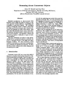
1 Introduction The goal of qualitative reasoning is to draw useful conclusions from incomplete knowledge, particularly for problems where methods relying on numerically precise inputs may be inapplicable. Textbooks, such as Resnick and Halliday's Physics text [17], are an interesting source of problems as they contain both qualitative and numerically-intensive exercises to test the reader's understanding of concepts. The descriptions of the qualitative exercises, including any accompanying diagrams, generally contain very little numerically precise, problem-speci c information and instead seek to cover a large set of scenarios. For example, as in Figure 1, the direction of motion of an object may be given through an arrow in a diagram, but the exact rate of motion may not be given in either the text description of the scenario or the accompanying diagram. This style of problem description is chosen so that the lesson being taught can transfer to many other problems and situations. Qualitative spatial reasoning about the relative position and orientation of

Benjamin Kuipers Department of Computer Sciences University of Texas at Austin Austin, Texas 78712 objects may be required to solve many of these problems.

1.1 Qualitative Spatial Reasoning Several theories have emerged recently for qualitative spatial reasoning about the spatial extent, relative position, and orientation of objects. The work may be roughly divided into two groups: eorts to develop formal, intuitive descriptions independent of any particular device or domain, and eorts to develop methods for modeling and simulating complex mechanisms whose behavior depends on the spatial con guration. Cui, Cohn, and Randell [5], Freksa [7], Galton [8], Mukerjee and Joe [13], Nielsen [14], and Weinberg, Uckun, and Biswas [19], have all been among the contributors of formal, intuitive theories of qualitative spatial reasoning. While these theories have been both simple and elegant, the utility of these approaches for use in larger reasoning systems has yet to be demonstrated. For example, Cui, Cohn, and Randell [5] provide an axiomatic description of the relative positions between objects, but cannot reason explicitly about motion. Their theory allows one to determine all possible spatial states that may follow a given state, but does not include a method for using more speci c information, such as a motion vector, to narrow the possibilities. Faltings, Forbus, Nielsen, Joskowicz, and Sacks [6, 9] address the problem of modeling complex mechanical devices whose behavior depends on the spatial con guration of their mechanically-linked components. Their solutions share the property that a numerically precise description, the con guration space, is computed to provide all possible legal con gurations of the components of the device. The relevant qualitative features are then extracted from this description to reason about the interactions between any moving components. This non-intuitive solution is required, in part, because the problems addressed require reasoning about the exact shapes of objects, a spatial prop-

erty that is dicult to describe in purely qualitative terms. We are developing a new theory for qualitative spatial reasoning which merges a simple, intuitive description of the spatial extent, relative position, and orientation of objects with existing methods for qualitative reasoning about dynamically changing worlds. Our methods are being applied in a problem solver which addresses textbook problems from the magnetic elds domain. The problem solver makes use of the QPC [3] and QSIM [11] qualitative reasoning systems and the Algernon [4] knowledge representation system. This implementation architecture will allow us to inherit additional capabilities as they are developed for the underlying systems, such as methods for incorporating incomplete quantitative knowledge into the reasoning process [12, 10]. This paper describes two implemented modules of this ongoing project. The Figure Understander accepts a diagram and a text description as input, as in Figure 1, and provides an integrated description of the initial spatial and dynamic state of the world. The Motion Understander reasons about motion and its effects on the spatial state. These modules are used by the problem solver to recognize spatial con gurations of importance in the magnetic elds domain. These special con gurations may trigger domain processes which may in turn change the spatial state. Thus, the integration of spatial and dynamic reasoning is an important issue in our work.

2 An Overview of the Problem We shall now present an illustrative example which outlines the issues addressed in this paper. Consider the scenario in Figure 1. We have a conducting loop that is rolling down a ramp into a magnetic eld. The problem statement associated with the diagram asks: \Describe the motion of the loop as it rolls from the top of the ramp to the bottom". Problems of this type may be solved through qualitative simulation.

2.1 Input Description The rst step in automating a solution is to provide a means to describe the problem. The input to our system is similar to that given to the reader of a textbook: We provide spatial information through a graphically drawn diagram and descriptions of dynamic changes through accompanying text, such as the diagram and text given in Figure 1. The Figure Understander module is responsible for extracting the relevant information in each form of input and provid-



Diagram:



Text: The loop is rolling down the ramp.

Figure 1: The diagram and accompanying text description provided as input for a magnetic elds problem.

Figure 2: Diagram in Figure 1 redisplayed within a frame of reference chosen to maximize the number of edges aligned with the coordinate axes. ing an integrated description of the initial spatial and dynamic state of the world. The rst task of Figure Understander is to choose an appropriate global frame of reference for the problem. This task is important since the solutions to magnetic elds problems frequently involve cross product operations on vectors. A useful heuristic that can simplify the vectors involved is: \Maximize the number of object surfaces (edges) and lines that are aligned with the coordinate axes". If a new frame of reference is chosen, the input diagram is automatically rotated (numerically) to t the new frame of reference. All spatial knowledge is then extracted from the rotated diagram. In Figure 2, we show the rotated diagram produced by Figure Understander for the input diagram in Figure 1. The next issue, then, is to correlate the information in the diagram with that in the text description. Diagrams can provide spatial information, but do not contain domain knowledge about the names and prop-

erties of the objects in the scene, or descriptions of dynamic changes that may be taking place. Text can provide domain speci c information and describes dynamic changes, but may contain very little information about the spatial state. The issue of integrating text and diagram input has been addressed in other work [15, 18], but the methods assume that the pictures or diagrams are provided in visual form. They address the classic visual scene analysis problem [2] of deciding which line segments belong together as parts of the same object, and which are only accidentally intersecting. Domain libraries are used to recognize semantically meaningful collections of objects in the diagram. For example, to match the library model of a `pulley', the diagram may need to contain a circular object with two attached lines. In our work, we assume that each closed object (e.g., a polygon) is drawn as a single entity with the use of a graphical editor, and is therefore readily identi able from the output of the editor. We then provide a framework for directly associating graphical objects, based on the shading, patterns, and brush types used, with domain objects. This provides a means for directly matching domain object references in the text with those in the diagram. When there are multiple matches in the diagram for a domain object type given in the text, we can use spatial relations given in the text, such as `the building to my left', to select among the possible matches. These methods are described further in Section 3.

Once the loop fully enters the eld, it becomes enclosed in the eld. Other than motion, no other process is active until the loop reaches the right boundary

2.2 Spatial and Dynamic Reasoning

The Figure Understander is given a diagram, an accompanying text description, and domain knowledge about the world objects, and is asked to produce an integrated knowledge base description that captures the spatial and dynamic state of the world given in the initial scenario. In the current implementation, The idraw graphical editor is used to generate the diagram, and the Algernon knowledge representation language [4] is used to maintain the knowledge base. The rst step in integrating diagram and text input, after choosing a frame of reference for the diagram, is to associate a common semantics with the objects in the diagram and the text. For objects in diagrams, we use shading and patterns to designate particular domain object types. In Figure 1, the white shading is used to designate a loop of wire without any initial current ow, the black shading is used to designate an immobile supporting object, and the dot pattern is used to indicate a magnetic eld directed outward. For text processing, we use a domain speci c semantic interpreter to recognize speci c sentence types and words from the output of an ATN parser. The output of the semantic interpreter is a structure con-

The Motion Understander is responsible for maintaining the spatial state of the world as objects translate and rotate. The spatial state includes a description of the location, relation position, and orientation of all objects. This information can be essential for the problem solving process, as shown by the highlighted phrases in the following explanation for the situation in Figure 2. Phrases describing relative positions are italicized and phrases involving orientation are in typewriter font. In Figure 2, the loop is initially to the left of the eld and is moving to the right. We need to recognize that the next qualitatively interesting state occurs when the loop reaches the left edge of the eld. At that point, the loop begins to overlap the eld. The ux through the loop increases, resulting in an induced emf which causes a clockwise current ow in the loop. A resultant force then acts on the right side of the loop which opposes its movement into the magnetic eld.

of the eld. At that point, the area of overlap begins to decrease, and therefore the ux through the loop decreases. An induced emf is established which in turn causes a counterclockwise current ow in the loop. A resultant force then acts on the left side of the loop which opposes its movement out of the eld. An additional eect is that a new magnetic eld is created while there is current ow in the loop. In this example, the new eld simply opposes the changes in ux through through the loop and plays no other active role. However, in other devices, such as a transformer, magnetic elds dynamically created in this manner play an important role and have to be explicitly included in the model. We are currently addressing the issue of modeling dynamically created spatial objects. Other issues to be addressed include methods for reasoning about torques and rotational motion, which are necessary for modeling such devices as motors and generators. In Section 4, we describe our implemented methods for modeling the spatial extent, relative position, and orientation of two and three dimensional objects, and demonstrate the use of these models in reasoning about translational motion.

3 Figure Understander

taining two parts: a search path into the knowledge base for locating domain objects given in the diagram and a collection of new facts to be added about these objects.

3.1 Picture Semantics The connection between the shading of the objects in the diagram and the domain semantics is given through a picture semantics description, as illustrated in Figure 3. The main properties of the picture semantics description are given below. First, graphical patterns may be associated with domain object types. Under :patterns-for-2d-objects, the solid-white pattern is associated with the domain object type no-current-loop, a conducting loop without any initial current ow. Second, individual object types can be grouped into object classes. Under :object-groups, we include no-current-loops as members of the class conducting-loops. One may also specify naming abbreviations for members of the class. E.g., Conducting loops have a naming abbreviation of `L', so all instances of conducting loops in the diagram will have names L, L1, L2, etc., in the knowledge base. Third, the domain semantics for object classes and individual object types may be speci ed. The semantics are expressed as predicates in the syntax of Algernon. E.g., under :object group semantics, we specify that all diagram objects that have a pattern associated with the set conducting loops are members of the knowledge base set `conducting-loops', that they are conducting objects, that they are mobile, and that they are solid objects.

3.2 Text Processing The text processing task results in a query and assert operation on the knowledge base. The query is of the form \identify objects with certain domain properties", and the assert operation speci es a collection of new facts to be added about the objects. The query may include descriptions of spatial relations which have to be satis ed between the objects of interest. For example, given the speci c domain knowledge that there will always be a vector in the diagram which precisely identi es the direction of motion, when interpreting the text that the `loop' is `rolling', we trigger a query to nd a vector and a loop in the diagram, and then assert that the vector is a velocity and that the direction of motion of the loop is the direction of the vector.

Interpreting text sentence: (THE LOOP IS ROLLING DOWN THE RAMP) The following Algernon path shall be asserted: ((:THE ?V1 (MEMBER CONDUCTING-LOOPS ?V1) (MOBILITY-OF ?V1 MOBILE)) (:THE ?V2 (MEMBER SUPPORT-OBJECTS ?V2)) (:THE ?V3 (MEMBER VECTORS ?V3) (VECTOR-DIRECTION-OF ?V3 S ?VEL-VECT)) (ISA ?V3 VELOCITIES) (VELOCITY-VECTOR ?V1 S-INIT-MODEL ?VEL-VECT) (SURFACE-CONTACT ?V1 ?V2 S-INIT-MODEL))

Figure 4: The Algernon path generated for the text in Figure 1. Figure 4 shows the query and assert path generated for the text in Figure 1. The query seeks to locate three objects: a conducting loop, a supporting object, and a vector. The assert adds the following: the vector is a velocity, the direction of velocity of the loop is equal to the direction of the vector found in the diagram, and that there is contact between some surface of the loop and the supporting object. Note that since certain properties may change over time, we sometimes scope predicates - either to a particular state (s-init-model) or to the entire scenario (s).

4 Motion Understander Motion Understander seeks to maintain the spatial state (i.e., the spatial extent, relation position, and orientation of objects) of a dynamically changing world. Reasoning about the relative positions of objects, such as whether one object is to the left of another, requires knowledge of the region of space occupied by each object (spatial extent), and a frame of reference. For the magnetic elds problem solver, we use the extrinsic frame of reference of the rotated diagram. To represent the region of space occupied by an object, we need to model the shape of the object. In some problems, such as determining whether two gears will mesh together [6], exact shapes play a very important role. For other problems, it is more important to reason about the eects of possible changes in spatial state, and the exact shapes of objects are not of great concern. For this latter category of problems, an abstraction can be introduced for the shape of an object to simplify the reasoning process.

(defpict pictures-for-mag-fields ; IDRAW pattern :patterns-for-2d-objects ((light-rect-mesh (solid-black (solid-white

; USER Domain Object field-out-of-page) other-object) no-current-loop))

; Object Class Abb. Name ((conducting-loops L

:object-groups

Class Members (no-current-loop)))

; Class Name ((conducting-loops ; Semantics Expressed as Algernon Predicates. ((member conducting-loops ?obj) (is-conducting-object ?obj TRUE) (mobility-of ?obj mobile) (is-solid ?obj TRUE)))))

:object-group-semantics

Figure 3: Example of a partial picture semantics for the magnetic elds domain. tm(a) tm(b) − V1 E1

rm(b)

lm(a)

V2

bm(a)

bm(b) V3

A

B

A: Bounding Circle B: Rectangular Bounding Box

Figure 5: Examples of bounding boxes and bounding circles for two polygons.

4.1 Bounding Cubes and Bounding Spheres as Abstractions of Shape We use two types of abstractions, a rectangular bounding box and a bounding circle [16], to ap-

proximate the region occupied by an object. For problems in three-dimensional space, these can be replaced by a bounding cube and a bounding sphere respectively. In Figure 5, we illustrate our abstraction method on two polygons. We draw a bounding circle around object A and a rectangular bounding box around object B. We use the bounding box approximation for problems where objects may translate, but not rotate, and

the bounding circle for problems where objects may both translate and rotate. The two abstractions are necessary to guarantee that the actual region of space occupied by an object is contained within the region of space de ned by the abstraction used. Abella and Kender [1] describe a shape abstraction method based on rectangular bounding boxes that does not provide this guarantee. Thus, in their approach, it is possible to conclude, for example, that two objects are not `near' each other when they are actually intersecting! To illustrate why rectangular bounding boxes are insucient for modeling rotating objects, consider object A in Figure 5. The bounding box for this object exactly covers the region occupied by the object. Any rotation in the X-Y plane would involve crossing the borders of the bounding box. The weaker abstraction, a bounding circle centered at the center of gravity of the enclosed object, can be used to ensure that the enclosed object will remain fully contained within the circle at all times.

4.2 Modeling Spatial Extent Rectangular bounding boxes and bounding circles are powerful abstractions for qualitative spatial reasoning because numerically precise information is not required, even in a dynamically changing world, to maintain a description of the bounding boxes and bounding circles. Our bounding box and bounding circle approximations describe the spatial extent (absolute position) of an object qualitatively in terms of an object's extremal points: the topmost (tm), rightmost (rm), bottommost (bm), and leftmost (lm) points. To rea-

son about three dimensional objects, we may add two more extremal points: the frontmost and rearmost points. We may use knowledge of the direction of motion of objects to determine changes in the values of the four or six extremal points and thus maintain an understanding of the location and extent of the object. For the remainder of this discussion, we shall deal with two-dimensional objects in X-Y plane. The bounding box approximation draws the box around the actual extremal points of the object, and it's possible that an edge forms an extremal point. In Figure 5, object A has four extremal edges, and therefore, the bounding box approximation exactly matches the actual perimeter of A. The bounding circle approximation uses the maximumvalue obtained for each extremal point if the object is allowed to rotate about its center of gravity. The radius of the bounding circle is given by the maximum distance from the center of gravity of the object to any point on the perimeter. In Figure 5, we show the bounding circle for object A. Notice that the extremal points of the bounding circle are dierent from the actual extremal points of the underlying square object.

4.4 Relative Positions and Translational Motion

4.3 Modeling Orientation

Our representational framework precisely ts several existing systems for dynamic qualitative reasoning. In particular, we make use of the QPC [3] and QSIM [11] systems. We de ne spatial relations of interest through view descriptions in QPC, and use that system to perform the necessary inequality reasoning to determine the current spatial state of the world and to determine how the spatial state changes over time. Because QPC view descriptions are modular structures, a library of important spatial relations may be built incrementally and hierarchically. Figure 6 shows the QPC view descriptions (model fragments) for motion in the X direction and for the spatial relation `left-of'. Under :individuals, we declare what types of objects must be present. Under :operating-conditions, we outline the dynamically changeable inequality conditions that have to be satis ed for the view to be instantiated. Under :relations, we de ne the dynamic eects of the view. For example, X-motion is active for any mobile object whose x-velocity is non-zero. Under :relations, we include the derivative relationship between the xvelocity of the object and the values of its rightmost and leftmost points. In Figure 2, the conducting loop initially has a xvelocity that is greater than zero, and X-motion will be active. Further, since the condition rm(loop) > lm(field) is not true, QPC will instantiate the view left-of(loop, eld). However, QPC recognizes that this condition will eventually be violated, since, as a result

For convex objects, our representation of position based on extremal points also gives the orientation with respect to a global Cartesian frame of reference. We de ne the orientation of a surface of an object through the surface normal direction of that surface. The surface normal direction is given through a triple (X,Y,Z), which represents the X, Y, and Z components of the surface normal vector. Each component can be zero (0), positive (1), or negative (-1). Thus, for a convex, two dimensional object in the X-Y plane, if an edge forms an extremal point, then the orientation of that edge will be (1 0 0) for the rightmost point, (0 1 0) for the topmost point, (-1 0 0) for the leftmost point, and (0 -1 0) for the bottommost point. In addition,  For any surface which lies between the topmost and rightmost points, the orientation vector is (1 1 0).  For any surface which lies between the rightmost and bottommost points, the orientation vector is (1 -1 0).  For any surface which lies between the bottommost and leftmost points, the orientation vector is (-1 -1 0).  For any surface which lies between the leftmost and topmost points, the orientation vector is (-1 1 0).

We model spatial relations between pairs of objects (relative positions) through inequality relations on their extremal points [16]. For the objects in Figure 5, the inequality relation rm(A) < lm(B), represents the fact that A is to the left of B. These inequality relations also provide the additional information that a qualitatively interesting state will occur when the relations change (e.g., when lm(A) = rm(B)). This can be used to study the eects of translational motion on the spatial state. For example, the values of the rightmost and leftmost points of an object will change over time if the X-velocity of the object is non-zero. In Figure 5, if the X-velocity of object A is positive, the coordinate value of its rightmost point will increase over time, and we can recognize that a qualitatively interesting state will occur once rm(A) = lm(B).

4.5 Integration with Existing Systems for Qualitative Modeling and Simulation

(defview X-motion () :individuals ((obj :type mobile-objects)) :operating-conditions ((not (q= (x-velocity obj) ZERO))) :relations ((d/dt (rm-xval obj) (x-velocity obj)) (d/dt (lm-xval obj) (x-velocity obj)))) (defview Left-of () :individuals ((left-obj :type world-objects) (right-obj :type world-objects)) :operating-conditions ((not (q> (rm-xval left-obj) (lm-xval right-obj)))))

MAX

. .. . ..↑ .. . ..↑.↑. . . . . .↑ .. . ..↑.↑. . . . . .↑ .. . ..↑.↑. . . . . .↑ .. . ..↑ ↑ .. . ..↑ .. . ..↑.↑

. .. . ..↑ .. . ..↑.↑. . . . . .↑ .. . ..↑.↑. . . . . .↑ .. . ..↑.↑. . . . . .↑ ↑ .. . ..↑ .. . ..↑.↑

T0

T1

T2

T3

T4

T5

L.LM-XVAL

↑

...

T0

. .↑ .. . ..↑.°. . . . . .° .. . ..°.↓. . . . . .↓ . . . .

.↓

T2

T3

T4

T5

INF

° .. . ..° .. . ..°... ° . . . . .° .. . ..°... ° . . . . .° .. . ..°

0

T1

T2

T3

T4

T5

0

↑

...

MINF T0

T1

T2

T3

T4

T5

L.AREA-OF-OVERLAP-DERIV

. .↑ .. . ..↑.°. . . . . .° .. . ..°.↓. . . . . .↓ . . . .

INF

.↓

INF

° .. . ..° .. . ..°... ° . . . . .° .. . ..°... ° . . . . .° .. . ..°

0

0

MINF T0

T1

T2

T3

T4

T5

L.FLUX-THROUGH-LOOP

MINF T0

T1

T2

T3

T4

INF

° .. . ..° .. . ..°

INF

° . . . . .° .. . ..°

° .. . ..° .. . ..°

° . . . . .° .. . ..°

T1

T3

0 T1

T2

T3

↓ .. . ..↓ . . .

T4

T5

↓↓ . . .

0 T0

T2

T4

. .. . ..↓ . . ↓ .. . ..↓ .. . ..↓.↓ .

. . .. . .. .. . . . . . .. . .. .. . . . . . .. . .. .. . . . . . .. . .. 0 ↓ ↓↓ ↓ ↓↓ ↓ ↓↓ ↓ ↓

INF

. . ..

↓↓ . . .

. . .. . .. .. . . . . . .. . .. .. . . . . . .. . .. 0 ↓ ↓↓ ↓ ↓↓ ↓ ↓

MINF T1

T2

T3

T4

T5

DIF-- . .. . ..↓ .. . ..↓.↓. . . . . .↓ . . ↓ .. . ..↓ .. . ..↓.↓ .

INF

. . ..

↓↓ . . .

MINF T0

T1

T2

T3

T4

T1

T2

T3

. .. . ..↓ .. . ..↓.↓. . . . . .↓ .. . ..↓.↓. . . . . .↓ . . ↓ .. . ..↓ .. . ..↓.↓ .

. . .. . .. .. . . . . . .. . .. 0 ↓ ↓↓ ↓ ↓ T4

T5

T5

DIF-- INF

. . ..

↓↓ . . .

MINF T0

T5

L.LOOP-CURRENT-FLOW INF

. . ..

T5

L.FLUX-THROUGH-LOOP-DERIV

DIF--

Figure 7 shows the qualitative behavior produced by Motion Understander for the example in Figure 2. The loop starts to the left of the eld, and is moving to the right. The values of the rightmost and leftmost points of the loop (L.RM-XVAL, L.LM-XVAL) are steadily increasing. After some time, the loop begins to move into the eld, and the area of overlap increases. Once the loop is fully enclosed in the eld, the area of overlap remains constant until the loop begins to exit the eld to the right, when it decreases to zero. The ux through the loop changes with the area of overlap. This change results in an induced emf being set up in the loop which in turn causes a current ow in the loop. We are currently expanding our implementation of the magnetic elds domain theory to reason about magnetic forces and their eects. The variables whose names begin with `DIF' are QPC generated variables which encode the inequality relationships of interest in the simulation. Notice that the qualitatively interesting changes occur whenever one of the `DIF' terms crosses zero. For example, when the variable DIF-- is positive, the loop is to the left of the eld. The value becomes zero at the instant when the loop and the eld meet.

T1

L.RM-XVAL

L.AREA-OF-OVERLAP

T0

4.5.1 The Qualitative Behavior for the Example in Figure 2

0 T0

INF

L.INDUCED-EMF-MAG

of X-motion being active, the coordinate value of the rightmost point of the loop will increase and become equal to the leftmost point of the eld.

. .↑ MAX

MINF

T0

Figure 6: Examples of QPC view descriptions: Xmotion and Left-of.

...

0

. . .. . .. 0 ↓ ↓ MINF

T0

T1

T2

T3

T4

T5

DIF--

Figure 7: Qualitative behavior produced by Motion Understander for the example in Figure 2. The derivative of the area of overlap is constant while the conducting loop is entering and exiting the magnetic eld due to the use of the rectangular bounding box abstraction for the circular conducting loop.

5 Summary and Future Work We have described two modules of an ongoing project to develop methods for qualitative spatial reasoning which are intuitive and yet powerful enough to reason about problems in a dynamically changing world. Figure Understander accepts a diagram and a text description as input and integrates the unique information in each within a single knowledge base. Motion Understander maintains an understanding of the spatial state in a dynamically changing world. We described an implemented method for reasoning about changes in the global spatial state under translational motion. Two abstraction of shape, bounding cubes and bounding spheres, were introduced to approximate the spatial extent of objects. These abstractions were shown to be use useful for studying changes in relative position as objects move about in the world. The remaining work will cover rotational motion.

An important eect of rotation is that it can change the orientation of an object with respect to a global frame of reference. In Physics, orientation information can be very important when a problem requires knowledge of exactly where a force acts on an object. For example, a force whose line of action does not cross the center of gravity of the object will cause a torque, which in turn may cause the object to rotate. To solve these problems, we are developing methods for modeling orientation as a local property of individual objects. These models will supplement the methods for describing the global spatial state that were described in this paper.

Acknowledgements We would like to thank Richard Mallory and James Lester for providing helpful comments. This research was supported in part by NSF grants IRI-8904454, IRI-9017047, and IRI-9216584, and by NASA contracts NCC 2-760 and NAG 9-665.

References [1] A. Abella and J. Kender. Qualitatively describing objects using spatial prepositions. In Proc. 11th National Conf. on Arti cial Intelligence, Cambridge, MA, 1993. AAAI/MIT Press. [2] D. H. Ballard and C. M. Brown. Computer Vision. Prentice-Hall, Englewood Clis, NJ, 1982. [3] J. Crawford, A. Farquhar, and B. Kuipers. QPC: A compiler from physical models into qualitative dierential equations. In Proc. 8th National Conf. on Arti cial Intelligence, San Mateo, Calif., 1990. Morgan Kaufmann. [4] J. Crawford and B. Kuipers. Algernon - a tractable system for knowledge-representation. In AAAI Spring Symposium on Implemented Knowledge Representation and Reasoning Systems, Palo Alto, CA, 1991.

[5] Z. Cui, A. G. Cohn, and D. Randell. Qualitative simulation based on a logical formalism of space and time. In Proc. 10th National Conf. on Arti cial Intelligence, Cambridge, MA, 1992. AAAI/MIT Press. [6] K. Forbus, P. Nielsen, and B. Faltings. Qualitative spatial reasoning: The clock project. Arti cial Intelligence, 51:417{471, 1991. [7] C. Freksa. Using orientation information for qualitative spatial reasoning. In A. Frank, I. Campari,

and U. Formentini, editors, Theories and Methods of Spatio-Temporal Reasoning in Geographic Space. Springer-Verlag, Berlin, 1992.

[8] A Galton. Towards an integrated logic of space, time, and motion. In Proc. 13th Int. Joint Conf. on Arti cial Intelligence, San Mateo, Calif., 1993. Morgan Kaufmann. [9] L. Joskowicz and E. Sacks. Computational kinematics. Arti cial Intelligence, 51:381{416, 1991. [10] H. Kay and B. Kuipers. Numerical behavior envelopes for qualitative models. In Proc. 11th National Conf. on Arti cial Intelligence, pages 606{ 613, Cambridge, MA, 1993. AAAI/MIT Press. [11] B. Kuipers. Qualitative simulation. Arti cial Intelligence, 29:289{338, 1986. [12] B. Kuipers and D. Berleant. Using incomplete quantitative knowledge in qualitative reasoning. Proc. 7th National Conf. on Arti cial Intelligence, 1988.

[13] A. Mukerjee and G. Joe. A qualitative model for space. In Proc. 8th National Conf. on Arti cial Intelligence, Cambridge, MA, 1990. AAAI/MIT Press. [14] P. Nielsen. A qualitative approach to mechanical constraint. In Proc. 7th National Conf. on Arti cial Intelligence, San Mateo, Calif., 1988. Morgan Kaufmann. [15] G. Novak and W. Bulko. Diagrams and text as computer input. Journal of Visual Languages and Computing, 4:161{175, 1993. [16] R. Rajagopalan. A model of spatial position based on extremal points. In Proceedings of the ACM Workshop on Advances in Geographic Information Systems, Arlington, VA, November

1993. [17] J. Resnick and D. Halliday. Fundamentals of Physics. John Wiley and Sons, New York, third edition, 1988. [18] R. Srihari. Piction: A system that uses captions to label human faces in newspaper photographs. In Proc. 9th National Conf. on Arti cial Intelligence, Cambridge, MA, 1991. AAAI/MIT Press. [19] J. Weinberg, S. Uckun, G. Biswas, and S. Manganaris. Qualitative vector algebra. In Boi Faltings and Peter Struss, editors, Recent Advances in Qualitative Physics. MIT Press, Cambridge, MA, 1992.