Quality indices for (practical) clustering evaluation Margarida G.M.S. Cardoso1 Department of Quantitative Methods, ISCTE Business School, Av. das Forças Armadas, 1649-026, Lisboa, Portugal E-mail:
[email protected] 1
corresponding author
André Ponce de Leon F. de Carvalho Department of Computer Science Institute of Mathematics and Computer Science University of São Paulo, Av. Trabalhador Sãocarlense, 400, CEP 13560-970, São Carlos, SP, Brazil E-mail: andré@icmc.usp.br
Abstract Clustering quality or validation indices allow the evaluation of the quality of clustering in order to support the selection of a specific partition or clustering structure in its natural unsupervised environment, where the real solution is unknown or not available. In this paper, we investigate the use of quality indices mostly based on the concepts of clusters’ compactness and separation, for the evaluation of clustering results (partitions in particular). This work intends to offer a general perspective regarding the appropriate use of quality indices for the purpose of clustering evaluation. After presenting some commonly used indices, as well as indices recently proposed in the literature, key issues regarding the practical use of quality indices are addressed. A general methodological approach is presented which considers the identification of appropriate indices thresholds. This general approach is compared with the simple use of quality indices for evaluating a clustering solution. Key words: cluster validation, validation indices, quality indices, clustering.
1
1
Introduction
Cluster Analysis is a process designed to discover (or uncover) clusters of objects from a data set. Ideally, the objects in each cluster should share a significant number of characteristics with other objects in the same cluster and differ from objects belonging to other clusters. Partitions constitute the more popular clustering structure and are useful for several applications. Since Cluster analysis is a very practical subject (as stated by [24] in the first sentence of their book), the present work is focused on the practical evaluation of partitions. The main clustering evaluation criterion should concern the degree of fit between the partition obtained (derived through cluster analysis) and the real or true partition. However, since the real partition is unknown, the clustering evaluation surrogate’s issue is the identification of a good enough partition. Although several quality indices have been proposed and analyzed in the literature, and even some works have compared the advantages and disadvantages of several quality indices, this paper contributes to the advance of research in this area by highlighting some important issues regarding the use of these indices in practical problems. It also proposes a general methodology – the generalization of a Monte Carlo based approach for virtually all quality indices – to support the identification of homogeneity thresholds for quality indices, which is the main contribution. The following sections describe contributions from the literature dedicated to clustering evaluation (partitions, in particular) and the use of quality indices. The first section addresses homogeneity tests, which can be used to identify when there is no clustering structure. The second section covers a group of quality indices concerned with the measurement of clusters’ compactness and separation. The third section focuses on current work and addresses important issues related with the practical use of quality indices. It proposes a general methodological approach for clustering evaluation using quality indices. Section 4 presents experimental results obtained with the use of the proposed methodology.
In the end, some conclusions and
perspectives are presented. In order to support the presentation of the main issues of this paper in the following sections, the basic notation is established in advance:
2
Π
Partition
ΠK
Partition with K clusters
C1,…CK
Set of K clusters of a partition
D = [d(xi,xj)]
Matrix of (original) distances between objects
ˆ = [dˆ( x i , x j )] D
Matrix of estimated distances (derived from clustering results) between objects Between clusters distance measure (it can refer to either a partition ΠK or
B
to a specific pair of clusters) Within clusters distance measure (it can refer to either a partition ΠK or
W
to a specific cluster) K*
The best number of clusters
x1, …, xN
Objects to be clustered
2
Homogeneity tests
Before performing the cluster analysis, it is important to decide if it is worthwhile, i.e. the data might be sampled from a homogeneous population without any clustering structure. That is the perspective underlying the homogeneity hypothesis testing approach. The null hypothesis, H0, usually employed in homogeneity tests, should translate the fact that the data originate from a population where no clustering structure exists. There are some null hypothesis which are commonly used to translate the absence of a structure (see [18] or [5]): -
Uniform Model, which assumes that objects can be represented by points uniformly distributed in a region A from a J-dimensional space.
3
-
Unimodal Model, where the joint distribution of the clustering base variables is supposed to have the same unimodal density (e.g. multivariate normal with unknown mean (µ) and covariance matrix σI)
The Uniform Model is sensitive to the region A definition. This region A may be either the unit Jdimensional hipercube or hipersphere (assuming that data are standardized) or may be specified taking the observed data values into consideration (e.g. A may be the convex hull of the points in the data set). This latter definition may allow the construction of tests which are less influenced by unimportant differences between the model and data, but it may imply heavy demands on computational resources (e.g. unless J is small, it is hard to determine the convex hull of the points in the data set) [5]. In the Unimodal Model, the null hypothesis can also take the data into consideration, by specifying a data-influenced covariance matrix. In addition to defining the homogeneity H0 hypothesis, a suitable heterogeneity H1 hypothesis must be characterized. The most general H1 (referring to pure homogeneity tests) does not include any information concerning the clustering structure (not even the number of clusters). These homogeneity tests configure the first (preliminary) step in the clustering evaluation process. In order to test a specific null hypothesis H0 against an alternative hypothesis H1, an appropriate test statistic (TS) must be adopted and its distribution under H0 must be determined. Depending on the specified hypothesis, one can consider different alternatives for the TS. e.g. the largest nearest neighbour distance within the set of entities can be considered to test the Uniform Model [4]. In most cases, it is not possible to derive the homogeneity TS’s exact distribution. To overcome this limitation, one can, sometimes, recur to asymptotical distributions.
As an alternative
approach, Monte Carlo simulation procedures can be used to generate samples under the homogeneity null hypothesis H0 (see Figure 1). This type of procedure enables the construction of a TS empirical distribution, its main drawback being the additional computational cost. (insert Figure 1 about here)
4
In addition to pure homogeneity tests, alternative formulations have been proposed. One of them, the Random Label hypothesis [23], takes into account a specific partition to deal with and evaluate. It assumes (null model) that all permutations of the entities’ labels (resulting from cluster assignments) are equally likely. Homogeneity tests are typically referred to quantitative clustering base variables randomly sampled from a population. This is not the case in many practical applications. (Everitt, 2001) makes the following comments on homogeneity tests for practical applications: such tests are not
usually employed in practical applications of clustering. This may be because the available tests are of limited usefulness (p. 180). [27] also comment on the homogeneity tests’ drawbacks: the power of many such statistical tests decreases quickly with increasing data dimensionality. Also, a rejection of null hypothesis does not shed any light on which clustering algorithm to use (p. 2). Despite these drawbacks, homogeneity tests may have a role in the clustering evaluation process, which will be discussed in the paper.
3
Quality indices
Once having established that there is a real clustering structure (whether the conclusion relies on theoretical or empirical and practical grounds), one specific clustering solution may be derived and evaluated. A commonly used measure for evaluating the quality of a clustering solution is the Hubert’s Γ statistic (e.g. [23]), which measures the fit between the partition and the clustering base data:
(
)
ˆ = Γ D, D
n −1 n 2 ∑ ∑ d(x i , x j )dˆ(x i , x j ) n (n − 1) i =1 j=i+1
(1)
where n is the number of objects and dˆ (x i , x j ) = 1 if the objects xi and xj belong to the same cluster or 0, otherwise. Hence, it can be thought as a point biserial correlation between the original distance matrix (e.g squared Euclidean distance) and the matrix of estimated distances (part of the clustering results). Alternatively, the estimated distance dˆ between two objects,
which can be derived from the clustering solution, may be quantified as the distance between points (typically centroids) representing the clusters to which the two objects belong.
5
The Hubert’s Γ statistic can be normalized, yielding a correlation measure between the original and the estimated (through clustering) distances, its maximum and minimum value being 1 and −1, respectively:
Γnorm
(
)
n −1 n 2 ˆ = D, D ∑ ∑ n (n − 1) i =1 j=i +1
[d(x , x ) − d ]dˆ(x , x ) − dˆ i
j
i
j
s d s dˆ
(2)
Where sd and s dˆ refer to the empirical standard deviation of d and dˆ , respectively.
Larger Hubert’s Γ statistic values indicate good fitness between the data and the clusters. Larger values also denote compact clusters, meaning that the objects inside a cluster are close to its representative point. There are some desirable properties of clustering structures, related to distinguishing partitions’ qualities, which make them unusual or valid. One of them is compactness. In fact, many authors say that the compactness, and also separation properties, of a clustering structure define its quality. Several works try to measure these properties by the homogeneity-within and heterogeneity-between clusters (e.g. [10]). Thus, compactness measures the internal cohesion among objects within clusters and separation measures the isolation of clusters when compared to other clusters. While this general idea is frequently accepted, many definitions of compactness and separation have been proposed, originating different quality indices to measure the quality of a clustering structure. Several indices are described in [19], for example. Examples of indices are presented on Table 1. They are generally based on some compactness (within clusters) to separation (between clusters) measures’ ratio. (Insert table 1 about here) The Dunn index [14] measures the between-within distances ratio. The best partitions should exhibit the largest index values corresponding to compact and well separated clusters:
6
( )
dunn Π K =
min min B(C k , C k ' ) k
k '≠ k
(3)
max W (C k )
k∈{1... K }
Originally, B(C k , C k ' ) =
(
d x ,x min d (x, x ') and W (C k ) = max 1 2
x∈C k ; x '∈C k '
x x ∈C k
1
2
)
The Calinski and Harabask index [10] is a pseudo-F-statistic, which also measures the betweenwithin distances ratio: B(Π K ) (K − 1) CH (Π ) = W (Π K ) (n − K ) K
(4)
In experiments performed by [29], the CH index was the best among 30 alternative criteria evaluated to determine the best clustering structure (/best number of clusters). [11] rearranged the within-between distances in the following index, where the best values should be the lowest possible: dav − bould(Π K ) =
W (C k ) + W (C k ' ) 1 K max ∑ K k =1 k '≠ k B(C k , C k ' )
(5)
The Silhouette width measure was proposed by [38] as a graphical aid to the interpretation and validation of cluster analysis. It measures the difference between separation and compactness for each observation xi inside a cluster Ck: silh( x i ; C k ) =
b( x i ; C k ) − w( x i ; C k ) max{b( x i ; C k ), w( x i ; C k )}
(6)
where b( x i ; C k ) = min k '≠ k
∑
j∈C k '
d (x i , x j ) # Ck '
measures the average distance to elements of the nearest cluster
and w (x i ; C k ) =
d(x , x ) ∑{ } # C − 1 measures the average distance to elements of the same cluster. i
j∈C k − i
j
k
7
The average Silhouette index aggregates Silhouette widths from all observations in the corresponding clusters. It can be used to help evaluating a clustering structure [24]:
( )
av − silh Π K =
1 K ∑ silh(C k ) K k =1
(7)
where silh (C k ) =
1 # Ck
∑ silh(x ; C ) i
k
i∈C k
A good partition should then exhibit a high average Silhouette index. Another (recent) example is the PBM index [34]:
( ) ( )
( )
1 W Π1 = max B(C k , C k ' ) K k ,k ' K W Π
( )
1 = K
PBM Π
K
2
(8)
more specifically,
PBM Π
K
(
)
d xi , x ∑ k k' i =1 max d x , x K n k ,k ' k z ik d x i , x ∑∑ k =1 i =1 n
(
)
(
)
2
(9)
where zik=1 if i ∈ Ck and 0, otherwise. The second factor of PBM increases as K increases (since the denominator’s within-clusters distance decreases as K increases). Therefore, it encourages the formation of more compact clusters. The third factor also increases with K. It favours separation between pairs of clusters. The authors of PBM point out that the use of the maximum pairwise inter-cluster distances instead of using a minimum, a sum, or an average, presents some advantages related to the way this function behaves when K increases, the maximum PBM indicating the best partition (number of clusters). According to previous experimental results, this index presents a good performance when compared to the Dunn index or to the Davies-Bouldin index [34].
8
Some indices were originally proposed as a stop criterion for a clustering procedure, indicating whether the number of clusters is adequate (e.g the Davies-Bouldin index, [11]). Nevertheless, they all measure the goodness of partitions and can be employed for the more general purpose of evaluating several candidate partitions. It is, however, possible to incorporate in an index’s formula the within-clusters and between-clusters distances for the comparison of different numbers of clusters. This is the case of the Hartigan index [20]. The Hartigan index explicitly compares within-clusters distances for partitions with K and K+1 clusters, in order to decide whether to include (or not) a new cluster in a partition with K clusters:
( )
Hartigan Π K
K W (C k ) ∑ 1 Kk +=11 = − 1 n − K −1 W (C k '' ) ∑ k ´=1
(10)
It is worthwhile to note that the partition ∏K+1 is not necessarily obtained by splitting one of the clusters in ∏K+1 and, therefore, the Hartigan’s mean square ratio is conceivably negative. It should also be noted that each index looks for a different structure in the data and that the choice of a particular index is generally influenced by the user prior knowledge. The referred list of indices (Table 1) is not at all exhaustive. There are many quality indices and new indices are still being proposed. Nevertheless, this list includes some of the most popular indices (for crisp clustering evaluation), as well as some recent quality indices. More importantly, it enables the comprehension of general clustering evaluation quality indices relying on the properties of compactness and separation. In any case, the reader may always refer to other works, including additional index proposals (e.g. [29] and [33] more recent). Finally, it is worthwhile to note that some of the previously mentioned quality indices have been generalized to clustering structures other than partitions. For example, extended versions of the Dunn index or the PBM indices can be used to evaluate fuzzy clustering structures, as can be seen in ([3] and [34], respectively. In addition, there are also alternative indices that specifically address the quality of fuzzy partitions (e. g. [25], [7] or [43]).
9
4
Practical issues when using quality indices
4.1
Quality indices relative thresholds
Understanding and put in practice the concept of good partition is not an easy task (e.g. [28]). As previously stated, several quality indices (QI) have been proposed to support the selection of a good partition among a set of candidate partitions (yielded by different numbers of clusters or alternative parameterizations of a clustering algorithm, for example). Although some indices have clearly defined maximum and minimum values, it is difficult to define which indices values indicate an adequate partition. In fact, it is easy to propose indices of cluster validity. It is very difficult to fix thresholds on such indices that define when the index is large or small enough to be “unusual” or valid [23] (p. 144). The most commonly used strategy to address this threshold problem is to provide comparisons between several indices values associated with different partitions in order to select the best index value (/partition). Therefore, on practical applications, typically, one can implement a (general) procedure, like the one presented in Figure 2, to support the selection of an appropriate partition among several candidates. These candidates may be originated by minor changes in the clustering procedure, which may range from alternative algorithm parameters to different sets of clustering base variables or numbers of clusters considered. (insert figure 2 about here) Several variants of the soft procedure in Figure 2 can be adopted. When focusing, specifically on selection among partitions with alternative numbers of clusters, this procedure is usually repeated until reaching a maximum number of clusters (Kmax), which must be specified in advance. According to a commonly accepted empirical rule, Kmax should not exceed √n ( [35] cited in [34]). This soft procedure’s focus relies on the appropriate definition of argbest(QI). This definition is usually formulated by establishing empirical (soft) rules dealing with the trade-off between quality (expressed by the QI value) and complexity (number of clusters in particular). This tradeoff may be illustrated by an elbow in a curve picturing the increasing or decreasing index trend, which can be associated with the increasing number of clusters.
10
However, it is worthwhile to note that the indices values may vary with several other factors, such as, the number of observations, the number of clustering base variables and the separation between clusters. An alternative approach is to rely on previous indicators (derived from empirical studies), concerning specific thresholds’ values for specific indices. For example, [20] suggests a crude rule of thumb (p. 91) – hartigan(ΠK) > 10 – that may justify increasing partition size (from K to K+1 clusters). [24] refer to experience with the Silhouette index which has led us to a rather subjective interpretation summarized in (p.88) (Table 2). (insert table 2 about here) Additional clustering evaluation procedures may rely on results from several quality indices, trying to overcome the weaknesses of specific indices by combining their strengths. [6] point out the need for standardization when comparing indices values corresponding to alternative B and W distance measures, for K fixed. They suggest using standardized index versions, based on overall average index values and the corresponding standard deviations:
Std _ ind =
index − average(index ) stdev(index )
(11)
In particular, they use Dunn and Davies-Bouldin indices variants, which are built using several B and W measures. [6] also suggest converting the normalized indices values using weighted voting (minimum weight=1, 2, 3,…, maximum weight=Kmax-1): the advantage of a weighted voting approach lies in a robust aggregation of multiple validation methods in order to improve the estimation of the most adequate clustering partition (p. 832).
4.2
Homogeneity based thresholds for quality indices
Instead of using an empirical (soft) approach to address the threshold problem, an alternative (hard) approach can be considered, which relies on establishing the indices distributions under some null homogeneity hypothesis (H0). This procedure (see Figure 3) enables good choices concerning the observed quality index values, which can be established as significantly apart 11
from this hypothesis. Needless to say that that this approach should rely on random samples of observations, typically drawn from continuous clustering base variables. For example, when using the Hubert’s Γ statistic to evaluate the goodness of fit between data and the clustering structure, the analyst is confronted with the problem of determining Hubert’s Γ critical values for establishing a frontier between good enough partitions and unacceptable ones. The threshold problem related to the Hubert’s Γ statistic is addressed by [23], using the Random Label null model, H0. Under this H0, all permutations of the clustering labels are equally likely
(meaning that clustering labels which yield dˆ (x i , x j ) are imputed at random). The distribution of the Hubert’s Γ statistic under this null hypothesis can be (exactly) calculated when n (the number of objects) is small (all permutations can be easily identified and used in the calculus). When n is large enough, a normal distribution can be considered as an approximation (although the asymptotic normality may not always be appropriate, as stated by [39]). For large (but not enough) n, an alternative approach is suggested by [23], which consider a subset of permutations to approximate the distribution of Γ under H0. Having derived the distribution of the Hubert’s Γ statistic under the Random Label hypothesis, a critical/ threshold value can be determined (for a specific level of significance) that decides upon rejection of H0 (when the observed Hubert’s Γ statistic indicates a good enough partition). Ideally, when using the hard approach to deal with the threshold problem, one should be able to establish one index exact distribution. Since this is most of the times an unattainable (too hard) objective, the more common approach (still hard) is to derive empirical distributions for the index, based on samples’ generation of clustering base variable values, under some specified null homogeneity hypothesis (see Figure 3). Key issues concerning this type of approach are: the definition of adequate null homogeneity hypothesis and the computational cost associated with implementing the Monte Carlo simulation process.
(insert figure 3 about here)
12
An important contribution regarding QI’s construction explicitly dealing with the threshold problem is due to [42]. They propose the use of the Gap statistic for the evaluation of alternative
partitions. They specifically use it to determine an appropriate number of clusters (model order selection). The Gap statistic is based on a measure of within-clusters distance W (Π K ) = ∑ K
1 ∑ ∑ d(x i , x j ) k =1 2# G k i∈G k j∈G k
(12)
In order to determine how much within-clusters distance is too much, [42] use M samples generated under a null homogeneity hypothesis and perform cluster analysis in each. Next, they evaluate the difference (gap) between the obtained average (from M samples) within-clusters distance and the observed one:
( )
gap Π K =
( )
( )
1 M log Wm Π K − log W Π K ∑ M m=1
(13)
The null distribution may be the uniform distribution on the smallest hyper-rectangle that contains the original data. Alternatively it can also be based on the principal components. The threshold value considered for each k is simply the average of the within-clusters distances corresponding to the M samples generated under the null hypothesis (in practice M=20 experiments can be conducted). In order to select the best number of clusters, the procedure may be implemented for k = 1...Kmax (alternative numbers of clusters to consider in the partition). The larger the Gap value, the better the partition. Thus, the partition with the maximum Gap value is selected (corresponding to an adequate number of clusters K*). The authors point out the fact that the Gap statistic has the capacity to recognize the homogeneity situation (when K*=1), as opposed to most alternative indices. In fact, as illustrated in the next section, this (hard) approach (as used in the Gap statistic) can be virtually extended to all quality indices employed for evaluating a clustering structure. In the present paper, this approach is specifically focused on classification data with numerical attributes, which can be considered as normally, distributed (under the homogeneity hypothesis).
13
However, a similar approach can be considered using alternative distributions for the clustering base attributes (e.g. using a uniform distribution for qualitative attributes).
5
Experimental results
In order to illustrate the performance of the soft and hard approaches in the evaluation of clustering structures (see Figure 2 and Figure 3), six data sets are considered: Iris, Wine, Haberman, Diabetes, Breast Cancer and Glass [2]. The analysis resorts to a specific index – the Calinski and Harabask (CH) index – used as an example.
( )= ∑ ∑∑ (x K
CH (Π K
J
) n−K K −1 −x )
∑∑ n k x j − x j k
k =1 j=1 K
J
k =1 i∈C k j=1
ij
2
k 2 j
(14)
Three clustering structures, derived by three alternative clustering methods – the estimation of a Mixture Model (MM) followed by modal allocation, the K-Means (KM) algorithm and the Ward (WA) hierarchical algorithm – are obtained and compared. Under the homogeneity hypothesis (H0), the clustering base variables are assumed to be drawn from Normal populations with parameters corresponding to the average and standard deviation observed in the original samples (see Table 3). For example, the Iris petal length is assumed to follow a N(3.76; 1.76) distribution for any random sample generated under the null homogeneity hypothesis. Twenty random samples are generated according to this procedure for each data set considered. (insert table 3 about here) Since the number of clusters is known in advance it is a priori specified. However, the MM approach could have provided means to decide upon this number for both data sets. The BIC– Bayesian Information Criterion, [16], AIC–Akaike’s Information Criterion, [1], or AIC3, [8] (for example) could have been used for this purpose. In the present work, the use of the CH index will
14
not support the selection of the number of clusters, but rather the selection of the best solution originated from one of the three clustering procedures. The CH index is first calculated for all the clustering structures derived for the data sets. The comparison of the obtained index values for the original sample (soft approach) indicates the best clustering structures as those with the highest CH values (see Table 4). (insert table 4 about here) Using the hard approach, clustering structures are derived for each random sample generated under the null hypothesis and the corresponding CH values are calculated. The proposed hard procedure (time complexity O(N3)) has the following steps: Given a dataset D and an algorithm a (*a = MM, KM or WA*) Cluster original sample using algorithm a based on J clustering variables. Obtain QI (*CH*) value for clustering solution derived by a in the original sample: QI_0(a). For j=1...J Calculate the mean and standard deviation for Xj: M(Xj), Std(Xj) For s=1...S (*S=20, number of samples*) For j=1...J (*J=number of clustering base variables) For n=1…N (* number of observations in D*) Randomly generate Xjn_s (* consider Xj ~ N(M(Xj), Std(Xj))*) Cluster sample s using algorithm a Obtain QI value for clustering solution derived by a in sample s: QI_s(a). Calculate the mean - QIav (a) - and 95 percentile for QI – QI95(a) - based in the S samples. Use QI95(a) to discard clustering solutions with no structure. Determine Maxa[QI_0 (a)-QIav(a)] and use it to evaluate the partitions provided by the algorithm a in data set D.
First, the hard approach enables a preliminary step in clustering evaluation by determining whether the clustering structure should be considered, based on the empirical distribution of CH on the generated (under H0) random samples. In the present data sets, it is easy to conclude that there are clusters in data, since the CH values on the original sample are much higher than the 95 percentile values derived from the randomly generated samples. The final selection of clustering results, according to the hard approach, relies on the differences between the CH corresponding to original sample and the average CH associated with the 20 randomly generated samples under H0. This approach agrees with the soft approach in all data sets except for the Iris data set.
15
Finally, it is worthwhile to note that not all conclusions are in accordance with the a priori knowledge, according to the Rand index values obtained [36], which are good surrogates of the cluster-operators errors [9]:
RAND(Π K , Π Q )
Q Q 1 K 2 n K 2 2 + ∑∑ n kq − ∑ n k • + ∑ n •q 2 k =1 2 k =1 q =1 q =1 = n 2
(15)
In fact, the best matches with the real structures (highest Rand index values) are not necessarily the clustering evidencing the best separation-compactness relationship [9]. These examples illustrate common situations in practice aiming to highlight the differences between the soft and hard approaches for evaluating clustering solutions, using the properties of separation and compactness. Some conclusions regarding the results obtained are presented in the next chapter.
6 6.1
Conclusions General approach for evaluating a clustering structure
The first step in a clustering process should be the evaluation of whether clustering is worthwhile to perform, since it is possible that no clustering structure exists at all in a data set. Despite their referred limitations, homogeneity tests may (sometimes) be helpful in this context. As to quality indices, they are mostly incapable of (directly) differentiating this no-clustering situation: most of them are simply not defined for K=1, an exception being the Gap statistic whose construction relies on a homogeneity model [42]. However, as pointed out in the present work, virtually all quality indices can recur to the “Gap approach” and present an alternative – hard approach- to deal with the selection of a clustering solution. Despite this, the analyst frequently has to rely on (additional) empirical and domain knowledge in order to decide whether it is worthwhile to perform clustering analysis or not. After having decided to perform clustering analysis, the adoption of an appropriate clustering process is essential, since it makes no sense to evaluate an a priori known to be inappropriate solution. Considerations regarding the selection of clustering base variables, of specific clustering 16
algorithms and of the corresponding objective functions, or of alternative algorithm parameterizations should, thus, be made in advance. Quality indices may help to evaluate a (crisp) clustering structure resulting from clustering analysis. There are several quality indices reported in the literature. Most of them appear to be born as simple alternatives for working with compactness and separation, which are desirable properties of partitions. Most of the quality indices proponents provide empirical comparisons (using either real or simulated datasets) between the new index and some already known indices. They also tend to derive conclusions concerning the new index performance, such as: the results have shown significant advantage of the new index over the other indices, especially in the cases…[40] (p. 1856). In fact, most indices can be referred to as better than others in specific
contexts and situations. However, there is no such index as the best quality index, which is a fact the analyst is confronted with when dealing with practical applications. Therefore the analyst should follow reliable procedures for clustering evaluation using quality indices. Alternative procedures may rely on: -
the use of several indices values, which may allow voting for the best solution at hand (a similar approach to the one suggested by [6]);
-
the use of a specific index, either using empirical thresholds or using homogeneity based thresholds which enable the identification of good enough partitions.
In what concerns the derivation of empirical (soft) thresholds, difficulties may be related with the visual identification of an elbow which refers to the argbest(QI). Some authors criticize this approach: Statistical folklore has it that the location of such an elbow indicated the appropriate number of clusters, [41] (p. 2)
6.2
The hard vs. soft approaches
As opposed to the referred soft approach, the homogeneity based (hard) approach deals explicitly with the threshold problem. There are, however, a priori, two main drawbacks of using homogeneity-based thresholds: the identification of appropriate homogeneity models is not consensual and the associated Monte Carlo procedures require a significant computational effort (e.g. [31]). 17
Taking into account the increasing availability of computational resources, the second drawback is loosing relevance. As to the identification of the appropriate homogeneity hypothesis, it can still be regarded as a problem. However, having recognized that the homogeneity hypothesis (absence of structure situation) refers to a specific model, one can explicitly deal with the threshold problem when using quality indices. In addition, the analyst can discard clustering solutions whose quality index values are not significantly apart from the (specific) homogeneity situation considered in the null hypothesis. In the present paper, we compare the performance of the soft and the hard approaches when using quality indices to evaluate clustering solutions in (practical) real examples. A posteriori, based on the results obtained, one can sustain the hypothesis that the hard approach, although theoretically more appropriate, yields conclusions that are similar to those based in the soft approach, which clearly eases the analyst’s task. Of course, further research is needed in this context, namely recurring to artificial randomly generated data sets (with clusters), since it is possible that, in the real data sets used, the clustering base variables are not the real (complete) cause of clusters. In fact, simulated data will enable a more systematic approach for the comparison of indices’ performance (see also [7]). In addition, the correlation between the Rand index and the quality indices should be considered for the selection of the best practices (see also [9]). A similar trend – attempting to derive validation indices thresholds - seems to be occurring in the use of indices of agreement (Rand index, [36], for example) for evaluating the robustness of clustering solutions (e.g. [12] ). This issue should be the focus of the authors’ future work. Another interesting perspective regarding the use of quality indices is the one adopted by [21]. They consider a specific quality index (the silhouette index) as an objective function when clustering. This alternative role for quality indices also deserves future attention. Finally, it is worthwhile to note that a clustering evaluation process could not be completed without mentioning the unbridgeable issue of interpretability and domain utility of a specific clustering solution: Although validation and interpretation are not coincident there are many common features to allow thinking of them as quite intermixed: for instance finding a good interpretation is a part of validation; conversely, if the clusters are invalid, the interpretation seems unnecessary (p. 160, [30]).
18
References 1.
H. Akaike, Maximum likelihood identification of Gaussian autorregressive moving average models, Biometrika 60 (1973), 255-265.
2.
A. Asuncion and D.J. Newman, UCI Machine Learning Repository [http://www.ics.uci.edu/~mlearn/MLRepository.html]. Irvine, CA:, Technical Report University of California, School of Information and Computer Science., 2007.
3.
J.C. Bezdek and N.R. Pal, Some new indexes of cluster validity, IEEE Transactions on Systems, Man & Cybernetics: Part B 28 (3) (1998), 301-315.
4.
H.H. Bock, On some significance tests in cluster analysis, Journal of Classification 2 (1985), 77-108.
5.
H.H. Bock, Significance Tests in Cluster Analysis, in Clustering and Classification. 1996, World Scientific Publishers.
6.
N. Bolshakova and F. Azuaje, Cluster validation techniques for genome expression data, Signal Processing 83 (2003), 825-833.
7.
M. Bouguessa, S. Wang and H. Sun, An objective approach to cluster validation, Pattern Recognition Letters 27 (2006), 1419-1430.
8.
H. Bozdogan, Model Selection and Akaikes's Information Criterion (AIC): The General Theory and its Analytical Extensions, Psycometrika 52 (1987), 345-370.
9.
M. Brun, et al., Model-based evaluation of clustering validation measures, Pattern recognition 40 (2007), 807-824.
10.
Calinski and Harabasz, A dendrit method for cluster analysis, Communications in Statistics 3 (1974), 1-27.
11.
D.L. Davies and D.W. Bouldin, A cluster separation measure, IEEE Transactions on Pattern Analysis and Machine Intelligence 1 (2) (1979), 224-227.
12.
S. Dudoit and J. Fridlyand, A prediction-based resampling method for estimating the number of clusters in a data set, Genome Biology 3 (7) (2002).
13.
J.C. Dunn, A fuzzy relative isodata process and its use in detecting compact well separated factore, Journal of Cybernetics 3 (1974), 32-57.
14.
J.C. Dunn, Well separated clusters and optimal fuzzy partitions, Journal of Cybernetics 4 (1974), 95-104.
15.
A. Famili, G. Liu and Z. Liu, Evaluation and optimization of clustering in gene expression data analysis, Bioinformatics 20 (10) (2004), 1535-1545.
19
16.
G. Schwarz, Estimating the Dimension of a Model, The Annals of Statistics 6 (1978), 461464.
17.
H. García and I. González, Self-organizing map and clustering for wastewater treatment monitoring, Engineering Applications of Artificial Intelligence 17 (3) (2004), 215-225.
18.
A.D. Gordon, Classification, Monographs on Statistics and Applied Probability 82, Chapman & Hall/CRC, 1999.
19.
M. Hakididi, Y. Batistakis and M. Vazirgiannis, Cluster validity methods: Part I, SIGMOD Record 31 (2) (2002).
20.
J. Hartigan, Clustering Algorithms, Wiley, 1975.
21.
E.R. Hruschka, R.J.G.B. Campello and L.N.d. Castro, Evolving clusters in geneexpression data, Information Sciences 176 (13) (2006), 1898-1927.
22.
L. Hubert and J. Schultz, Quadratic assignment as a general data-analysis strategy, British Journal of Mathematical and Statistical Psychologie 29 (1976), 190-241.
23.
A.K. Jain and R.C. Dubes, Algorithms for clustering data, Englewood Cliffs, N.J.: Prentice Hall, 1988.
24.
L. Kaufman and P.J. Rousseeuw, Finding groups in data: an Introduction to cluster analysis, Wiley, NY, 1990.
25.
D. Kim, K.H. Lee and D. Lee, Fuzzy cluster validation index based on inter-cluster proximity, Pattern Recogn. Lett. 24 (15) (2003), 2561-2574.
26.
N. Laskaris and A. Ioannides, Semantic geodesic maps: a unifying geometrical approach for studying the structure and dynamics of single trial evoked responses, Clin Neurophysiol. 113 (8) (2002), 1209-1226.
27.
M.H. Law and A.K. Jain, Cluster validity by bootstrapping partitions, Technical Report MSU-CSE-03-5, Department of Computer Science and Engineering. Michigan State University, 2003.
28.
G.W. Milligan, An examination of the effect of six types of error perturbation on fifteen clustering algorithms, Psychometrka 45 (325-342) (1980).
29.
G.W. Milligan and M.C. Cooper, An examination of procedures to determine the number of clusters in a data set, Psychometrika 50 (1985), 159-179.
30.
B. Mirkin, Mathematical Classification and Clustering, Kluwer Academic Publishers, 1996.
31.
U. Möller and D. Radke, Performance of data resampling methods for robust class discovery based on clustering, Intelligent Data Analysis 10 (2) (2006), 139-162.
20
32.
C. Möller-Levet and H. Yin, Modelling and analysis of gene expression time-series based on co-expression, International Journal of Neural Systems, Special Issue on Bioinformatics 15 (4) (2005), 311-322.
33.
M.G.H. Omran, A.P. Engelbrecht and A. Salman, An overview of clustering methods, Intelligent Data Analysis 11 (1-23) (2007).
34.
M.K. Pakhira, S. Bandyopadhyay and U. Maulik, Validity index for crisp and fuzzy clusters, Pattern Recognition 37 (3) (2004), 487–501.
35.
N.R. Pal and J.C. Bezdek, On cluster validity for the fuzzy c-means model, IEEE Transactions on Fuzzy Systems 3 (3) (1995), 370-379.
36.
W.M. Rand, Objective criteria for the evaluation of clustering methods, Journal of the American Statistical Association 66 (1971), 846-850.
37.
L. Rokach, O. Maimon and Lavi, Space Decomposition in Data Mining: A Clustering Approach. Foundations of Intelligent Systems, Lecture Notes in Computer Science 2871 (2003), 24-31.
38.
Rousseeuw, Silhouettes: a graphical aid to the interpretation and validation of cluster analysis, Journal of Computational and Applied Mathematics 20 (1987), 53-65.
39.
J. Siemiatycki, Mantel's space-time clustering statistic: computing higher moments and a comparison of various data transforms, Journal of Statistical Computation and Simulation 7 (1978), 13-31.
40.
H. Sun, S. Wang and J. Qingshan, A new validation index for determining the number of clusters in a data set. in: IJCNN'01 International Joint Conference on Neural Networks. IEEE ed. 2001, pp. 1852-1857.
41.
R. Tibshirani, et al., Cluster validation by prediction strength, Technical Report Department of Statistics, Stanford University, 2001.
42.
R. Tibshirani, G. Walther and T. Hastie, Estimating the number of clusters in a dataset via the gap statistic, Journal of the Royal Statistical Society. Series B: Statistical Methodology 32 (2) (2001), 411-423.
43.
Y. Xu and R.G. Brereton, A comparative study of cluster validation indices applied to genotyping data., Chemometrics and Intelligent Laboratory Systems 78 (2005), 30-40.
21
Table 1– Some quality indices Quality index
Reference
Comments
Hubert’s Γ statistic (normalized)
[22]
Hubert’s Γ statistic was originally devised to compare two different clustering structures (in time and space), [26].
Dunn
[13]
High time complexity and sensitive to noise in data, [19]
Calinski and Harabasz
[10]
The best index among alternative criteria [29]
Hartigan
[20]
Hartigan´s method requires threshold that is not trivial determine, [37]
Davies and Bouldin
[11]
The Davies-Bouldin index is suitable for evaluation of k-means partitioning, because it gives low values indicating good clustering results for hyper-spherical clusters [17].
Silhouette
[38]
The sillhouette measure considers a cluster as a good cluster if it is compact and separated from other clusters [15].
[24]
PBM
[34]
30 a to
The index is a product of three factors and its maximization ensures the formation of a small number of compact clusters with large separation between at least two clusters [32].
22
Table 2– Empirical Silhouette thresholds (from: [24]) Silhouette
Proposed interpretation
≤ 0.25
No substantial structure has been found
0.26-0.50
The structure is weak and could be artificial; please try additional methods on this data set
0.51-0.70
A reasonable structure has been found
0.71-1
A strong structure has been found
23
Table 3 – Data sets variables: parameters under H0 Iris average st.dev.
sepal length 5.84 0.83
sepal width 3.05 0.43
petal length 3.76 1.76
Wine average st.dev.
Alcohol 13 0.81
Malic acid 2.34 1.12
Ash 2.37 0.27
average st.dev.
Haberman average st.dev.
Diabetes average st.dev.
average st.dev. Breast Cancer average st.dev.
average st.dev. Glass average st.dev. average st.dev.
Color intensity 5.06 2.32 Number of positive axillary nodes detected
petal width 1.2 0.76 Alcalinity of Ash 19.49 3.34
Magnesium 99.74 14.28
Total phenols 2.3 0.63
Hue 0.96 0.23
OD280/OD315 of diluted wines 2.61 0.71
Proline 746.89 314.91
2-Hour serum insulin (mu U/ml) 79.80 115.24
Plasma glucose concentration a 2 hours in an oral glucose tolerance test 120.89 31.97
Flavanoids 2.03 1.00
Nonflavanoid phenols 0.36 0.12 Age of patient at time of operation
Proanthocyanins 1.59 0.57 Patient's year of operation (year 1900)
52.46 10.8
62.85 3.25
Number of times pregnant 3.85 3.37 Body mass index (weight in kg/(height in m)^2) 31.99 7.88
Diastolic blood pressure (mm Hg) 69.11 19.36
Triceps skin fold thickness (mm) 20.54 15.95
Diabetes pedigree function 0.45 0.28
Age (years) 33.24 11.76
Clump Thickness 4.42 2.82 Normal Nucleoli 2.87 3.05 refractive index 1.52 0.00 Iron 0.18 0.50
Uniformity of Cell Size 3.13 3.05
Uniformity of Cell Shape 3.21 2.97
Marginal Adhesion 2.81 2.86
Single Epithelial Cell Size 3.22 2.21
Bare Nuclei 3.46 3.64
Bland Chromatin 3.44 2.44
Mitoses 1.59 1.72 Sodium (unit measure+E11me 13.41 0.82
Magnesium 2.68 1.44
Aluminum 1.44 0.50
Silicon 72.65 0.77
Potassium 0.50 0.65
Calcium 8.96 1.42
4.03 7.19
24
Table 4– Results from clustering evaluation Iris
Rand values
CH values
Rand values
CH values
Rand values
CH values
original sample original sample 95 percentile for 20 samples, under H0 average for 20 samples under H0 difference
original sample original sample 95 percentile for 20 samples, under H0 average for 20 samples under H0 difference
original sample original sample 95 percentile for 20 samples, under H0 average for 20 samples under H0 difference
Mixture Model
K-Means
0.886 554.63
Wine Ward
Mixture Model
K-Means
Ward
0.874 560.37
0.88 556.84
0.962 217.33
0.947 212.7
0.906 155.91
115.43
121.03
109.66
22.46 7.285
56.36 15.291
44.96 11.876
30.928 523.7
91.0535 469.32 Haberman
82.0225 474.82
210.05
197.41 Diabetes
144.03
Mixture Model
K-Means
Ward
Mixture Model
K-Means
Ward
0.578 48.16 2.17
0.619 76.34 8.323
0.613 69.99 3.045
0.514 510.01
0.559 363.82
0.516 301.3
8.286
7.0295
3.892
0.757
1.627
1.03 1.847 508.164
1.2665 362.554 Glass
0.782 300.518
47.403
68.96 74.714 Breast cancer
Mixture Model
K-Means
Ward
Mixture Model
K-Means
Ward
0.872 738.93
0.923 1039.01
0.934 927.03
0.695 49.72
0.593 69.39
0.657 53.56
5.477
2.998
2.9845
1.864
1.8225
1.832
1.149 737.78
0.8285 1038.18
1.0985 925.93
0.925 48.796
1.055 68.335
1.069 52.491
25
Figure 1 - Monte Carlo procedure in homogeneity tests Figure 2 - General (soft) procedure for clustering evaluation using quality indices Figure 3 - General (hard, Monte Carlo) procedure for clustering evaluation using quality indices
26
Figure 1
The observed value for the Test Statistic (TS) is determined
H0 is defined
A sample is generated under H0
*
The TS empirical distribution is determined
Decision relies on the empirical p-value related to the observed TS
The corresponding value for the TS is determined
* indicates repetition
27
Figure 2
*
Run the clustering algorithm
Select argbest (QI)
Consider the obtained (candidate) partition
Compute the Quality index (QI)
28
Figure 3
The QI value for the proposed clustering solution is calculated
H0 definition
*
The QI empirical distribution (under H0) is derived and threshold value is obtained
A sample is generated under H0
Sample based clustering is conducted
The corresponding sample based QI value is obtained
Decision is based on comparison between threshold and the QI observed
29