University of Minnesota. This is to certify that I have examined this bound copy of a doctoral thesis by. Deepak R. Kenchammana-Hosekote and have found that it ...
University of Minnesota
This is to certify that I have examined this bound copy of a doctoral thesis by Deepak R. Kenchammana-Hosekote and have found that it is complete and satisfactory in all respects, and that any and all revisions required by the nal examining committee have been made.
Jaideep Srivastava Name of Faculty Adviser
Signature of Faculty Adviser
Date
GRADUATE SCHOOL
Quality of Service Based Incremental Retrieval of Continuous Media
Deepak R. Kenchammana-Hosekote
IN PARTIAL FULFILLMENT OF THE REQUIREMENTS FOR THE DEGREE OF Doctor of Philosophy
1996
c Deepak R. Kenchammana-Hosekote 1996
ACKNOWLEDGMENTS I would like to thank my advisor and thesis supervisor Professor Jaideep Srivastava for his advice, support, encouragement, and criticisms. He has always found time to listen and critique any idea that I have submitted to him, no matter how incredulous it might have been. I can truly attest to his patience and understanding. His ability to nd analogies, visualize, and nd simplifying arguments in approaching complex problems have been an invaluable education for me. Even in non-academic matters he has been a source of advice and support and for that I am deeply indebted. I would like to thank the reviewers of this dissertation (Professors Srivastava, David Du, and Ahmed Tew k) for their valuable comments and for improving its readability. Further, I deeply value the participation of Professors Vipin Kumar and Matthew O'Keefe who were so kind and accommodative. The comments from all ve of them have helped me immensely during the course of my doctoral study. In addition, I would like to thank Professor Daniel Boley for his insights especially the modelling of the I/O scheduler. Many people have had a profound in uence on me during these past ve years. Of them, Duminda Wijesekara and Vahid Mashayekhi have been more than just friends. From Duminda I have learnt the importance of paying attention to detail. He has time and time again, like a true mathematician, impressed upon me the importance of having a healthy skepticism for all things big and small. He has been a friend and mentor whose association I deeply value and hope to maintian in the years to come. From Vahid I have learnt the value of being very methodical and meticulous in research. Having been a year ahead of me in the graduate program, he was most sel ess in sharing his experiences and extremely generous with his advice. To San-Yih Huang and Lim Ee Peng I owe a great deal. As senior students in our group when I started out, they were exemplary in their dedication and helpfulness. Special thanks are due to Minesh Amin, Ashim Kohli, Mark Coyle, Joe Maguire, Brad Miller, Jim Schepf, and the entire gang of graduate students who have made EECS 5-244, 5-202, and 5-206 their o�ce during 1992-1996. They have, at di�erent times, in uenced me as well as been great friends. Having spent part of my graduate study working, I am deeply indebted to the in uences of my collegues at Honeywell Technology Center. Speci cally, Satya Prabhakar, Jiandong Huang, James Richardson, and Mukul Aggarwal have been more than just collegues. By giving a mere graduate student like me the opportunity to work with and amongst them, they showed a great deal of understanding, patience and support. I thank them for a most instructive (and rewarding!) internship that exposed me the inner workings of an industrial iv research environment.
Like all enterprises, a doctoral study requires logistic support. I have been very fortunate in nding the best support (in my view) a graduate student can nd. My graduate secretary Mary Elizabeth Freppert has been very helpful whenever paper work and administrivia have reared their ugly heads. She, along with Cheri Thompson of the O�ce of International Education are chie y responsible for the smooth progress and transition I have made during my graduate study. In terms of nancial support, I owe it my advisor, Professor Richard Poppele of the Physiology Department and Mark Foresti at Rome Laboratories. Professor Poppele was gracious to support the early part of my graduate study and taught me the importance of experimentation and dedication in the scienti c process. Mark created the opportunity for making my dissertation studies possible in more than one way. John Eggert has played a pivotal role in my decision to enter doctoral study. John asked me for three to four years of my life, and in return has accomplished wonders! Words will never express my sense of gratitude to him. Finally, three people have been played a central role in my life: My father, mother, and brother. They have been my family, teachers, friends, and fans. Their in uence on me can never be overstated. Their love, understanding, and support have been the main reason for all my accomplishments, including this dissertation. As a token of my gratitude I dedicate this dissertation to them.
v
To Mom, Dad, and Dilip.
vi
ABSTRACT The recent spate of applications requiring access to stored continuous media has been spurred on by technical advances in compression, interconnection networks, storage systems, processors, memory, system architecture, and operating systems. Consequently, general purpose computing platforms are being called upon to process and disseminate this new type which includes digital audio and video. Such applications require incremental retrieval of continuous media, i.e. once initiated, retrievals are expected to continue, thereby improving the value of the application. Such incremental retrievals are expected to be done in real-time while conforming to a set of attributes called Quality of Service (QoS). High data volume, variable resource usage and QoS pose challenge to existing solutions to allocating and scheduling resources within the computing platform. One such resource is the storage disk. The electro-mechanical and non-preemptive nature coupled with the demands of continuous media workloads require new techniques in allocating and scheduling accesses to the storage disk. The design of allocation and scheduling schemes for incremental retrievals from the disk for continuous media workloads is the topic of this dissertation. By incorporating application QoS hints, comprising synchronization, timing, continuity, etc., to guide allocation and scheduling of the disk space and I/O bandwidth, it may be possible to simultaneously provide what the applications desire as well as improve disk utilization and capacity. The design of such quality proportionate resource allocation and scheduling techniques for the disk is the main theme of this dissertation. Speci cally, the dissertation develops mathematical models for scheduling and placing continuous media. The scheduling model is used to study jitter-free incremental retrieval of continuous media and transient e�ects of executing VCR operations. The scheduling model is enhanced to provide statistical QoS in the presence of variable bit rate streams, like compressed video. The placement model is used to study the problem of placing synchronized compositions of constant bit rate audio streams. The observations and ndings from the mathematical models are validated with simulation studies. Practical experiences from the implementation of a storage manager for continuous media within a prototyping environment are also reported.
vii
Contents 1 Introduction 1.1 1.2 1.3 1.4
Background : : : : : : Contributions : : : : : A Note to the Reader : Organization : : : : :
: : : :
: : : :
: : : :
: : : :
: : : :
: : : :
: : : :
: : : :
: : : :
: : : :
: : : :
: : : :
: : : :
: : : :
2 A Scheduling Model for Continuous Media I/O 2.1 The BSCAN model : : : : : : : : : : : : : : 2.2 Schedulability Condition : : : : : : : : : : : 2.3 Bu�er Organization : : : : : : : : : : : : : : 2.3.1 Why a Double Bu�er Organization? : 2.3.2 Bu�er Minimization : : : : : : : : : 2.4 Admission Control : : : : : : : : : : : : : : 2.5 The Bu�er-Slack Trade-o� : : : : : : : : : : 2.6 Open Issues : : : : : : : : : : : : : : : : : : 2.6.1 Seek Model : : : : : : : : : : : : : : 2.6.2 A Generic Service Model : : : : : : : 2.6.3 New Disk Features : : : : : : : : : : 2.7 Summary : : : : : : : : : : : : : : : : : : :
: : : : : : : : : : : :
3 Implementation Constraints for the Scheduler
: : : : : : : : : : : :
: : : : : : : : : : : : : : : :
: : : : : : : : : : : : : : : :
Schedules with Integral Entries : : : : : : : : : : : Schedules for Frame Oriented Streams : : : : : : : Schedules for Compressed Streams : : : : : : : : : Experimental Evaluation : : : : : : : : : : : : : : : 3.4.1 Experiment Set Up : : : : : : : : : : : : : : 3.4.2 Data Collection : : : : : : : : : : : : : : : : 3.4.3 Metrics Measured and Summarization Rules 3.4.4 Load Generation : : : : : : : : : : : : : : : 3.4.5 Capacity Analysis : : : : : : : : : : : : : : : 3.4.6 Experiments : : : : : : : : : : : : : : : : : : 3.5 Related Work : : : : : : : : : : : : : : : : : : : : : 3.6 Summary : : : : : : : : : : : :viii :::::::::::
3.1 3.2 3.3 3.4
: : : : : : : : : : : : : : : : : : : : : : : : : : : :
: : : : : : : : : : : : : : : : : : : : : : : : : : : :
: : : : : : : : : : : : : : : : : : : : : : : : : : : :
: : : : : : : : : : : : : : : : : : : : : : : : : : : :
: : : : : : : : : : : : : : : : : : : : : : : : : : : :
: : : : : : : : : : : : : : : : : : : : : : : : : : : :
: : : : : : : : : : : : : : : : : : : : : : : : : : : :
: : : : : : : : : : : : : : : : : : : : : : : : : : : :
: : : : : : : : : : : : : : : : : : : : : : : : : : : :
: : : : : : : : : : : : : : : : : : : : : : : : : : : :
1 1 4 5 6
7
7 10 13 14 15 19 19 20 21 21 22 22
23 24 28 32 34 34 35 36 37 37 38 42 44
4 Handling VCR Operations
4.1 VCR Operations : : : : : : : : : : : : : : : : : : 4.1.1 E�ect of VCR Operations : : : : : : : : : 4.1.2 Computing the New State : : : : : : : : : 4.1.3 Admission Control for VCR Operations : : 4.2 State Transitions : : : : : : : : : : : : : : : : : : 4.3 Algorithms for State Change : : : : : : : : : : : : 4.3.1 Passive Accumulation Algorithms : : : : : 4.3.2 Active Accumulation Algorithms : : : : : 4.4 Two Phase Active Accumulation Algorithms : : : 4.4.1 The Two Phase Algorithm : : : : : : : : : 4.4.2 The Time Optimal Two Phase Algorithm 4.5 Experimental Evaluation : : : : : : : : : : : : : : 4.6 Related Work : : : : : : : : : : : : : : : : : : : : 4.7 Open Issues : : : : : : : : : : : : : : : : : : : : : 4.8 Summary : : : : : : : : : : : : : : : : : : : : : :
: : : : : : : : : : : : : : :
: : : : : : : : : : : : : : :
: : : : : : : : : : : : : : :
: : : : : : : : : : : : : : :
: : : : : : : : : : : : : : :
: : : : : : : : : : : : : : :
: : : : : : : : : : : : : : :
: : : : : : : : : : : : : : :
5 Placement of Audio Streams
5.1 Single Stream Placement : : : : : : : : : : : : : : : : : : : : : : 5.2 Composite Stream Placement : : : : : : : : : : : : : : : : : : : 5.3 Interleaving Techniques : : : : : : : : : : : : : : : : : : : : : : : 5.3.1 GCDI Interleaving : : : : : : : : : : : : : : : : : : : : : 5.3.2 QPI Interleaving : : : : : : : : : : : : : : : : : : : : : : 5.4 Experimental Evaluation : : : : : : : : : : : : : : : : : : : : : : 5.4.1 Experiment 1: E�ect of Playback Rate : : : : : : : : : : 5.4.2 Experiment 2: E�ect of Number of Component Streams 5.5 Related Work : : : : : : : : : : : : : : : : : : : : : : : : : : : : 5.6 Open Issues : : : : : : : : : : : : : : : : : : : : : : : : : : : : : 5.7 Summary : : : : : : : : : : : : : : : : : : : : : : : : : : : : : :
6 Scheduling for Compressed Video
6.1 QoS Model for Video Playback : : : : : : 6.2 E�ect of Sub-Peak Bandwidth Allocation : 6.2.1 Frame Model : : : : : : : : : : : : 6.2.2 Stream Starvation Probability : : : 6.2.3 Stream Data Shortage : : : : : : : 6.2.4 Case Study: Ui = N (�i ; �i) : : : : : 6.3 The QBSCAN Scheduling Algorithm : : 6.4 Adaptions for MPEG Video : : : : : : : : 6.4.1 Technique F : : : : : : : : : : : : : 6.4.2 Technique SP : : : : : : : : : : : : 6.4.3 Technique SGk : : : : : ix: : : : : :
: : : : : : : : : : :
: : : : : : : : : : :
: : : : : : : : : : :
: : : : : : : : : : :
: : : : : : : : : : :
: : : : : : : : : : :
: : : : : : : : : : :
: : : : : : : : : : :
: : : : : : : : : : :
: : : : : : : : : : :
: : : : : : : : : : :
: : : : : : : : : : :
: : : : : : : : : : : : : : :
: : : : : : : : : : : : : : :
: : : : : : : : : : : : : : :
: : : : : : : : : : :
: : : : : : : : : : :
: : : : : : : : : : :
: : : : : : : : : : :
: : : : : : : : : : :
: : : : : : : : : : :
45 45 47 48 49 49 52 53 54 55 56 59 62 68 69 71
72 72 78 80 81 81 83 83 84 91 91 92
93
94 95 96 96 98 99 100 102 104 104 105
6.4.4 Handling MPEG Audio : : : : : : : : : : : : : : 6.5 Experimental Evaluation : : : : : : : : : : : : : : : : : 6.5.1 Load Generation : : : : : : : : : : : : : : : : : 6.5.2 Experiment 1: E�ectiveness of QBSCAN : : : : 6.5.3 Experiment 2: E�ectiveness of F, SP, and SGk 6.6 Summary : : : : : : : : : : : : : : : : : : : : : : : : :
7 Storage Manager Implementation
7.1 The Presto Programming and Runtime Environment 7.1.1 Application Programming Model : : : : : : : 7.1.2 Runtime/Resource Management : : : : : : : : 7.2 The Presto File System (PFS) : : : : : : : : : : : : : 7.2.1 Design Objectives : : : : : : : : : : : : : : : : 7.2.2 Implementation Details : : : : : : : : : : : : : 7.2.3 Programming Interface to PFS : : : : : : : : 7.3 The Presto I/O Scheduler (PIOS) : : : : : : : : : : : 7.3.1 Design Objectives : : : : : : : : : : : : : : : : 7.3.2 Implementation Details : : : : : : : : : : : : : 7.4 Implementation Platform : : : : : : : : : : : : : : : : 7.5 Observations from Implementation : : : : : : : : : : 7.5.1 Impact of Process Scheduling : : : : : : : : : 7.5.2 Impact of OS Services : : : : : : : : : : : : : 7.5.3 Impact of Disk Interface : : : : : : : : : : : : 7.6 Summary : : : : : : : : : : : : : : : : : : : : : : : :
8 A B C
Conclusions List of Abbreviations List of Symbols Simpli cations for Chapter 4
C.1 Computing New States : : : : : : : : : : : : : C.1.1 �n for Rate Variation Operations : : : C.1.2 �n for Sequence Variation Operations C.2 Derivations for Section 4.4� : : : �: : : : : : : : C.2.1 Derivation of ad = 1G?? G1 a. : : : : : : C.2.2 Derivation of Bx � 1b rvT ad ? Ap. : : : C.2.3 Derivation of K = ui 1?G G ? ai. : : : : C.2.4 Derivation of x = wi(1u?iG G) ? wzii : : : : C.2.5 Computing Gopt i : : : : : x: : : : : : : :
: : : : : : : : :
: : : : : : : : :
: : : : : : : : :
: : : : : : : : :
: : : : : : : : : : : : : : : :
: : : : : : : : :
: : : : : :
: : : : : :
: : : : : :
: : : : : :
: : : : : :
: : : : : :
: : : : : :
: : : : : :
: : : : : : : : : : : : : : : :
: : : : : : : : : : : : : : : :
: : : : : : : : : : : : : : : :
: : : : : : : : : : : : : : : :
: : : : : : : : : : : : : : : :
: : : : : : : : : : : : : : : :
: : : : : : : : : : : : : : : :
: : : : : : : : : : : : : : : :
: : : : : : : : :
: : : : : : : : :
: : : : : : : : :
: : : : : : : : :
: : : : : : : : :
: : : : : : : : :
: : : : : : : : :
: : : : : : : : :
106 106 106 108 110 112
113 113 114 115 116 116 118 120 123 123 123 128 128 128 129 130 130
132 134 137 140 140 140 140 141 141 141 142 142 142
D The MAGELLAN Simulator
D.1 Design : : : : : : : : : : : : : : : : : : : : : : : : : : : : : D.1.1 Requirements : : : : : : : : : : : : : : : : : : : : : D.1.2 Tools : : : : : : : : : : : : : : : : : : : : : : : : : : D.1.3 High Level Design : : : : : : : : : : : : : : : : : : : D.2 Implementation : : : : : : : : : : : : : : : : : : : : : : : : D.2.1 Scheduler : : : : : : : : : : : : : : : : : : : : : : : D.2.2 Disk : : : : : : : : : : : : : : : : : : : : : : : : : : D.2.3 Computational Engine : : : : : : : : : : : : : : : : D.2.4 PC Bu�ers : : : : : : : : : : : : : : : : : : : : : : : D.2.5 Visualizer : : : : : : : : : : : : : : : : : : : : : : : D.3 User Guide : : : : : : : : : : : : : : : : : : : : : : : : : : D.3.1 Command Line Options : : : : : : : : : : : : : : : D.3.2 Syntax of Driver File : : : : : : : : : : : : : : : : : D.3.3 A Sample Batch File : : : : : : : : : : : : : : : : : D.4 Random Number Generation in MAGELLAN : : : : : : : : : D.4.1 The Multiplicative Linear Congruential Generators D.4.2 Seed Selection : : : : : : : : : : : : : : : : : : : : :
Bibliography
: : : : : : : : : : : : : : : : :
: : : : : : : : : : : : : : : : :
: : : : : : : : : : : : : : : : :
: : : : : : : : : : : : : : : : :
: : : : : : : : : : : : : : : : :
: : : : : : : : : : : : : : : : :
144 144 144 145 145 146 146 149 150 150 151 152 152 153 154 154 154 155
157
xi
List of Figures 2.1 Location of s access requests on a disk with T tracks. : : : : : : : : : 2.2 B(in KB) vs. s : : : : : : : : : : : : : : : : : : : : : : : : : : : : : : 3.1 3.2 3.3 3.4 3.5 3.6 3.7 3.8 4.1 4.2 4.3 4.4 4.5 4.6 4.7 4.8 4.9 4.10 4.11 4.12 4.13 5.1 5.2 5.3 5.4 5.5 5.6 5.7
Frame Sizes in a motion JPEG stream. : : : : : : : : : : : Frame Sizes in a MPEG Stream. : : : : : : : : : : : : : : : Bu�er utilization for a stream vs. o�ered load. : : : : : : : Disk utilization vs. o�ered load. : : : : : : : : : : : : : : : Distribution of time in a cycle for frame oriented streams. : Disk utilization vs. o�ered load for VDR streams. : : : : : Distribution of time in a cycle for VDR streams. : : : : : : Slack vs. k. : : : : : : : : : : : : : : : : : : : : : : : : : :
:::::: :::::: :::::: :::::: :::::: :::::: :::::: :::::: State transition for VCR operation op. : : : : : : : : : : : : : : : : : An unsafe transition pro le. : : : : : : : : : : : : : : : : : : : : : : : A safe transition pro le. : : : : : : : : : : : : : : : : : : : : : : : : : Increase in Accumulation Fraction due to cycle dilation. : : : : : : : : The transition pro le of a two phase algorithm. : : : : : : : : : : : : The time optimal two phase algorithm. : : : : : : : : : : : : : : : : : Computing Gopt i . : : : : : : : : : : : : : : : : : : : : : : : : : : : : : k B1 vs. t with a unsafe transition pro le. In the period [3.33, 5.57] B1 < 0, causing client starvation for 2.25 seconds. : : : : : : : : : : : B1k vs. t with a passive algorithm. Transition time T is 25.91 seconds. B1k vs. t with optimal 2-phase algorithm. Transition time T is 0.7 seconds if fractional block fetches are allowed. : : : : : : : : : : : : : : : B1k vs. t with a optimal 2-phase algorithm. Transition time T is 0.81 seconds when only integral block fetches are allowed. : : : : : : : A magni ed view of B1k vs. t during the transition. : : : : : : : : : : Multi-phased state transition for n ) n0. : : : : : : : : : : : : : : : : The retrieval model for stream placement. : : : : : : : : : : : : : : : An interaction between the producer and consumer. : : : : : : : : : : A multiplexing producer and two consumers. : : : : : : : : : : : : : : QPI interleaving for n1 : n2 = 4 : 7. : : : : : : : : : : : : : : : : : : : Ts (ms) vs. R. : : : : : : : : : : : : : : : : : : : : : : : : : : : : : : B max (blocks) vs. R : : : : : : : : : : : : : : : : : : : : : : : : : : : BTP (blocks-ms) vs. R. : : : :xii: : : : : : : : : : : : : : : : : : : : :
9 18 32 34 38 39 40 41 41 42 50 51 51 54 55 60 60 64 65 66 67 68 70 73 74 79 82 85 86 87
5.8 5.9 5.10 6.1 6.2 6.3 6.4 6.5 6.6 6.7 6.8 6.9 6.10 6.11 7.1 7.2 7.3 7.4 D.1
Ts (blocks) vs. s. : : : : : : : : : : : : B max (blocks) vs. s. : : : : : : : : : : BTP (blocks-ms) vs. s. : : : : : : : : : Frame size trace for Red's Nightmare. : Stream ow within the QoS model. : : Inter frame dependencies in MPEG. : : Technique SP for MPEG video. : : : : Technique SGk for MPEG video. : : : MTBSi vs. �(Ui) : : : : : : : : : : : : Slack Fraction vs. �(Ui) : : : : : : : : Bu�er utilization vs. �(Ui ) : : : : : : : Server capacity at peak load. : : : : : : Slack fraction at peak load. : : : : : : Bu�er requirement at peak load. : : : : An example application in Presto . : : : The resource managers within Presto . : Disk access via PFS and UFS. : : : : : The PIOS program. : : : : : : : : : : : The components of MAGELLAN. : : : : :
xiii
: : : : : : : : : : : : : : : : : : :
: : : : : : : : : : : : : : : : : : :
: : : : : : : : : : : : : : : : : : :
: : : : : : : : : : : : : : : : : : :
: : : : : : : : : : : : : : : : : : :
: : : : : : : : : : : : : : : : : : :
: : : : : : : : : : : : : : : : : : :
: : : : : : : : : : : : : : : : : : :
: : : : : : : : : : : : : : : : : : :
: : : : : : : : : : : : : : : : : : :
: : : : : : : : : : : : : : : : : : :
: : : : : : : : : : : : : : : : : : :
: : : : : : : : : : : : : : : : : : :
: : : : : : : : : : : : : : : : : : :
: : : : : : : : : : : : : : : : : : :
: : : : : : : : : : : : : : : : : : :
: : : : : : : : : : : : : : : : : : :
88 89 90 93 95 103 105 106 108 109 109 110 111 111 114 116 118 126 147
Chapter 1
Introduction This chapter introduces the subject of the dissertation. The background and motivation for the subject, alongwith a road map for perusal, is presented.
1.1 Background In the last fty years there has been a tremendous improvement in price, performance, and functionality of computing devices. The development of several technologies have contributed to this improvement. Technical advances in compression, interconnection networks, storage systems, processors, memory, system architecture, and operating systems have played key roles in the growth of information processing and dissemination. With such improvements in hardware and software, general purpose workstations and specialized machines are being called upon to process and disseminate new media types. One such media type, which includes digital audio and video, is continuous media. The need for handling continuous media on existing and future computing platforms stems from a rapidly growing set of applications in domains like distance education [Schnepf et al., 1994], entertainment [NYT, 1994], medical services [ACM, 1995], o�ce automation [Ooi et al., 1987], process control [Guha et al., 1993], national defense [USAF, 1994], etc. Typically, a video or audio clip is a time sequence of digital samples. These samples can range in sizes from small 1{2 bytes for audio, to large 20KB{1MB for video frames. A timed sequence of audio and/or video samples is called a stream. The nature of processing and delivery of streams has challenged the very same technologies that have enabled it. The two key requirements for delivery and processing of continuous media streams are: � timeliness, i.e. the delivery and rendition of streams depends not only on computational correctness but also on temporal correctness, and � variable quality of service, i.e. some relaxation in the tardiness and continuity of frames within a stream is allowable and is subject to change over time. To achieve timeliness of execution, control over various components used within the computing platform is necessary. These components, called resources (sources of specialized service), include the CPU, bu�er space (memory), storage systems, network interface, display devices, etc. Concurrent applications compete for one or more 1
2 such resources creating the need to manage and schedule each resource. Thus, to support timely execution of continuous media applications current and future platforms must have resource reservation and resource scheduling. To support variable quality of service requires predictable system performance. This is achieved by allocating and scheduling resources based on attributes of quality given by the application(s). In essence, the key to supporting continuous media streams is to have quality proportionate resource reservation and scheduling of components within the computing platform, and the network that connects them. Even from a resource reservation and scheduling perspective, the requirements of continuous media handling have created new challenges. These include the ability to handle � high data volume, i.e. amount of data that needs to be retrieved, processed, and/or transported is a few orders of magnitude higher than other media types [NYT, 1994]. � resource usage variability, i.e. the amount of resource used tends to vary over time. One main source of variability is compression. The high data volume and spatio-temporal redundancies make continuous media a good candidate for data compression. While this reduces volume, it causes resource usage variability. � quality of service variations, i.e. applications can vary their acceptable tardiness and continuity during the playback of CM streams. Due to the large amount of resources needed to handle continuous media, an entire stream cannot be stored in memory. Consequently, much of the stream must be stored in secondary, and in some cases tertiary, storage devices attached either to the host (as in server-attached architectures) or directly to a network (as in networkattached architectures [van Meter, 1996]). These devices include magnetic disks, disk arrays, etc. are collectively referred to as the I/O storage sub-system. Recent advances in storage system technology have made it possible to economically store high volume continuous media. Media is stored on secondary storage for two main reasons | (i) persistence, i.e. to store audio/video clips, and (ii) staging, i.e. to be an intermediate cache during accesses to/from tertiary devices, and during transport across the network. Accesses to the storage system for continuous media is incremental, i.e. once initiated, access requests are expected to continue. Since incremental access to a storage system is key to supporting continuous media applications, a quality proportionate resource reservation and scheduling scheme for the storage system is necessary. Storage systems are di�erent from other components like CPU, network interfaces, links, and switches. The main di�erences include
3
� Electro-mechanical nature : The basic storage device is a spinning platter of
magnetically coated disks. Data is stored in sectors within concentric rings called tracks. A head assembly must be mechanically moved to the right disk surface and track, and wait for the target sector reach the head before data can be transferred. Thus, in accesses to a storage system signi cant time is spent in head positioning, before data transfer can commence. Inspite of advances in magnetics and mechanics, this positioning time is large enough not to be overlooked in reserving and scheduling accesses. This is quite di�erent from devices like the CPU and network interface where there are no electro-mechanical components during processing and transport. � Non-premptive nature : Besides having a mechanically complex head assembly physical behaviour of magnetic surfaces like hysteresis cause activities like recalibrations, etc. Such activitives require the disk to be as non-preemptive as possible1. Consequently, it is not possible to have pre-emptive techniques for scheduling at the disk, unlike the CPU and network interface.
In developing resource allocation, reservation, and scheduling for an I/O system for continuous media workloads, two inter-related problems arise. First is the placement problem which focuses on how to store data on physical sectors of the disk. This problem also arises in operating systems as in le system design, and in databases as physical database design. However, the timing constraints of continuous media accesses necessitates new solutions. The second one, namely the scheduling problem, focuses on scheduling multiple real-time accesses to the disk. This problem has been addressed in domains like real-time system engineering. Again, the high data volume and variable quality of service nature of continuous media demands new techniques. It should be noted that the two problems are very closely related. In developing solutions for the scheduling problem some assumptions about data placement are necessary and vice versa. This inter-dependence can, simultaneously, lead to proli cacy or to a tar pit. The impact of this inter-dependence is clearly seen in disk systems. A disk system is a set of independent2 disks. The throughput of the system is highly sensitive to the distribution of load, which is dependent on data placement in the system. In such disk systems, the two problems are inseparable and can be unwielding. On the other hand, the most common storage system is a magnetic disk which is either attached to the host or, in the future, to the network. Advances in storage systems have improved price, capacity, and bandwidth of such disks and will serve 1 Emerging storage standards like SCSI have commands to over-ride previously issued commands.
But these are to be used under exceptional conditions only.
2 When disks are synchronous they can be modelled as a single large disk.
4 as storage for continuous media for many3 applications. In such storage systems, the placement and scheduling problems can be, to some extent, solved separately. The design of quality proportionate reservation and scheduling techniques for such disks storing continuous media is the subject of this dissertation.
1.2 Contributions This dissertation develops resource management techniques for disks to support continuous media workloads. The main theme of this thesis is to provide Quality of Service (QoS) proportionate resource allocation, reservation, and scheduling of CM stream accesses to the disk. The underlying hypotheses of the dissertation is that: QoS of applications using continuous media can be used to H1: Reserve access bandwidth of the storage system, H2: Schedule accesses to the storage system, and H3: Allocate storage in the storage system. Through the investigation of this hypothesis, the dissertation makes the following primary contributions: 1. Develops a mathematical model for scheduling accesses to the storage system that guarantees playback frame rate, 2. Using the model, studies the trade-o� between the I/O bandwidth and available bu�er space, 3. Studies the e�ect of implementation constraints on the scheduling model, 4. Categorizes VCR operations that applications can execute, and studies their e�ect on the scheduler, 5. Demonstrates the consequences of uncontrolled execution of VCR operations in providing playback guarantees, and develops algorithms to handle such operations, 6. Develops a mathematical model for placement of continuous media, and interleaving techniques for placement of compositions of constant bit rate streams, e.g. audio, 7. Develops a scheduler that ensures application QoS by reserving sub-peak bandwidths for variable bit rate streams, e.g. compressed video, and 3 Excludes applications like VOD.
5 8. Develops scheduling and placement techniques for MPEG video. Some secondary contributions of this dissertation include: 1. Design and implementation of the MAGELLAN continuous media server simulator4 2. Design and implementation of a le system for continuous media, 3. Implementation of the I/O scheduler mathematically modelled in the dissertation, and 4. A preliminary model to evaluate and compare resource management techniques for continuous media. To assist in the reader's perusal, Table 1.1 summarizes the hypotheses and contributions made by each chapter in this dissertation. Chapter 2 3 4 5 6
QoS Attributes Hypotheses Under Study Byte rate H1 and H2 Frame rate H1 and H2 Frame rate, Continuity H1 and H2 Synchronization H3 Rate, Higher Order Continuity H1 and H2
Contributions 1,2 3 4,5 6 7,8
Table 1.1: A Roadmap for the Reader.
1.3 A Note to the Reader In the perusal of this dissertation a few points should be noted. As with any literature on emerging technology, abbreviations are frequently used throughout this dissertation. The author has tried to be consistent in introducing the expansion of an abbreviation the rst time it is refered. In instances where an abbreviation is used just once or is quite common, its expansion has been skipped. The reader is urged to consult Appendix A for clari cation. Similarly, a list of mathematical symbols used throughout this dissertation is given in Appendix B. All vector quantities are typeset in bold. A nal note | important observations and ndings are highlighted by text typeset on light gray background. 4 Available in public domain from ftp://ftp.cs.umn.edu:/users/kencham/MAGELLAN.tgz.
6
1.4 Organization This dissertation is organized thus: In Chapter 2 a mathematical model for scheduling accesses to storage system is developed. Bu�er and bandwidth trade-o�, using this model, is also discussed in the chapter. Constraints on implementing the scheduling model, and simulation studies validating the model are presented in Chapter 3. VCR operations and schemes to implement them are discussed in Chapter 4. In Chapter 5 the problem of optimizing stream placement if formulated, and interleaving techniques for constant bit rate audio streams is presented. A QoS based scheduling scheme for variable bit rate video streams is described in Chapter 6. Adaptions of the scheduler for MPEG video are also presented in this chapter. In Chapter 7 we discuss the design and implementation of a prototype storage manager for continuous media. Finally, in Chapter 8 the main conclusions of this dissertation are discussed.
Chapter 2
A Scheduling Model for Continuous Media I/O In this chapter we develop an analytic model for scheduling concurrent accesses for CM data. The scheme employs a combination of batching and the SCAN algorithm at the disk and is called Batched{SCAN or BSCAN. We analyse this scheme by deriving a mathematical model and its schedulability condition. We then de ne the notion of an optimal BSCAN which minimizes the bu�er space required. This leads to a minimization problem that is formulated and solved. The model is then used to quantify excess I/O bandwidth, or slack, under relaxed conditions. The analysis presented here is used in subsequent chapters. This chapter is organized thus: In Section 2.1 the scheduling model is presented. The schedulability analysis for BSCAN is presented in Section 2.2. The bu�ering strategy to be used in conjunction with BSCAN and its minimization is described in Section 2.3. Finally, bu�er-slack time trade-o� is explored in Section 2.5.
2.1 The BSCAN model In order to service multiple concurrent streams requested by clients, accesses to the storage system are multiplexed, i.e. accesses are serviced one at a time at the disk while maintaining the timing requirements of the accesses. Many schemes for multiplexing time critical accesses to I/O devices like Round-Robin(RR), SCAN, Earliest deadline rst, etc. have been previously studied in [Abbott and Garcia-Molina, 1990], [Chen et al., 1991]. The high retrieval latency and the non preemptible nature of disks makes strategies like RR and SCAN attractive for real{time, high volume I/O accesses as those found in CM. The RR scheme amortizes latency over large data fetches while the SCAN algorithm minimizes latency by re{ordering accesses based on the physical location of data on the disk. In our proposed scheduling approach called the Batched{SCAN algorithm, we use the SCAN algorithm to service di�erent streams while batching accesses to blocks of a single stream. In the SCAN algorithm when a set of s concurrent streams are to be scheduled, the streams are serviced in an order based on their location in the storage system. This algorithm is attractive because it attempts to minimize the retrieval latency in servicing the accesses. Data accesses for blocks of a single stream are 7
8 batched and scheduled using the SCAN algorithm. In order to quantitatively analyze the BSCAN strategy it is neccessary to develop its cost model. In the rest of this section we shall develop a cost model for BSCAN. A stream is stored as a sequences of disk blocks within the storage system. Typically, in accessing a disk block the head assembly needs to be positioned at the beginning of the block before the transfer can commence. For data accesses from the same stream, the per block access time is the time required to position the head assembly from the current disk block to the next adjacent block, �, and the time to transfer the block. If the size of each disk block is b bytes and R is the disk tranfer rate, then the per{block access time, v, is v = � + Rb (2.1) Note that BSCAN does not constrain placement of disk blocks of a single stream. However, as will be seen shortly, it becomes advantageous to store groups of disk blocks of a single stream as close to each other as possible. Issues related to constraining placement are further discussed in [Chen and Little, 1993] and [Rangan and Vin, 1993b]. Data blocks of di�erent streams, however, may not neccessarily be stored close to each other. This is because (i) each stream could have been recorded at di�erent times and thus stored separately, and (ii) no assumption can be made about which set of streams will be accessed concurrently. Thus, we assume the location of blocks for di�erent streams are randomly distributed in the storage system. When the disk blocks of a stream have been accessed, the disk commences servicing the next stream in the SCAN order. To service the next stream the head assembly needs to be positioned at the disk blocks of the next stream. This positioning time involves head seek and rotational latencies. When the disk has a non{linear1 actuator with T tracks and a rotational latency of tmax rotation , this positioning time in servicing s concurrent streams denoted O(s), is bounded. Lemma 1 derives the upper bound on this positioning time. In actual operations O(s) will be lesser and will depend on the exact physical location of the streams on the disk.
Lemma 1 Given a set of s access requests to be serviced by a disk with T tracks q
and seek pro le � (tr) = �0 + �1 (tr), when tr > 0, and 0 otherwise; the worst case service time using the BSCAN algorithm occurs when the s requests are uniformly distributed over the T tracks.
Proof: Since we wish to compute the worst case service time, assume that the
rst and last requests are on the innermost and outermost tracks, respectively, of the
1 In [Bitton and Gray, 1988] the seek time for t tracks in a disk with non{linear actuator is � (t) = p �0 + �1 t, where �0 ; �1 > 0, when t > 0, and � (0) = 0.
9
x1
x2
1
xi
2
xi+1
xs?1
i
s
T
Figure 2.1: Location of s access requests on a disk with T tracks. disk. As shown in Figure 2.1, let xi be the distance (in tracks) between requests i and i + 1. We can compute the service time for the s requests as sX ?1
�0 + �1pxi +s � tmax (2.2) rotation + Transfer time i=1 seek time Observe that xs?1 = T ? (x1 + � � � + xs?2). Thus, the seek time component of the service time in Equation 2.2 becomes Tsvc(s) =
|
{z
}
Tseek(s) = s�0 + �1 (px1 + px2 + � � � + T ? (x1 + � � � + xs?2)) max (s), is obtained when The maximum seek time for s requests, Tseek q
(2.3)
rTseek (s) = 0 where r is ( @x@ ; � � � ; @x@s? )T . Or, 1
2
�1 ? p 2 x
�1 =0 2 T ? (x1 + � � � + xs?2)
�1 ? p 2 xs?1
�1 =0 2 T ? (x1 + � � � + xs?2)
1
q
��� ���
q
Solving, we get x1 = x2 = � � � = xs = s?T 1 . Or, the s requests are uniformly distributed over T .
10 Using Equation 2.2 we obtain O(s) as s
O(s) = (s ? 1)(�0 + �1 s ?T 1 ) +
(2.4) s � tmax rotation Rotational Latency Seek Overhead In the BSCAN algorithm, on servicing the last stream in the SCAN order the head assembly reverses direction and begins servicing streams in the reverse order of the SCAN sequence, and proceeds as before. We denote each pass of the head assembly in the storage system as a cycle . Thus, in BSCAN accesses are scheduled in cycles of SCAN order (or reverse SCAN depending on the scan direction) for di�erent streams while block accesses of a single stream are batched. If in each cycle k , k, nki blocks of data are fetched for stream i, then the time duration of cycle k, Tsvc is bounded by |
{z
}
|
s
k Tsvc
� (s ? 1)(�0 + �1 s ?T 1 ) + stmax rot + |
{z
}
{z
}
s
X
vinki
i=1 | {z
(2.5)
}
xed cost variable cost k Notice that Tsvc is composed of two components: (i) a xed cost component incurred in switching between the s streams, and (ii) a variable cost component for retrieving data that depends on the amount of data actually fetched. Such a cost model has important rami cations in the analysis of our scheduling strategy. The set of nki blocks that are fetched in the kth cycle is called the schedule for that cycle, and the component in the OS that periodically executes the schedules is the scheduler . The schedule for cycle k is denoted by the vector nk . While schedules are being executed at the storage system, the (previously) accessed stream data are concurrently consumed by the clients at some (pre-de ned) rate. If stream i is being consumed at rate ri (bytes per second), then to ensure that the client's consumption rate remains una�ected, or that the client never starves for data, the cumulative data produced must exceed the cumulative data consumed.
2.2 Schedulability Condition A schedulability condition for a scheduling algorithm means a mathematical constraint on the scheme's ability to schedule tasks without violating some assumptions. This constraint is usually expressed as a capacity constraint equation which bounds the maximum load that can be o�ered to the scheduler without causing any breakdown. For example, the rate monotone algorithm for CPU scheduling allows loading upto 63% before it cannot ensure timeliness of tasks[Liu and Layland, 1973]. Before
11 developing the schedulability condition for BSCAN we derive the following result for a frequently occuring quantity, an s{by{s matrix (bI ? rvT ),denoted by M:
Lemma 2 If M = (bI ? rvT ) is an s{by{s matrix then, det(M) = bs?1(b ? vT r)
Proof: Re-writing both sides, b ? r1v1 ?r1v2 � � � ?r1 vs ?r2 v1 b ? r2v2 � � � ?r2 vs
as,
...
...
s X s s ? 1 =b ?b ri v i i=1
. . . ... ?rs v1 ?rsv2 � � � b ? rsvs Let Dn denote the determinant of the n � n matrix. Then, we can decompose Dn
?r1 vn 0. ... .. D D n ? 1 n ? 1 Dn = 0 + ? rn?1 vn ?rn v1 : : : ?rnvn?1 b ?rnv1 : : : ?rn vn?1 ?rnvn Or, r1 ... Dn?1 Dn = bDn?1 + rnvn (2.6) rn?1 v1 : : : vn?1 ?1 b 0 : : : 0 r 1 r 1 0 b : : : 0 r 2 . . D ... ... = bn?1 . = ... . . . n?1 r n?1 0 0 : : : b r n?1 v1 : : : vn?1 ?1 0 0 : : : 0 ?1 The above simpli cation is done by adding to column i, vi times column n. We interate over all values of i 2 f1; 2; � � � ; ng. Hence, Equation 2.6 can be written as a recurrance equation of the form
Dn = bDn?1 ? bn?1rnvn
12 Expanding out the recursion we get,
Dn = bn ? bn?1
n
X
i=1
ri v i
We now develop the necessary and su�cient condition for using the BSCAN scheduling strategy to avoid client starvation.
Theorem 1 The necesary and su�cient condition for the BSCAN algorithm to ensure schedulability of all requests without starvation is s
viri < 1 i=1 b
X
Proof for ( If BSCAN is used then
This is proved by contradiction. Let that for each stream i
P
s vi ri < 1. i=1 b s vi ri � 1. The scheduling model requires i=1 b P
k bnki � riTsvc When client consumption rate is steady, a cycle is no di�erent from its predecessor and the superscript k can be dropped in the schedule. Now, multiplying each side by vi and summing up the s equations,
b Expanding Tsvc,
b
s
X
i=1
s
X
i=1
vi ni � Tsvc
vini � (O(s) +
The above expression is rewritten as
s
X
i=1
s
X
i=1
v i ri
v i ni )
s
X
i=1
viri
s vr v O ( s ) i ri i=1 i i 1? � s b i=1 vi ni i=1 b The assumption si=1 vibri > 1 makes the left hand side(LHS) of this expression non-positive. However, the right hand side(RHS) is always positive. Hence, we have a contradiction. Proof for ) If si=1 vibri < 1 then BSCAN may be used. s
X
P
P
P
P
13 Ps vi ri This claim is proved by constructing a schedule whenever i=1 b < 1. Ps Since i=1 vibri < 1, the matrix (bI ? rvT ) is invertible from Lemma 2. Typically, k r. Again, since the consumption rates our scheduling strategy requires bnk � Tsvc remain unchanged, all cycles are identical and the superscript k for the schedule may be dropped. Then,
Rewriting, we have Or,
bn � (O(s) + vT n)r (bI ? rvT )n � O(s)r
n � b O?(vsT) r r
� � Thus, we can pick b?Ov(sT)r r as the schedule whenever Psi=1 vibri < 1.
The expression Psi=1 vibri , which from Theorem 1 is critical for the proposed scheduling strategy, can be better understood using the following argument: In time vi seconds, b bytes of data are produced while viri bytes are consumed by stream i. The fraction vibri is a measure of the normalized load o�ered by stream i on the disk. To ensure that data production always exceeds data consumption, the sum of the normalized loads for all concurrent streams should be strictly less than 1. Thus, s
viri < 1 i=1 b
X
2.3 Bu�er Organization Main memory bu�er is used to stage data accessed from the storage system before it is consumed by the clients. It is used to re-organize, re-sequence, and decode/encode the accessed data as desired by the clients. In each case, bu�er space availability is important. Classically, bu�er space that is concurrently used by multiple entities (here, the I/O scheduler and the clients) is managed either as a single bu�er or as a double bu�er. In a single bu�er organization, a common bu�er space is used by the scheduler to
14 produce data, and by the clients to consume data. In a double bu�er organization, two distinct sets of bu�ers are used alternatingly, one for production by the scheduler and another for consumption by clients. In [Chen et al., 1993],[Gemmell, 1993] a SCAN scheduling strategy is used in conjunction with single bu�er organization. Other approaches have used xed order scheduling with double bu�er organization ([Rangan and Vin, 1993a],[Chen and Little, 1993]). In our approach we use our scheduling strategy with a double bu�er organization. In Section 2.3.1 we discuss the reasons for choosing this organization. In Section 2.3.2 we formulate the problem for minimizing the bu�er requirements for BSCAN and present its solution.
2.3.1 Why a Double Bu�er Organization?
In scheduling a disk for a set of s requests, the service order depends on the head scheduling strategy. The SCAN algorithm re-orders the requests based on their location on the disk. Whenever the retrieved order di�ers from the clients' consumption order, one or more clients will starve if data is managed within a single bu�er. For example, suppose a client requires block B2 to be consumed following B1. Depending on the locations of these two blocks the head scheduler may decide to fetch them in the reverse order, i.e. B2 followed by B1. This can cause a temporary unavailability of block B1 for the client's consumption. In fact, using a single bu�er for any sequence of retrieval, there will exist2 a consumption sequence that will cause client starvation. Notice that this situation will arise frequently since neither the access characteristics of clients can be anticipated, nor the physical locations of data blocks strictly enforced3 . To solve this problem two solutions are possible. In the rst, the head scheduling algorithm is forced to fetch data in the order in which the client consumes. While in this approach a single bu�er organization su�ces, it imposes restrictions on the disk scheduler. This prevents any optimization of the service overhead and requires the disk scheduler to be intimately aware of retrieval sequences of the clients. The resulting head scheduling algorithms will be complex to implement, besides having higher overhead. The second approach is to de-couple the retrieval order from the consumption order by implementing the double bu�er organization. Since two sets of bu�ers are used, one to which data retrieved from the disk is stored, and another from which 2 Let B1 � � � � � Bm be the retrieval sequence of the head scheduling algorithm for m blocks in each cycle, where Bi is accessed before Bi+1 . A consumption sequence that is the exact reverse(e.g. ReversePlay ) of this sequence, i.e. Bm � � � � � B1 , will cause starvation of the clients in a single bu�er organization.
3 See Section 7.5.3
15 data (previouly) fetched is consumed, the head scheduler can decide the optimal retrieval order without having to be aware of the clients' consumption order. Such an approach would require twice as much bu�er as the former but is justi able given the rapidly falling prices of main memory[Lynch et al., 1994] and the fact that the bottleneck is the I/O bandwidth. The use of a double bu�er organization allows out-of-sequence retrieval of data blocks, increases I/O throughput from the storage system, and adds no complexity to the disk scheduling algorithms currently implemented in disk controllers. A double bu�er organization can be adapted to the BSCAN algorithm if data fetched by the scheduler for stream i in the kth cycle is stored in one of the double bu�ers, while data fetched in the (k ? 1)th cycle is stored in the other and consumed by clients.
2.3.2 Bu�er Minimization Although bu�er space is at a lesser premium than the I/O bandwidth, it is useful to minimize its usage to make it more economical to provide continuous media data to clients. In this section we formulate the problem of minimizing bu�er usage using the scheduling and bu�ering strategy described in the previous sections. Since BSCAN must ensure that clients never starve for data, we must ensure that From Equation 2.5
8i; bni � Tsvcri Tsvc = O(s) +
s
X
i=1
(2.7)
vini
Using vector notation, Equation 2.7 can be written as Or,
bn � (O(s) + vT n)r
(bI ? rvT )n � O(s)r Since in each cycle BSCAN fetches ni blocks of data for stream i, 2ni blocks of bu�er will be required. Thus, the total bu�er requirement B (in bytes) is
B=
s
X
i=1
2bni
16 The problem of minimizing bu�er space is formally stated as BUFMIN CPCC .
Problem 1 (BUFMIN CPCC ) min B = 2b such that
ni � 0, for all 1 � i � s.
s
X
i=1
ni
Mn � O(s)r
BUFMIN CPCC is formulated as a linear program. The objective of the LP is to minimize the bu�er required while the linear constraints ensure that the clients never starve for data. Approaches to solve LPs have been described in [Luenberger, 1984]. However, the special structure of BUFMIN CPCC allows for a closed form solution. The solution of BUFMIN CPCC is given by Theorem 2.
Theorem 2 The solution of BUFMIN CPCC is n� , where n� = b O?(vsT) r r Proof: Notice that since
Theorem 1),
O(s) b?vT r r
is the solution of the equation (See Proof for
Mn = O(s)r
Hence, n� is a feasible solution of BUFMIN CPCC . Next, we prove that n� is the optimal solution of BUFMIN CPCC by contradiction. Assume some n0, distinct from n� , to be the optimal solution of BUFMIN CPCC . Thus,
n0 + �n = n�
such that �ni > 0 for some i. This must be true since then, 2b Psi=1 n0i < 2b Psi=1 n�i . Since n0 is feasible, Substituting for n0 ,
Mn0 � O(s)r
17
M(n� ? �n) � O(s)r
Or,
M�n � 0 Since M is invertible (Lemmas 2) and M?1 has non-negative entries4 �n � 0 This implies that 8i; �ni � 0 which contradicts the initial assumption. Hence, the claim. A closed form solution of BUFMIN CPCC is possible only because M?1 exists and has all non-negative entries. Given the solution of BUFMIN CPCC it is possible to compute the minimum bu�er required for supporting concurrent retrieval of the streams. This is given by Corollary 1.
Corollary 1
Bmin
Ps 2 O ( s ) = 1 ? Ps i=1vi rrii i=1 b
Proof: Since n� is the solution of BUFMIN CPCC we have, Bmin Substituting n� as
O(s) b?vT r r,
Bmin
=
s
X
i=1
2bn�i
(s) r = 2b b O ? vT r i i=1 s
X
!
To get a better understanding of the behaviour of Bmin , consider a disk that stores MPEG-1 video streams, each of which requires a play-out rate of 1.4Mbps 4 If M an invertible matrix such that M?1 has non-negative entries, and x and y are two vectors in Rn , then Mx � My ) x � y where x � y means 8i; xi � yi . Proof is given in [Kenchammana-Hosekote and Srivastava, 1995].
18 (184 KBps). The disk is a CAV magnetic disk spinning at 5400 rpm. The disk is a set of 15 surfaces each with 2800 tracks and 96 sectors (each of size 512 bytes), and can transfer data at the rate of 5 MBps. Suppose the disk has been formatted with a block size of 2K(4 sectors), and that the disk blocks of a single video stream are stored contiguously with a per block access time of about 0.46 ms. From Theorem 1 we have a theoretical upper bound on the number of such video streams that can be supported by the disk since s
vr < 1 i=1 b
X
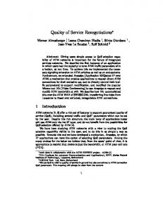
That limit, smax, is computed to be 24. Thus, it is theoretically possible to support 24 such MPEG-1 video streams using the proposed scheduling strategy. What of the bu�er requirement? Figure 2.2 plots Bmin , the minimum bu�er needed to service s MPEG-1 video streams.
x 10
4
Buffer Requirement at the CMS
9 8
Minimum Buffer Required
7 6 5 4 3 2 1 0 0
5
10 15 Number of MPEG-1 video streams
Figure 2.2: B(in KB) vs. s
20
25
19 The interesting observation from Figure 2.2 is the non-linearity of the Bmin curve. In our example, this means that to service a relatively large set of streams, i.e. upto 23 MPEG-1 video streams, about 88MB of bu�er is su�cient. However, if a 24th stream is added then a minimum of 972MB is neccessary! This steep rise in Ps v r i i bu�er requirement occurs as i=1 b ! 1. In other words, as the playback load approaches the total available I/O throughput, the bu�er requirement increases sharply, i.e. in a non-linear fashion
2.4 Admission Control Corollary 1 can also be used to derive the bu�er condition for admission control, i.e. the condition under which a new stream requested by a client can be serviced by the disk. O(sP ) Psi=1 ri � Bavail 1 ? si=1 vibri 2 Integrating the I/O bandwidth constraints and bu�er constraints yields the condition for admitting a stream. If Bavail bytes is the maximum available bu�er then stream (s +1), with play-out rate rs+1 and per block access time vs+1, can be admitted only if sX +1 vi ri i=1 b{z |
(
< 1) }
sX +1
^ ( 2bni � Bavail) i=1 |
{z
(2.8)
}
I/O bandwidth limitation bu�er limitation The request for admission is rejected if by admitting the new stream Condition 2.8 is violated.
2.5 The Bu�er-Slack Trade-o� In BUFMIN CPCC the objective was to minimize the bu�er requirements of BSCAN. When extra bu�er is available to the scheduler it may be traded for increased slack time, i.e. time within each cycle, which may be used to service other (non-real) time accesses to the disk In this section we brie y evaluate the trade-o� between bu�er and slack time. 0 are two feasible solutions to BUFMIN CPCC such that Ps n0 > If n and n i=1 i Ps 0 is the larger schedule, then we can derive the cost of accumulating n , i.e. n i i=1
20 additional slack time. Let S (n) be the slack time at the scheduler when servicing n. If Tsvc is the cycle duration, � � ? O(s) + vT Tsvcb r S (n) = T| {zsvc} cycle duration | service {zduration } We can derive the expression for the increased slack time in each cycle as follows.
S (n0 ) ? S (n) = Or,
s
0 ?T ) 1 ? vibri (Tsvc svc i=1 X
!
s vi(n0i ? ni ) 1 ? vibri i=1 i=1 In other words, if nopt is an optimal solution and n is a larger but feasible solution where
S (n0 ) ? S (n) =
s
X
!
X
n = nopt + p Now, the additional slack time, �S (p), obtained in exchange is s
s v i ri �S (p) = 1 ? v i pi i=1 b i=1 X
!
X
(2.9)
Equation�2.9 isPinteresting because the additional slack time �S (p) isPweighted by � s v r the term 1 ? i=1 ib i . This implies that as the disk gets loaded, or si=1 vibri ! 1, the returns, in terms of slack, from investing additional bu�er (larger p) rapidly diminishes. Conversely, if P a certain amount of slack time must be maintained at the disk then the value of si=1 vibri must be restricted to a smaller range than that given by Condition 2.8.
2.6 Open Issues The mathematical model for the scheduler can be enhanced to include a comprehensive disk model, a general service order within a cycle, and exploit features in newer disks like zoned bit recoding or ZBR [Tewari et al., 1996]. While incorporating these aspects will make the scheduling model more accurate the analysis becomes
21 complex which, in some cases, may not be worthwhile. In this section we state the rami cations of incorporating these issues and report them as open problems.
2.6.1 Seek Model
Recent investigation by [Ruemmler and Wilkes, 1993] shows that disk seek times can be piece{wise approximated analytically. Instead of the non{linear cost model assumed in Lemma 1, they conclude the following seek model to be closer to actual disks: (
p
�1 tr; if tr � C; � (tr) = ��0 + (2.10) otherwise. 2 + �3 tr; where �0; �1 ; �2; �3 and C depend on the speci cs of a disk. Deriving a result similar to Lemma 1 using this updated disk model is an open problem.
2.6.2 A Generic Service Model In BSCAN, blocks of a single stream were assumed to be fetched in batches while
di�erent streams were assumed to be serviced in SCAN order. In a more general service model, all blocks of data within a cycle may be assumed to be fetched in SCAN (or CSCAN) order. This leads to a more involved cost model. We formulate this problem here. From Lemma 1 the service time overhead for servicing s requests using SCAN is bounded as s
O(s) � (s ? 1)(�0 + �1 s ?T 1 ) + stmax rotation Using a general service model there will be eT n blocks to be fetched in SCAN
order in each cycle. Thus,
O(eT n) � (eT n ? 1)(�
s
0 + �1
To prevent starvation we must ensure that
T
eT n ? 1 ) + e
T ntmax rotation
bn � (O(eT n) + vT n)r Simplifying this expression leads to, q
T T bn � r((�0 + tmax rotation )e + v) n + �1 T (e n ? 1) ? �0
22 Note that this is a quadric expression which is di�cult to solve. The solution to this general form of BSCAN is an open problem.
2.6.3 New Disk Features Two new emerging features in disks are (i) manual thermal recalibration, and (ii) ZBR. Most disks need to perform periodic recalibrations. During recalibrations no disk I/O can proceed and hence should be factored in computing the cycle time. However, recent disks allow manual calibration wherein recalibrations can be demand driven. This allows the addition of su�cient slack at the scheduler to perform periodic calibrations. An alternative is to model and include recalibration times in the cycles. A more signi cant development in storage disks is the introduction of ZBR [Tewari et al., 1996]. Due to geometric considerations the outer tracks of a sector can store more data than the inner ones. However, due to CAV, older disks were unable to exploit this and read data at a constant rate R regardless of the current head position. Recent disks have zone based read rates, i.e. the read rate Rinner for inner tracks can be upto 60% of the read rate Router for outer tracks. This impacts Equation 2.1 since R is no longer constant. Consequently, the problem of deriving a result similar to Lemma 1 using zone read rates remains open.
2.7 Summary We developed the BSCAN scheduling scheme to ensure continuity and meet realtime access requirements of CM data. We derived a schedulability condition that proves that BSCAN is able to utilize upto 100% of the retrieval bandwidth. However, bu�er requirement with BSCAN grows non-linearly with load. An admission control condition was developed to ensure that both bu�er and bandwidth are not exceeded. A trade-o� in bu�er and slack time was demostrated and quanti ed. This trade-o� is key and will be employed in subsequent chapters. Much of the analysis in this chapter can be described as the steady state analysis of the scheduler since it does not considered dynamic changes to the system variables.
Chapter 3
Implementation Constraints for the Scheduler BUFMIN CPCC is a theoretical formulation of the bu�er minimization problem and overlooks some fundamental constraints in scheduling accesses to the disk as well as in clients' data consumption pattern. In this chapter we motivate the need to capture these additional constraints, and develop solutions to ensure a feasible implementation of the scheduler. A fundamental constraint of a disk is that data accesses must be in integral multiples of the physical block size. For example, it is not possible to fetch 4.37 blocks since it involves fetching a fraction of the 5th block. Thus, while n� is the solution to BUFMIN CPCC , in most cases it will be infeasible to service such a schedule. In order to ensure that the computed schedule is feasible, additional constraints are added to BUFMIN CPCC to derive problem BUFMIN DPCC . Its formulation and solution are discussed in Section 3.1. The second fundamental assumption made in BUFMIN CPCC is that a client's consumption proceeds at a constant and continuous rate. Such an assumption is justi ed for streams that have small sample sizes. Audio streams typically have 2 byte samples can be modelled by a constant and continuous data rate. In case of video streams this assumption is not justi able. A video stream is typically a sequence of frames (large sample size) and the decoders/frame{bu�ers require the entire frame periodically. Thus, the consumption rate is not continuous, but discrete and proceeds in steps, with a step at each time an entire frame is consumed. At the time of decompression/rendition data corresponding to the entire frame must be in the main memory, else the decompression/rendition will be delayed. Thus, it is neccessary to ensure that the entire frame is available in bu�er at the time of consumption. These additional constraints to BUFMIN DPCC result in problem BUFMIN DPDC that is formulated and solved in Section 3.2. Finally, in Section 3.3, the scheduling strategy is extended to handle variable data rate streams. Data rate variability is caused because of data compression and a technique to adapt BSCAN to handle this data rate variability while ensuring smooth playback is discussed. In Section 3.4 the analytical model is validated via simulation studies.
23
24
3.1 Schedules with Integral Entries In this section we derive schedules with integral entries, i.e. schedules that require fetching integral multiples of blocks from the disk in each cycle. These additional constraints transform the bu�er minimization problem to BUFMIN DPCC (formally stated below), the integer linear programming (ILP) version of BUFMIN CPCC .
Problem 2 (BUFMIN DPCC ) min B = 2b
s
X
i=1
ni
such that
Mn � O(s)r ni � 0 and is an integer for all 1 � i � s.
Various techniques to solve ILPs have been proposed in [Luenberger, 1984], [Greenberg, 1971]. Again, the special structure of BUFMIN DPCC allows us to derive its solution from that of P1. Henceforth in this dissertation we denote the solution of BUFMIN DPCC as n+ . A simple technique to derive the solution of BUFMIN DPCC from the solution to BUFMIN CPCC is to apply an integer function like oor(b c) and ceiling(d e) on n� . For example, given the optimal schedule n� (from BUFMIN CPCC ), dn� e is a possible derived schedule obtained by applying the ceiling function to each entry in n� . In fact, dn� e is the solution of BUFMIN DPCC under certain restrictions. This is proved in the following lemma. In the lemma, streams are similar if they have identical playback rates, and inter block access times, but di�er in content.
Lemma 3 When streams are similar, i.e. r1 = ri = r and v1 = vi = v, n+ = dn� e. Proof: The claim is proved in two steps: (i) dn� e is shown to be a feasible solution to BUFMIN DPCC , and (ii) dn� e is the optimal solution to BUFMIN DPCC . (i) Let
dn� e = n� + fn� g
Or, fn�i g is the fractional part added to n�i by applying the ceiling function. Since all streams are similar, fn�i g = fn�j g = fn� g. From Theorem 1 we have b > svr. Or, � r < svbffnn�gg
25 Or, �g b f n 8i; ri < vT fn� g
This implies that Mfn� g > 0. Since Mn� = O(s)r we have,
M(n� + fn�g) > O(s)r
which means that dn� e is a feasible solution to BUFMIN DPCC . (ii) To prove the optimality of dn� e, recall that any solution for BUFMIN DPCC has to be greater (element-wise) than n� (Theorem 2). Since dn� e is the smallest vector with integer entries that is greater than n� , dn� e is optimal. Although the application of the result in Lemma 3 is limited (it works only if all the streams have similar playback rate and placement) it is quite useful in cases where the disk is con gured to store similar streams. Such a disk stores stream instances of a single type, e.g. MPEG-1 compressed video streams. Such con gurations will be popular for Video-On-Demand applications where di�erent video stream instances will be stored in a uniform compression standard which would include playback at similar rates [Tobagi et al., 1993], [Chang et al., 1994], [Bolosky et al., 1996]. When con gured to store dissimilar streams, the disk must store streams compressed using di�erent standards and playback rates. In such a case the schedule due to Lemma 3 will neither guarantee feasibility nor optimality for BUFMIN DPCC . Previous attempts at deriving schedules whose entries are integral multiples can be found in [Rangan and Vin, 1993a]. It proposes the use of ceilings and oors. In [Kenchammana-Hosekote and Srivastava, 1994b] a detailed analysis of using dn� e and bn� c is carried out. The signi cant result from that was that simple use of ceiling and oor functions to derive schedules with integer entries can result in jitter or rate variation during retrieval { an undesirable e�ect during playback. � In cases where there exists a stream i such that ri > vbTffnni �gg , dn� e will be infeasible. Suppose the example disk of the previous chapter (Section 2.3.2) is required to schedule 4 motion-JPEG video streams, each of which requires a playback rate of 900KBps (30KB per frame at 30 frames per second), and one MPEG-1 video stream. The schedule computed by such a derivation from Theorem 2 requires dn�JPEGe = 553 blocks for each JPEG stream and dn�MPEGe = 111 blocks for the MPEG-1 stream, to be retrieved in each cycle. However, such a schedule is infeasible since in executing the derived schedule, the motion-JPEG streams will have jitter during playback which will grow over time as the stream gets rendered. Thus, a general and systematic method of deriving the solution of BUFMIN DPCC from that of BUFMIN CPCC is neccessary. In fact, for the general case, any feasible solution to BUFMIN DPCC
26 will be of the form dn� e + p, where p is a vector with integer entries (See proof of Theorem 1). The general solution of BUFMIN DPCC is stated in the following theorem:
Theorem 3 The solution of BUFMIN DPCC is n+ where n+ = dn�e + p�
and the vector p� is computed by the algorithm1 PSTAR.
Algorithm 3.1 PSTAR .
Algorithm to derive p� .
1 p 0; 2 �p 0; 3 do 4 p p + �p;
. Compute the cycle duration for Tsvc (s) + vT ( n� + p); . � is the data de cit due to d Tsvc r ( n� + p) ; �p
5
p
6 7
O
d
d e
?d e
b
e
dn� e + p.
n�e + p.
until ( �p = 0); 8 p� p;
Proof: The claim is proved in two steps: (i) dn� e + p� is shown to be a feasible solution, and (ii) dn� e + p� is shown to be optimal. (i) To show that dn� e + p� is feasible note that at the end of PSTAR, �p = 0. Or,
If e = (1; : : : ; 1)T then, Or, Or,
� � d Tsvc b r ? (dn e + p )e = 0 � � 0 � Tsvc b r ? (dn e + p ) > ?e
0 � O(s)r + rvT (dn� e + p�) ? b(dn� e + p�) > ?be be > M(dn� e + p� ) ? O(s)r � 0
1 The author would like to apologize for the unconventional statement of this theorem. The use
of an algorithm in the statement was necessary because of the lack of a closed form solution to BUFMIN DPCC .
27 Thus, M(dn�e+p� ) � O(s)r, or dn� e+p� is a feasible solution of BUFMIN DPCC . (ii) dn� e + p� is the optimal solution of BUFMIN DPCC : (By contradiction). Assume that there exists p0 where, p� = p0 + �p and there exists an i such that �pi > 0 and all pi's are integers. Consider the expression E
E = M(dn� e + p0 ) ? O(s)r Substituting p0 = p� ? �p, From (i) Hence,
E = M(dn�e + p� ? �p) ? O(s)r be > M(dn� e + p� ) ? O(s)r � 0
be ? M�p > E � ?M�p If dn� e + p0 is to be feasible, E � 0 or,
?M�p � 0
Since M is invertible and M?1 has non-negative entries,
M�p � 0 ) �p � 0
Or, 8i; �pi � 0. This is a contradition.
PSTAR is a search algorithm in the subspace of Rs. However, unlike other search algorithms, e.g. [Anderson et al., 1992], PSTAR starts searching from dn� e since the solution of BUFMIN DPCC is guaranteed to be no smaller than n� . The algorithm initially starts with p set to 0. In each iteration (lines 4{7) the algorithm tests the feasibility of the schedule dn� e + p. If the current schedule is infeasible it computes the potential data de cit �p (line 6), had the scheduler executed that schedule. The algorithm then increases the current schedule dn� e + p by �p and searches from there on until it reaches a feasible schedule. Notice that as the schedule length is increased in each iteration, the e�ective throughput from the storage system increases. PSTAR applied to our example disk yields the optimal schedule, n+JPEG = 554 blocks and n+MPEG = 111 blocks.
28
3.2 Schedules for Frame Oriented Streams In this section we re ne BUFMIN DPCC to handle scheduling of frame oriented streams, i.e. streams where playback involves rendering chunks of data blocks at discrete points in time. Until now the clients' rates of consumption were expressed in bytes per second implying continuous consumption, i.e. if a client consumed data at rate r, then in a time interval �t it will consume r�t bytes. In reality, clients consume samples at xed time intervals. When these samples are small, as in an audio stream, the consumption rate can be approximated by a continuous rate without causing any perceivable undesirable e�ect during playback. However, the same cannot be said when streams have signi cantly large sample sizes, as in video streams. In such streams playback involves periodic rendering of frames, each of which may span multiple disk blocks. At the time of rendition all blocks of the frame must be available to the decoder/frame-bu�er. If the entire frame is unavailable, then the decoder/frame-bu�er stalls introducing jitter in the playback. In essence, to schedule frame oriented streams, it is not just su�cient to execute schedules with integer entries. Such schedules must ensure that su�cient data corresponding to all frames to be rendered is available in the clients' bu�ers to ensure timeliness during playback. Let ui be the size (in disk blocks) of each frame in stream i. Consequently, the client's playback rate for stream i is assumed to be �i (in frames per second). Thus, over the entire playback period
ri = b�i ui (3.1) In the time to service each cycle of duration Tsvc seconds, the client can consume atmost dTsvc�i e frames. For example, if a client was playing back a motion-JPEG video stream at 30 frames per second and the service cycle was 50 ms then no more that d0:05 � 30e = 2 frames will be consumed in any cycle. Thus, for a frame oriented stream i in each cycle,
8i;
ni � dTsvc �ieui blocks in bu�er frames(in blocks) consumed In order to accomodate frame oriented streams, the constraints in BUFMIN DPCC need to be modi ed. This modi cation results in problem BUFMIN DPDC formally stated below. |{z}
|
Problem 3 (BUFMIN DPDC ) min B = 2
s
X
i=1
bni
{z
}
29 such that
8i; ni � d(O(s) + vT n)�ieui
and all ni's � 0 and integral.
Unlike BUFMIN CPCC and BUFMIN DPCC , the constraints in BUFMIN DPDC cannot be compactly written in vector notation because of the ceiling function. Furthermore, BUFMIN DPDC is not an ILP since the constraints are no longer linear. However, the special structure of BUFMIN DPDC allows us to compute the solution using the solution of BUFMIN DPCC . If we denote the solution of BUFMIN DPDC as nu+ then the following result holds:
Lemma 4 nu+ � n+ Proof: By contradiction. Suppose n+ = nu + + � n such that �ni > 0, for some i. Since n+ is the solution for BUFMIN DPCC , Mn+ � O(s)r
Or, Substituting ri = b�i ui,
M(nu+ + �n) � O(s)r
8i; nu +i ? (O(s) + vT nu+)�i ui + (�ni ? �iuivT �n) � 0 Also, since nu + is the solution to BUFMIN DPDC , 8i; nu +i ? d(O(s) + vT nu+)�i eui � 0
For Expressions 3.2 and 3.3 to be simutaneously true, we require that
8i; 0 � �ni ? �iuivT �n > ((O(s) + vT nu +)�i ? d(O(s) + vT nu +)�ie)ui Or,
0 � M�n > ?u
Or 8i; �ni � 0 which is a contradiction. Hence the claim.
(3.2) (3.3)
30 This validity of this result can be argued by intuition. The duration of a cycle for frame oriented streams is bound to be longer than that in BUFMIN DPCC since entire frames need to be fetched. Longer cycles require larger set of blocks to be bu�ered and thus the observation. Given this result, solution to BUFMIN DPDC can be assumed to be of the form nu + = n+ + p, where p is a vector with integer entries. Theorem 4 provides the general solution of BUFMIN DPDC .
Theorem 4 The solution of BUFMIN DPDC is nu + where nu + = n+ + pu �
and the vector pu � is computed by the algorithm2 PU STAR.
Algorithm 3.2 PUSTAR .
Algorithm to derive pu � .
1 p = 0; 2 �p 0; 3 do 4 for i 1 to s 56 pi pi + d�pi ui e; 7 end 8 9 11 10 12 13 14
n
p.
. Compute the cycle duration in servicing + + Tsvc (s) + vT (n+ + p); . � is the data de cit due to servicing + + .
for
p
O
i 1 to s �pi dTsvc �i e ? (ni u+i pi ) ;
n
p
+
end
until ( d�pe � 0); p� p;
Proof: The proof of this claim closely follows that of the proof for Theorem 3. As before, the proof is developed in two steps: (i) nu + is shown to be a feasible solution of BUFMIN DPDC , and (ii) nu + is shown to be optimal. (i) nu+ is feasible: When PUSTAR terminates, d�pe = 0. Or, Or, 2 See note for Theorem 3.
8i; n+i + pu�i ? dTsvc�i eui � 0
31
Or,
8i; n+i + pu�i ? d(O(s) + vT (n+ + pu �)�ieui � 0 8i; nu +i � d(O(s) + vT nu+)�i eui
Hence, nu + is feasible. (ii) nu+ is optimal: From (i) nu + satis es Or,
8i; n+i + pu�i ? d(O(s) + vT (n+ + pu �)�ieui � 0
Since ri = b�i ui,
8i; n+i + pu�i ? (O(s) + vT (n+ + pu �)�iui � 0 Mnu+ ? O(s)r � 0
(3.4) nu + is proved to be optimal by contradiction. Suppose pu� can be written as
pu � = pu 0 + �p
such that �pi > 0 for some i. Then consider the expression Substituting for pu 0, Using Equation 3.4
E = M(n+ + pu 0) ? O(s)r E = M(nu+ + pu � ? �p) ? O(s)r E � ?M�p
Since n+ + pu 0 is feasible, E � 0, for which we require that
?M�p � 0 ) �p � 0
Or,8i; �pi � 0 which contradicts our assumption. Hence, nu+ is optimal.
PUSTAR searches the feasible subspace of BUFMIN DPDC in the same way that PSTAR searches the space of integer points of BUFMIN DPCC . In each iteration, PUSTAR checks the feasibility of n+ + p. If the current schedule is infeasible, it
32 computes the data de cit, if the current schedule were executed, as �p. In the next iteration it increases the schedule for stream i by �piui and repeats until a feasible point is reached. Notice that as long as 8i; ui � b, i.e. the size of each frame of all s streams is less than or equal to the block size, the solutions of BUFMIN DPCC and BUFMIN DPDC will be identical. Admission control when scheduling frame oriented streams can be derived from condition 2.8 by making the substitution given in Equation 3.1. Thus, as long as sX +1
(
i=1 |
vi�i ui < 1) {z
}
sX +1
^ ( 2bnu+i � Bavail) i=1 |
{z
(3.5)
}
I/O bandwidth limitation bu�er limitation stream (s + 1), with playback rate �s+1 and frame size us+1, may be admitted.
3.3 Schedules for Compressed Streams In this section we compute schedules for variable data, constant frame rate streams. Data rate variability in the playback of such streams occurs mainly because of compression of frames. The compressed frames vary in size depending on the content and compression techniques. For example, Figure 3.1 shows the variation of the data rate over time for a motion-JPEG3 video stream [Wallace, 1991]. x 10
4
Frame Size Distribution for PILOT.JPG
2
1.8
1.6
Size (in bytes)
1.4
1.2
1
0.8
0.6
0.4 0
100
200 300 400 Frame Number (or time in 83ms intervals)
500
600
Figure 3.1: Frame Sizes in a motion JPEG stream. 3 The data was collected for a 640x480 motion-JPEG video stream from a Parallax Video board at
a capture rate of 12 frames per second and a QFactor= 90.
33 When playback of streams have data rate variability, in order to maintain jitterfree playback, we must take a conservative approach in the allocation of resources (here the I/O bandwidth), i.e. based on the largest frame sizes. Such playback guarantees are required in many mission critical applications like command and process control in defense [USAF, 1994] and industry [Guha et al., 1993], and in domains like medicine [ACM, 1995] and sound production [Pohlmann, 1995]. Our approach to providing jitter-free playback rate of VBR streams is to provide I/O bandwidth corresponding to playback at the highest data rate. The unused bandwidth is dynamically allocated to service clients who do not require playback guarantees and/or to schedule non-real time accesses to the storage system. However, since bandwidth is allocated based on peak playback rate, we must ensure that executions of successive schedules do not lead to bu�er overruns. In the rest of this section we shall discuss our approach to scheduling such streams. In the rst step we derive the schedule for the worst case, i.e. when all s streams require their maximum data rate. This is done by selecting ui to be the maximum + frame size umax i . The schedule, nu , computed with such an assumption is used as the basic schedule. Due to variation in frame size, blocks fetched in cycle k will not be completely consumed in cycle k + 1. If Bik is the number of blocks of stream i remaining at the end of cycle k, then this remainder data may be used to reduce the service vector for the cycle k + 1. In other words,
nk+1 = nu+ ? bBk c (3.6) Since B0 = 0, the schedule starts with n1 = nu +. Subsequently, Equation 3.6
is used to compute the e�ective schedule. Since the e�ective schedule in any cycle will be less than or equal to nu+ , there is some slack bandwidth that goes unutilized. This bandwidth may be used to service clients for non-real time data accesses. A simple implementation of this approach can be done using a circular bu�er for the double bu�er organization. Bu�er space of 2nu+i blocks is arranged as a circular bu�er for stream i. Two pointers are maintained, one for consumption (the consumer pointer), and another for production (the producer pointer). For retrieval, the client updates the consumer pointer while the scheduler updates the producer pointer. In this way, frame fragmentation4 and subsequent re-arrangement is avoided. The technique described here can be extended to handle inter-frame coded streams like MPEG. Figure 3.2 shows frame sizes of a typical MPEG-1 video stream. The additional problem in scheduling data for such streams is that to decompress a frame, 4 A frame is fragmented if it is not stored in contiguous (virtual) memory. Commercially available
video cards like Parallax and SunVideo require unfragmented frames for display. Fragmented frames need to be re-arranged into contiguous memory and require movement of data of at most half of a frame.
34 Frame Size Distribution for US.MPG 14000
12000 I frames
Size (in bytes)
10000
8000 P frames 6000
4000 B frames 2000
0 0
100
200
300 400 500 600 Frame Number (or time in 83ms intervals)
700
800
Figure 3.2: Frame Sizes in a MPEG Stream. especially the P and B frames, the decoder requires additional frames. In For example, these dependencies for an interleaved sequence of I1B2B3P4B5B6 sequence are: Frame B3 requires frames I1 and P4 to be retrieved before it can be decoded. Thus, in addition to requiring the entire frame to be bu�ered for decompression, each frame in a MPEG stream requires all frames that it depends on to be bu�ered before it can be decoded. In some interleaving schemes of MPEG the stream comprises solely of I frames. In such cases the scheduling is no di�erent from that used for motion-JPEG video streams. When the MPEG stream has B and P frames, a set of frames that can be independently decoded, a group in MPEG [ISO/MPEG Committee, 1990], is assumed as the frame size. Thus, in our example the sequence IBBPBB comprises a group and this entire set of frames are assumed to be a single unit for generating schedules. The frame size ui is set to the size of the group in stream i and the playback rate �i set to 5 groups a second for a 30 frames per second playback.
3.4 Experimental Evaluation In this section we validate our analysis of BSCAN via simulation studies. In the following sections we describe the experiment set up, data collection techniques, load generation, capacity analysis, and experiments validating the analytical model.
3.4.1 Experiment Set Up The experiments presented here were conducted using MAGELLAN, a simulator described in detail in Appendix D and [Kenchammana-Hosekote, 1995]. For results presented in this chapter, MAGELLAN simulated a disk with parameters described in
35 Table 3.1. This con guration corresponds to a Sun Sparcstation 20 with a Seagate Barracuda 2GB disk with Parallax video card playing back motion-JPEG compressed video streams. Parameter Block size b Total Tracks T RPM tmax rotation Capacity of 1 track Transfer rate R Per block Access v Fixed Component �0 Variable Component �1 JPEG Frame Resolution JPEG Frame size u JPEG Frame rate �
Value 2048 bytes 2800 tracks 5400 rpm 11.11 msec 48MB 4.42 MBps 0.49 msec 0.005 sec 0.001 sec/track 640x480 � 9.004 blocks 12 fps
Table 3.1: Simulation Parameters for MAGELLAN. To simulate frame-oriented streams we collected motion-JPEG video streams from the Parallax card on the Sparc 20. Frame size statistics, collected from video clips recorded with the Parallax card, are also summarized in Table 3.1. In the experiments the track location of a stream was assumed to be uniformly distributed over [0; T ? 1]. On request by a client, a video stream is started at the server by suitably altering the I/O schedule. In each cycle the I/O scheduler at the server periodically submits the BSCAN schedule to the disk simulator. The simulator services the schedule in SCAN order. Data fetched from the disk is moved into a bu�er manager that maintains a circular bu�er for each retrieved stream.
3.4.2 Data Collection While collecting data for each run a warm-up time was allocated wherein no data was collected. This was to avoid transient e�ects due to start up. Note that in executing the rst cycle at the scheduler, data is fetched from the storage system and no data is consumed in that cycle. From the 2nd cycle onwards the clients' consumption proceeds. This initial transient phenomenon is avoided by selecting a warm-up time of 5 cycles. We found that the e�ect due to transients was minimal
36 (to absent) after this duration. Data was collected over a period of 500 cycles. We chose to de ne the simulation duration in cycles rather than time units because all statistics were sampled at the end of each cycle. By keeping the number of samples collected per statistic per run constant a fair comparision was possible. The runtime was selected to be 500 cycles after it was observed that there was no signi cant variation in measured statistic if run longer. For every run each statistic collector typically maintained the sample mean, sample variance, a 95% two sided con dence interval, sample order statistics, i.e. maximum and minimum, of the variable it was entrusted to monitor.
3.4.3 Metrics Measured and Summarization Rules We supply a summary of de nitions for the metrics that were measured and reported in the experiments. These metrics may be classi ed broadly into two classes for purposes of data collection | (i) Scheduler metric is one which is measured for the scheduler, and (ii) Stream metric which is measured for a stream. Scheduler metrics include disk utilization and slack, and the stream metric reported here is bu�er utilization. 1. Disk Utilization (scheduler metric): The fraction of time spend doing useful work. The time spend by the disk was classi ed in the simulations into the seek time, rotational latency, and transfer time, and slack/idle time created because of data over fetched from a previous cycles (Equation 3.6). 2. Slack (scheduler metric): The fraction of the time in each cycle that was allocated, but wasted. Slack time is unusable for scheduling CM stream accesses but can be used to service non real-time accesses to the disk. 3. Capacity (scheduler metric): The maximum number of reference streams that could be supported by the server. For experiments reported here this reference stream was pilot.jpg (Figure 3.1). 4. Bu�er Utilization (stream metric): The amount of main memory used to service the stream is measured at the end of every cycle. In every run we get one sample for each of the scheduler metrics. For every stream metric, each run yields the sample count, mean, variance, and 95% two sided con dence interval. In order to report statistics for both scheduler and stream metrics for each experiment from 8 runs, we used a summarization rule that is brie y described here.
37 If the statistic was a scheduler metric (utilization and slack), then an arithmetic mean and a 95% two sided con dence interval for the statistic was computed from all runs. Since the cycle duration for all runs is constant, the use of arithmetic mean is justi ed [Smith, 1988]. If the statistic was a stream metric, then the statistic with the most number of samples was chosen. We chose this scheme because there is greater con dence in a statistic computed from a larger sample. In case two or more runs had the same number of samples, the one with the larger (The choice of picking the larger or smaller value depended on the type of metric. If the metric was a higher the better (HTB) metric [Jain, 1991], then the smaller value was chosen and if lower the better (LTB), then the larger value. Bu�er utilization is a LTB metric and hence the choice of the larger value.) mean was selected. If there were more than one statistic with equal mean, then the statistic with the smaller con dence interval was chosen.
3.4.4 Load Generation Load at the disk was simulated by introducing identical instances of pilot.jpg (Figure 3.1). We chose to use identical streams such that variation in the measured metrics were controlled. The video clip pilot.jpg was a 50s, 640�480 pixel, 16-bit motion-JPEG clip recorded at 12 frames per second from a Parallax Video Card on a Sparc 20. The clip had sample mean frame size � = 9:47 KB, sample variance �2 = 1:224, sample maximum umax = 18:008 KB, and sample minimum umin = 4:32 KB. In order to simulate playback of a constant frame size stream the worst case frame size umax = 18:008 KB of pilot.jpg was chosen. Thus, for Experiments 1 and 2 each stream was a constant frame size (18.000KB) played back at a constant frame rate of 12 frames per second. In order to simulate variable data rate streams, a truncated normal distribution was t to the trace data.
3.4.5 Capacity Analysis For the simulated con guration we were able to compute from Condition 3.5 that a maximum of 19 instances of pilot.jpg could be simultaneously supported with 68.875 MB of main memory.
38
3.4.6 Experiments Experiment 1: Bu�er Utilization with BSCAN.
Bu�er Utilization (in 2K Blocks)
The aim here was to compare the bu�er utilization from simulations with theoretically derived values from the mathematical model. Figure 3.3 plots the experimental bu�er utilization (with 95% two sided con dence intervals) against the load. For comparison the theoretical values for bu�er utilization are also plotted in the gure. Observe that the observed bu�er utilization curve in Figure 3.3 follows the theoretically derived values closely. 160 140 120 100 80 60 40 20 0
Storage System Utilization vs. Load Observed� n n+i+i nu
2
4
6
8 10 12 14 16 Load (number of streams)
18
20
Figure 3.3: Bu�er utilization for a stream vs. o�ered load.
Experiment 2: Disk Utilization with BSCAN
The intent of this experiment was to study the disk utilization with BSCAN. Since utilization is de ned as the ratio of time spent doing useful work and the total elapsed time at the scheduler, this metric gives a measure of how well the I/O scheduler keeps the disk busy. Note that higher the utilization, lower is the slack, which is a measure of the excess but unusable I/O bandwidth and bu�er allocated by the scheduler. To satisfy the additional constraints discussed in this chapter some nite slack is introduced. In Figure 3.4 the disk utilization (with 95% two sided con dence intervals) is plotted against the load.
39 From Figure 3.4 we notice that under light load conditions (2{5 streams) disk utilization with BSCAN is below 70%. However, in regions of medium to heavy load BSCAN maintains disk utilization well above 80%, and asymptotically converges to 100% utilization at peak capacity. The reason for this behaviour is the cost model of access time to the disk. Under light load conditions, the seek time makes up for a large fraction of the total cycle duration. In addition, the extra data added to the schedule to satisfy the integral constraints introduce signi cant slack. Thus, under light load conditions, the disk utilization tends to be low. However, with increase in load, the fraction of time spent in seeks decreases, as does the additional data fetched to satisfy the integer constraints. These two factors contribute to improved utilization with increasing load. To further illustrate this point, Figure 3.5 presents the distribution of time spent in a cycle at di�erent loads. Storage System Utilization vs. Load 1
0.8
Utilization
0.6
0.4
0.2
0 2
4
6
8
10 12 14 Load (number of streams)
16
18
20
Figure 3.4: Disk utilization vs. o�ered load.
Experiment 3: Scheduling Variable Data Rate Streams with BSCAN The aim of this experiment was to study the performance of BSCAN when schedul-
ing variable data rate streams (Section 3.3). Figure 3.6 plots the disk utilization against the o�ered load. From the gure we note that under light load conditions BSCAN progressively improves utilization until this growth peaks, and subsequently deteriorates in regions of heavy load. This trend can be explained by the fact that in BSCAN the cycle duration increases non-linearly with load. With longer cycles the number of frames fetched in each cycle increases. Since the schedule is com-
40 Distribution of Time in a Cycle 1.2
Slack
Transfer
Overhead
1
0.8
0.6
0.4
0.2
0 0
5
10
15
20
Figure 3.5: Distribution of time in a cycle for frame oriented streams. puted based on peak frame sizes, the excess allocation is larger with larger number of frames. This is true because the average frame size tends to the mean and deviate. Consequently, the di�erence between the maximum sample frame size and its mean increases with the size of the sample. Thus, in allocating peak bandwidth for variable data rate streams the utilization decreases with increase in load. Figure 3.7 presents the distribution of time spent in a cycle at di�erent loads when scheduling variable data rate streams. It is clear that slack increases with load, leading to low utilization.
Experiment 4: Bu�er Slack Trade-o� The aim of this experiment was to study the bu�er and slack trade-o� presented in the previous chapter. It was shown that while it is possible to exchange extra bu�er allocation for increased slack time, the bene ts from such an exchange diminish as the load increase. For runs of this experiment the cycle duration was increased (and consequently bu�er utilization) using the following equation
nused = n+u + kdue; k = 0; 1; 2; 4; 8: Figure 3.8 plots the slack against k, the additional number of units fetched in each cycle under di�erent load conditions, i.e. light (5 Streams), moderate (10 Streams) and heavy (15 Streams). Two trends are evident from the gure. The rst is that the slack gained by additional bu�er allocation diminishes with increase in load. This is a consequence of the fact that under heavy load conditions the utilization is high (Experiment 2). The second trend involves the rate of increase of slack (seen in the gure as the slope of each of the load lines). Lower rates are observed under heavier
41
Load vs. Storage System Utilization 1
0.8
utilization
0.6
0.4
Fixed Frame Size Variable Frame Size
0.2
0 0
5
10 Number of motion-JPEG Video Streams
15
20
Figure 3.6: Disk utilization vs. o�ered load for VDR streams.
Distribution of Time in a Cycle 1.2
Slack
Transfer
Overhead
1
0.8
0.6
0.4
0.2
0 0
5
10
15
20
Figure 3.7: Distribution of time in a cycle for VDR streams.
42 load conditions. This supports the observation made in the previous chapter that the bene ts of increasing bu�er allocation in exchange for slack diminishes with heavier loads. Slack vs. Buffer 0.5 Light Load Moderate Load Heavy Load
0.45 0.4 0.35
Slack
0.3 0.25 0.2 0.15 0.1 0.05 0 0
1
2 3 4 5 6 k (number of additional frames fetched in each cycle)
7
8
Figure 3.8: Slack vs. k.
3.5 Related Work The problem of scheduling accesses to I/O systems has been studied extensively as early as [Frank, 1969], [Teorey and Pinkerton, 1972], and [Fuller, 1975]. More recently, [Abbott and Garcia-Molina, 1990] and [Chen et al., 1991] have addressed the problem in the context of real-time systems. With the growing interest in continuous media server design, recent work by [Gemmell, 1993], [Reddy and Wyllie, 1993], [Chen et al., 1993], [Anderson et al., 1992], [Rangan and Vin, 1993a], [Gemmell and Christodoulakis, 1992], [Lougher and Shepherd, 1992], [Ramakrishnan et al., 1993], [Chang et al., 1994], [Daigle and Strosnider, 1994] [Chen and Little, 1993] have been signi cant. While [Gemmell and Christodoulakis, 1992] presents a general theory of retrieval for continuous media there have been two distinct approaches to the retrieval problem. First, approaches like [Reddy and Wyllie, 1993], [Ramakrishnan et al., 1993], [Tindell and Burns, 1993], and [Daigle and Strosnider, 1994] adapt scheduling algorithms used in real-time systems to continuous media access. [Reddy and Wyllie, 1993] and [Daigle and Strosnider, 1994] give thorough evaluations of these algorithms. An important conclusion has been that larger request sizes coupled with deferred
43 deadlines are the key to performance improvement. This has greatly in uenced our choice of incorporating batching and SCAN features into our scheduling strategy. However, this class of scheduling approaches do not address issues typical of CM data like handling frame-oriented streams. In the second approach, like those in [Gemmell, 1993], [Chen et al., 1993], [Anderson et al., 1992], [Lougher and Shepherd, 1992], [Rangan and Vin, 1993a], and [Chen and Little, 1993] the e�ort has been to derive new scheduling strategies that are aware of the continuous and media requirements. Our work draws heavily on work from the second approach. [Rangan and Vin, 1993a] propose a xed order cyclical scheduling strategy. Their analysis has inspired some of the modelling presented in the previous chapter. Their observation regarding the implementation constraint of integral block fetches inspired the detailed modelling of this constraint. However, they do not address the problem of handling frame-oriented CM data. [Anderson et al., 1992] develop a similar scheduling strategy as that in [Rangan and Vin, 1993a]. However, [Anderson et al., 1992] derive the scheduling strategy by constraining their search of the solution space to integer points. Their minimal feasible WAS algorithm has been made more e�cient as well as has been extended to handle client consumption in discrete chunks called frames. Both [Gemmell, 1993] and [Chen et al., 1993] consider a modi cation to the scheduling strategy rst proposed by [Rangan and Vin, 1993a] and [Anderson et al., 1992]. In their work they consider a mix of a xed order scheduling, with SCAN order servicing of di�erent CM data streams. Their solutions, called group sweep and sorting-set algorithms respectively, involve grouping a set of streams such that groups are serviced in xed order, while SCAN is used within each group. Both works present bu�er minimization algorithms for such a strategy. Their conclusion that performance gains in terms of bu�er space from a mix of xed order and SCAN discipline has in uenced the formulation of BSCAN. Some of the works cited above discuss deterministic services, i.e. playback guarantees are maintained during retrieval. [Chen and Little, 1993] and [Vin et al., 1994] modify round robin scheduling strategies to provide statistical guarantees to clients. In order to better utilize the storage system, they provide a probabilistic analysis of their scheduling models such that most of the times the clients' playback is smooth. Their strategies are useful in domains wherein jitter-free playback guarantees are not neccessary. Finally, work by [Dan et al., 1994] has considered the problem of batching application requests to bene t from the fact that once a stream (or a portion thereof) has been brought into the server's bu�er, techniques such as multi-casting may be used to service a larger number of applications desiring the same stream.
44
3.6 Summary We extended the BSCAN model by incorporating important implementation constraints. Two key constraints are factored into the model { (i) generating schedules with integral entries, and (ii) computing schedules for frame{oriented streams. Both constraints ensure feasible implementation while increasing the complexity of the model. The results of factoring these constraints are demonstrated by simulation experiments. Each of these experiments con rm the predictions from the mathematical model. A modi cation to the BSCAN scheduler was developed to handle variable data rate streams. However, performance evaluation shows that, under heavy load conditions, the utilization of the disk retrieving VBR streams is low.
Chapter 4
Handling VCR Operations In this chapter we study the e�ect of executing VCR operations by clients with the BSCAN scheduler at the disk. We rst de ne a suite of primitive VCR operations that clients can execute to change the ow of CM streams. The e�ect of the execution of such operations with BSCAN is then analyzed. We show that an uncontrolled change in the schedule will a�ect jitter-free playback. In order to avoid breakdown in playback guarantees while executing VCR operations, we develop two general techniques, namely the passive accumulation and active accumulation strategies. Using the response time, i.e. the time to execute a VCR operation, as a comparison metric we show that active accumulation algorithms generally outperform passive accumulation algorithms. We then derive the optimal response time algorithm in a class of active accumulation strategies. Simulation studies are used to validate analytical results presented here. This chapter is organized thus: The classi cation of VCR operations and their e�ect on BSCAN is presented in Section 4.1. In Section 4.2 we discuss the e�ects of executing VCR operations. We then introduce the passive and active accumulation algorithms, as techniques to prevent any transitory e�ect on clients' playback. In Section 4.4 we analyse a class of active accumulation algorithms with the aim of deriving an algorithm with optimal response time. Simulation studies reported in Section 4.5 con rm our ndings.
4.1 VCR Operations Until now it was assumed that r, v, and s remain constant when the schedule was computed, i.e. at some time in the past these parameters had been set and thereafter the scheduler has been executing the schedule periodically. In practice, clients will initiate consumption of data at some (unpredictable) moment, and over the duration of their session they (may) change their consumption rate and/or pattern, and nally after a nite time duration they will end their session. When such changes to the clients' access requests are allowed, the server must make appropriate changes in its operation to satisfy the new requirements, without a�ecting existing clients' jitterfree playback guarantees. In this section we discuss a set of these interactions of the 45
46 clients, that we denote VCR operations, and their e�ect on BSCAN. A client views continuous media as a sequence of data units owing as a stream in real time. For example, in a video stream this data unit will be a frame (uncompressed/ intra-frame compressed JPEG video) or a group of frames (IB � � � P � � � B in inter-frame compressed MPEG video) sequenced in a pre-de ned order at (say) 30 frames per second. In order to change the data ow in such a stream the client can execute one or more VCR operation(s) from a set categorized as follows:
� Rate Variation Operations : Operations in this class change the rate of data units owing in the stream. Since the stream is a timed sequence of data units, this results in a speed-up or slowing of the stream. For example, the VCR operation SlowMotion on a video stream reduces the frame rate of that stream. Thus, if the play out rate was 30 frames per second, then the SlowMotion operation could reduce the rate to 15 frames per second.
� Sequence Variation Operations : An operation that changes the order in which
the data units are owing in the stream belongs to this class. Such operations presume the existence of a (possibly time-stamped) order of data units in the data stream1. For example, the operation FastForward on a video stream may achieve the e�ect by displaying alternate frames and thereby changing the display sequence from the (original) recorded sequence. Notice that the rate at which data units are being consumed can remain unchanged in such an operation. The sequence (and hence the contents) of the frames displayed gives the e�ect of having witnessed a phenomenon in a time interval, which in reality lasted twice the duration.
� Concurrency Set Operations . Operations like Start and Stop which increase
and decrease the number of concurrent streams being scheduled belong to this class. We shall di�erentiate such operations from the rate variation operations shortly.
Henceforth in this paper, we shall represent the set of rate variation operations by Play and ReversePlay, the set of sequence variation operations by ForwardSkip and ReverseSkip, and the set of concurrency set operations by Open and Close. Table 4.1 describes the e�ect of each of these operations on a CM stream S . Other operations like Pause, FastPlay, SlowMotion can be implemented using this set of primitive operations. 1 Such data being discrete samples of a continuous phenomenon are usually ordered by timestamp.
47
4.1.1 E�ect of VCR Operations A VCR operation requested by a client will a�ect the scheduler since it will change the schedule computed with PUSTAR. To understand the e�ect of such an operation we de ne the concept of the state of a scheduler and then relate the execution of VCR operations to changes in scheduler state. Before we motivate the de nition of the state of the scheduler, it is necessary to introduce a measure of the data bu�ered in the main memory at the end of each cycle. Let Bik denote the excess (in addition to the schedule) data blocks bu�ered for stream i in main memory at the end of cycle k, and let Bk be a vector of Bik 's. The state of the scheduler in cycle k is de ned thus: De nition 1 (State of a scheduler) State of a scheduler at the end of cycle k is (nk , Bk ). In other words, the amount of data available for consumption at the end of any cycle k de nes the state of the scheduler. Note,
Bk
|{z}
=
Bk?1
| {z }
+
k r nk?1 ? Tsvc |
{z
}
excess data in new state excess data from previous state accumulation in cycle k (4.1) The state of the scheduler can change with cycles. Such changes can occur when any of the three parameters used in computing nk , i.e. s, r, and v change, since k / nk . Tsvc Rate variation operations modify the consumption rate and hence the vector r. Sequence variation operations change the sequence of data blocks accessed. The required data blocks tend to be spaced farther apart compared to accessing them in the sequence they were stored. Hence sequence variation operations change the vector v, the per-block access cost vector. Concurrency set operations change the number of concurrent streams being serviced by the scheduler. Table 4.1 shows the classi cation of the set of VCR operations and the parameters that consequently change leading to a state change at the scheduler. In the table a set of VCR operations are enumerated along with the parameters that they modify. For example, the Close(S ) operation on a CM stream S reduces the number of concurrent streams at the disk and hence a�ects s. Similarly Play(S ,r) changes the consumption rate of S and thus a�ects the rate vector r. Note that ReversePlay(S ,r) need not a�ect v since the disk scheduler is not constrained to retrieve blocks in the order in which they are to be viewed. Hence, since data fetched in cycle k is not consumed until cycle k + 1, blocks for ReversePlay are fetched in the same sequence as Play with the only di�erence being the order in which data is consumed.
48 VCR Operations Open(S ) Close(S ) Play(S ,r ) ReversePlay(S ,r ) ForwardSkip(S ,skip) ReverseSkip(S ,skip)
Description sp r v Start S with r = 0 p Terminate S whose r = 0 p Play S at rate r p Play S in reverse at rate r p Play S at rate r skipping every (integral) skip units p Reverse Play S at rate r skipping every skip units
Table 4.1: VCR Operations on a CM Stream S . Other operations can be implemented using the primitive operations listed in Table 4.1. For example, Pause(S ) is essentially Play(S ,0). Similarly, FastForward(S ) may be implemented as ForwardSkip(S ,2)2 .
4.1.2 Computing the New State When a VCR operation is invoked by the client, the scheduler needs to compute the new schedule corresponding to that operation, and make a transition (if needed) to the new state. Since from Equation 4.1 a change in the schedule causes change in state, we will discuss the computation of the new state using the schedule. Let n� and nnew be the schedule in the old and new states, respectively. Further, let
nnew = n� + �n Table 4.2 summarizes the expressions for various parameters during a state change due to a VCR operation. Detailed derivations are provided in Appendix C.1. 2 Such an implementation of FastForward implies skipping alternate frames. In cases where streams
are inter-frame compressed MPEG video, a group of frames (IB � � � P � � � B ) is skipped since it is is hard (and possibly meaningless) to skip arbitrarily.
49 Class of Operations Rate Variation Sequence Variation Concurrency Set
Variable Change Lower Bound on �n � � new T r)I + rvT ) �r � = � + �� � (b?vT r)(s� (( b ? v T new b?v r ) � r) vnew = v + �v � (b?vTs�r�)((�b?vTvnewT r) r �s� snew = s + �s b?vT r r
Table 4.2: New State Computation using BSCAN (8i; ri = b�i vi ). It may appear that concurrency set operations can be reduced to equivalent rate variation operations. For example, it appears as if the addition of a new stream should be no di�erent from stepping up its rate from �i = 0, prior to its play out, to some non-zero value. While this equivalence would appear be true for clients, the scheduler needs to di�erentiate between these two operations. The reason for this distinction is that an extra context switch time is required to access data for a new stream. Since disk access time comprises a xed component(seek and rotation) and a variable component(transfer), for the disk, the process of admitting a new stream and that of stepping up the rate of a stream from � = 0 to a greater value are not equivalent.
4.1.3 Admission Control for VCR Operations The scheduler must control the admission of VCR operations based on the availability of the I/O bandwidth and bu�er space. If s
( vinew �new i ui < 1) X
i=1 |
{z
}
s
^ ( 2bnBSCAN � Bavail) i X
i=1 |
{z
(4.2)
}
bu�er limitation I/O bandwidth limitation then the VCR operation is admitted, else the operation is rejected.
4.2 State Transitions Consider a VCR operation op that requires the scheduler in state S to change to state S new . In the previous section we computed the vector nnew corresponding to this new state S new . The next step is the design of an algorithm that will e�ect this state change. Figure 4.1 illustrates a typical state transition at the scheduler.
50 Transient states: fT g State S
State S new
transition profile
Bk nk
k0
t
k0 + c
Figure 4.1: State transition for VCR operation op. In the gure, the horizontal axis measures time. The vertical axis3 measures data available for consumption. The horizontal line at height nk represents data fetched in each cycle prior to cycle k0 + c. Data build-up above this line is Bk , the excess data bu�ered. In changing from state S to S new the scheduler passes through a sequence of transition states, labelled as the set fT g in Figure 4.1. After c cycles the new state S new is reached and the operation op is said to have been completed. Clearly a gamut of algorithms can e�ect the state transition, each possibly enforcing a di�erent criteria for deciding how and when to change states. A seemingly natural way of handling this situation is to immediately step up (or down) the number of blocks fetched in the next cycle. However, in doing so rate guarantee to clients can be violated. Since the fundamental goal of the scheduler is to provide guaranteed data rate to clients at all time, we must select an algorithm that changes states while ensuring that executing VCR operations by one (or more) client(s) does not a�ect the rate guarantee to other clients. If in the new state the cycle duration is larger, then the scheduler must fetch more blocks of data in every cycle. If these additional blocks of data are to be fetched without a�ecting the rate guarantees to other clients, then the scheduler must accumulate su�cient data in bu�ers of other clients before the VCR operation is executed causing the scheduler to resume steady operation in the new state. In 3 By a plot of a vector we imply a set of plots, one for each element of the vector. However, for the
sake of brevity we shall imply, henceforth, any one such plot.
51 Figure 4.1 this is interpreted as follows: Suppose the VCR operation op was requested at the start of cycle k0. In the next c cycles corresponding to the transition states, data is accumulated to reach a level corresponding to state S new , i.e. Bk +c � �n. The shaded region in Figure 4.1 shows the pro le of data accumulation in the transition states. We call this pro le the transition pro le for state change. In e�ect, the VCR operation is executed only after cycle k0 + c. Notice that the time taken to execute the intermediate c cycles is the response time for the VCR operation since it is the time elapsed from the time of its invocation to its actual execution. If in the new state the cycle duration is smaller, then the scheduler needs to reduce its service vector in the subsequent cycles. Figure 4.1, when followed right to left, illustrates this situation. To e�ect such a state transition is trivial. The service vector is set to 0 for a few subsequent cycles until nk + Bk = nnew . Since making a transition from S to S new is more involved than moving from S new to S when the cycle duration increases, henceforth we will restrict our discussion to handling state transitions of the former type. 0
Rate Guarantee Violation
S new S k0 k0 + c Figure 4.2: An unsafe transition pro le. Figure 4.2 is a possible transition pro le when the VCR operation is executed immediately following its invocation. Such a pro le is typical of an algorithm that, in an e�ort to increase Bk , immediately tries to fetch more blocks of data. However, in fetching more data blocks the duration of that scheduling cycle increases.
S new S k0 k0 + c Figure 4.3: A safe transition pro le.
52 Due to double bu�ering there will not be enough data fetched in cycle k0 to sustain the clients in a dilated cycle k0 +1. In such an event clients starve temporarily during the cycles following cycle k0 + 1. The choice of using a double bu�er is argued in Section 2.3.1. A transition pro le that does not ensure rate guarantees during transition is an unsafe transition pro le. Consequently, we de ne a safe transition pro le as follows:
De nition 2 (Safe Transition Pro le) A transition pro le is safe if for each tran-
sition cycle k0 + j , 0 � j � c
Bk +j 0
| {z }
excess data at end of cycle k0 + j
�0
Graphically, a safe transition pro le never allows Bk +j to dip below the horizontal line since if in any cycle such a dip does occur, then in that cycle clients will starve. The transition pro le in Figure 4.2 is an unsafe transition pro le. Figure 4.3 illustrates a safe transition pro le. In the subsequent discussion we shall only consider algorithms that have safe transition pro les since they ensure rate guarantees to clients. 0
4.3 Algorithms for State Change An algorithm that has a safe transition pro le must implement a strategy of fetching additional blocks over and above the schedule in each of the transition cycles k0 through k0 + c. By fetching additional data, the scheduler builds up data in Bk until a time when Bk +c � �n. At that point the state change is e�ected and the VCR operation executed. Data accumulation can be done in two ways. In a passive accumulation strategy the schedule is not modi ed and the slack time in the cycles in state S is used to accumulate data. As long as there exists some slack time a passive accumulation algorithm will accumulate data over a nite number of cycles until Bk +c is large enough to transit to the new state. In an active accumulation strategy an attempt is made to fetch additional data blocks by increasing the length of the schedule. However, the dilation is done carefully to ensure the safety of the resulting transition pro le. 0
0
53
4.3.1 Passive Accumulation Algorithms Passive accumulations algorithms, as the name suggests, require the scheduler to make no explicit attempt to accumulate data towards state change. They critically rely on the slack time in each cycle that exists in state S to accumulate data. Over some nite number of transition cycles su�cient data is accumulated which allows the scheduler to switch to servicing the new schedule. At this point the state transition occurs and the stream operation is safely executed. Let us assume that the scheduler in state S was fetching n� + a, where n� is the solution to P1. For passive accumulation algorithms the data accumulated in each cycle is constant since there is xed slack time in each transition cycle. If we assume this accumulation to be Ap blocks per cycle, then this quantity can be computed as follows.
Ap =
1T r | {z } b svc | {z } blocks for consumption blocks actually consumed
n� + a
?
Since Tsvc = O(s) + vT (n� + a),
Ap = n� + a ? 1b (O(s) + vT (n� + a))r
Since Mn� = O(s)r,
Ap = M(n� + a ? n� ) = Ma Thus,
Ap = 1b Ma
(4.3)
This accumulation increases Bk , which is the excess data bu�ered at the end of cycle k, to Bk+1 = Bk + Ap. Or, in x cycles Bk +x = xAp + Bk . Thus, at the earliest cycle k0 + c, when Bk +c � �n� , the state transition is made without violating rate guarantees. Notice that as long as Ma > 0 the data accumulated thus will grow. In other words, nite slack is essential to maintaining a safe transition pro le for accumulation algorithm. 0
0
0
54
Consumption Fraction (CF)
T bv r
Consumption Fraction (CF)
T bv r
1
1
Accumulation � Fraction (AF) � vT a b?vT r b O(s)+vT (n+a)
Overhead Fraction (OF)
O(s) O(s)+vT n
Before Dilation
Overhead Fraction (OF)
Accumulation �Fraction (AF) � vT a b?vT r b O(s)+vT (n+a)
O(s) O(s)+vT (n+a)
After Dilation
Figure 4.4: Increase in Accumulation Fraction due to cycle dilation.
4.3.2 Active Accumulation Algorithms The main drawback of passive accumulation strategies is that they su�er from a slow (and xed) rate of growth of Bk . A more aggressive strategy is to increase the rate of growth in Bk by dilating the schedule in order to fetch more data in exchange for a higher growth rate of Bk . We denote schemes that dilate their schedule in order to increase the rate of data accumulation as active accumulation algorithms. Active algorithms dilate their schedule one or more times during the transition cycles. The main reason why dilating the schedule increases the rate of data accumulation is explained by the fact that in larger data fetches, the fraction of the bandwidth wasted due to context switch decreases leading to an increase in the data throughput from the disk. Figure 4.4 shows the distribution of time spent in each cycle before and after dilating the schedule. Time in each cycle is divided into three parts, (i) Consumption Fraction (CF) or the fraction of the time spent fetching data that is to be consumed, (ii) Overhead fraction (OF) or the fraction of time spent as overhead in fetching data in this cycle, and (iii) Accumulation Fraction (AF) or the fraction of the time spent fetching data to be accumulated in the cycle. In dilating the schedule the OF reduces, thereby increasing AF. The increase in AF results in a growth in the rate of data accumulation. It is easy to contemplate a wide variety of active accumulation algorithms. Thus,
55 S new
�n
nnew
S
n+a
P-phase
A-phase
c
xx+1
Scheduling rounds (k)
Figure 4.5: The transition pro le of a two phase algorithm. it is useful to classify such algorithms based on when and how many times they change their schedule during transition.
De nition 3 (k Phase Active Accumulation Algorithm) A k phase active accumulation algorithm is one that changes its schedule length k ? 1 times during the transition cycles.
In the next section we discuss the family of two phase active accumulation algorithms.
4.4 Two Phase Active Accumulation Algorithms In this section we analyze the class of two phase active accumulation algorithms. An algorithm in this class dilates its schedule once during transition (Figure 4.5). Assuming that there existed some slack in state S the two phase algorithms dilate the schedule only if by dilating the scheduler can achieve a G{fold increase in the rate of accumulation over that in state S .
56
4.4.1 The Two Phase Algorithm Figure 4.5 illustrates the typical transition pro le of algorithms in this class. Such an algorithm accumulates data in two phases | passive phase (P-phase) and active phase (A-phase). In the P-phase the algorithm passively accumulates data until su�cient accumulation exists to make it fruitful to dilate the schedule. At this point (cycle x in Figure 4.5) the algorithm makes the decision to dilate the next cycle in exchange for a G-fold growth in the rate of accumulation over its P-phase. In dilating the schedule it permits a temporary fall in Bx+1 which is seen as the knee in Figure 4.5. For the desired growth the schedule is dilated by fetching an additional ad blocks in each of the cycles in the A-phase. From cycle x + 1 the A-phase commences, wherein accumulation grows at G times that in the P-phase. This is continued until the desired amount, i.e. Bk +c � �n, is accumulated. Thus, after c cycles the state change is completed. However, there is a limitation as to how large G can be. This limit is given by Lemma 5. 0
Lemma 5 If a scheduler is executing in state S with a schedule n� + a, the maximum increase in rate of data accumulation G, w.r.t to state S , is bounded above by
O(s) + vT (n� + a) vT a
Proof: The maximum possible growth in the rate of accumulation is possible when AF in Figure 4.4 expands to (almost) completely envelope OF. Notice that OF will tend to zero but will never be zero since � 6= 0. When AF grows to cover the entire region of AF+OF, that will be the maximum possible accumulation rate since CF remains invariant during cycle dilation. Hence, the maximum possible growth in data accumulation w.r.t to AF is G < 1 ?AFCF Since CF is the fraction of time spent in producing data that is to be consumed in the next cycle, CF is given by T ( (O(s)+vT (n� +a))r ) 1 v CF = O(s) + vT b(n� + a) = b vT r
or,
(4.4)
Since OF = O(s)+OvT(s()n� +a) , we can compute AF in USTA as AF = 1 ? CF ? OF
57
This simpli es to,
AF = 1 ? 1b vT r ? O(s) +Ov(Ts()n� + a)
T T � � AF = b ?bv r Ov (s(()n+ v+Ta(n) �?+na)) (4.5) Substituting the values of CF and AF from Equations 4.4 and 4.5, respectively, we get !
G