Quantification and Semi-Supervised Classification Methods for Handling Changes in Class Distribution Jack Chongjie Xue
Gary M. Weiss
Department of Computer and Information Science Fordham University 441 East Fordham Road, Bronx, NY 10458 718-817-3190
Department of Computer and Information Science Fordham University 441 East Fordham Road, Bronx, NY 10458 718-817-0785
[email protected]
[email protected]
ABSTRACT In realistic settings the prevalence of a class may change after a classifier is induced and this will degrade the performance of the classifier. Further complicating this scenario is the fact that labeled data is often scarce and expensive. In this paper we address the problem where the class distribution changes and only unlabeled examples are available from the new distribution. We design and evaluate a number of methods for coping with this problem and compare the performance of these methods. Our quantification-based methods estimate the class distribution of the unlabeled data from the changed distribution and adjust the original classifier accordingly, while our semi-supervised methods build a new classifier using the examples from the new (unlabeled) distribution which are supplemented with predicted class values. We also introduce a hybrid method that utilizes both quantification and semi-supervised learning. All methods are evaluated using accuracy and F-measure on a set of benchmark data sets. Our results demonstrate that our methods yield substantial improvements in accuracy and F-measure.
find that although the cause of a disease is stable, the prevalence of the disease changes over time. The same phenomenon has been found in help-desk support applications, where the occurrence of certain support issues varies over time (e.g., there are more reports of cracked computer screens on July 4, the U.S. Independence day [7]). This problem of a changing class distribution is further complicated by the fact that labeled examples are often scarce or costly to obtain—and it may not even be possible to label newly acquired examples in a timely manner. This paper focuses on two research questions associated with the data mining scenario just described: 1) How can we maximize classification performance when the class distribution changes but is unknown, and 2) How can we utilize unlabeled data from the changed class distribution to accomplish this goal?
General Terms
More formally, the class of problems we study has some original distribution, Dorig, from which we are provided a set of labeled examples, ORIGlabel, with class distribution ORIGCD. At some point the distribution of data changes to Dnew with a new but unknown class distribution, NEWCD, and from this distribution we are provided with a set of unlabeled examples, NEWunlabel. For evaluation purposes we are also provided with labeled examples, NEWeval, drawn from Dnew. Given this terminology we can state our learning problem more precisely.
Algorithms, Measurement, Design
Problem statement:
Keywords
Given:
Categories and Subject Descriptors I.2.6 [Artificial Intelligence]: Learning-induction
Semi-supervised learning, quantification, classification, concept drift, class distribution
1. INTRODUCTION In real-world data mining settings it is often the case the classification ―concept‖ we are trying to learn may change over time and, in particular, may change after a classifier is induced. This problem is known as concept drift [14] and in this paper we focus on a specific type of concept drift where the class distribution changes over time, yielding a distribution mismatch [7] problem. This problem occurs frequently. For example, epidemiologists often
Permission to make digital or hard copies of all or part of this work for personal or classroom use is granted without fee provided that copies are not made or distributed for profit or commercial advantage and that copies bear this notice and the full citation on the first page. To copy otherwise, or republish, to post on servers or to redistribute to lists, requires prior specific permission and/or a fee. KDD ’09, June 28– July 1, 2009, Paris, France. Copyright 2009 ACM 978-1-60558-495-9/09/06...$5.00.
Do:
ORIGlabel drawn from Dorig (with ORIGCD) NEWunlabel drawn from Dnew (with unknown NEWCD) NEWeval drawn from Dnew Construct the classifier C, using ORIGlabel and/or NEWunlabel, which yields the best possible classification performance on NEWeval.
We introduce Figure 1 to illustrate the distribution mismatch problem and to establish some performance goals for our work. Figure 1 shows how two baseline methods, Naïve and Oracle, perform for a two-class data set when the original class distribution is balanced (i.e., ORIGCD = 1:1 with a positive class rate of 50%) but then is altered so that the class distribution for the new distribution (NEWCD) varies between 1% and 99% positive examples, in 1% increments (details of the experiment are provided in Section 3). The Naïve approach ignores the unlabeled data and the fact that the class distribution may change and utilizes the classifier induced from ORIGlabel to classify the examples in NEWeval. The Oracle method provides a potential upper bound for achievable
performance by building a classifier using NEWunlabel with the true class labels ―uncovered.‖ Evaluation is based on NEWeval.
2.1 Understanding Class Distribution Changes
100
85
In this section we discuss the impact that a changing class distribution has on classification and how we can compensate for this change in class distribution. We begin by introducing some basic terminology. Table 1 shows a standard confusion matrix for a two-class domain, where all predictions can be categorized as true positives (TP), false negatives (FN), false positives (FP), and true negatives (TN).
80
Table 1. Confusion Matrix for Binary Classification
95 Oracle 90
Naïve
75 0
10
20
30 40 50 60 70 Postive Class Rate (%)
Predicted Class 80
90
positive
negative
positive
TP
FN
negative
FP
TN
100
Figure 1. Classifier Performance on Adult Data Set The results for Naïve clearly demonstrate the distribution mismatch problem since the accuracy of Naïve degrades with respect to the ―desired‖ performance of Oracle for most cases where ORIGCD ≠ NEWCD (the shape of these curves is discussed in Section 4). We can state our performance goals in terms of these two baseline methods: we will develop methods that perform strictly better than Naïve and approach the performance of Oracle. In this paper we utilize two basic techniques for improving classifier performance beyond that of the Naïve approach: class distribution estimation (CDE) and semi-supervised learning (SSL). The CDE technique exploits the fact that if we can estimate the class distribution from which future examples will be drawn, then we can adjust the original classifier to account for the differences in class distribution. In this paper we describe and analyze two CDE-based methods: an iterative method of our own design and a quantification-based method based on a quantification technique [7]. The CDE-based methods use NEWunlabel in the learning process, but only to estimate NEWCD. Our semi-supervised learning methods, on the other hand, use examples from NEWunlabel in the classifier induction process, where these new examples are assigned predicted class labels. We introduce two main SSLbased methods: a simple method that only uses the examples from NEWunlabel to build the classifier and a self-training [20] variant that iteratively merges the examples from ORIGlabel with NEWunlabel. Finally, we introduce a hybrid method that integrates features from the CDE-based and SSL-based methods. We evaluate all methods using accuracy and F-Measure.
Actual Class
Accuracy (%)
are then described in Section 2.2, the SSL-based methods in Section 2.3, and the hybrid CDE/SSL method in Section 2.4.
The following terms are defined based on the values in the confusion matrix: positive rate (pr), negative rate (nr), distribution mismatch ratio (dmr), true positive rate (tpr), and false positive rate (fpr). We use the prime symbol () to denote the values associated with the new distribution. pr = (TP+FN)/(TP+FN+FP+TN) nr = (FP+TN)/(TP+FN+FP+TN) dmr = (pr/nr) : (pr/nr) tpr = TP/(TP+FN) fpr = FP/(FP+TN) Now that we have introduced the basic terms we can discuss what happens if the class distribution changes and how we can compensate for these changes. This topic is described in detail from a theoretical perspective by Elkan [6] and an applied perspective by Weiss and Provost [16]. In the interest of clarity we discuss the issue from the applied perspective and use an example to motivate the key concepts and explain the relevant equations.
2. METHODS
In our example the data set drawn from the original distribution has 900 positive examples and 100 negative examples (pr = 9/10, nr=1/10) and the data drawn from the new distribution has 200 positive and 800 negative examples (pr=2/10, nr=8/10). The distribution mismatch ratio dmr indicates the factor by which the ratio of positive to negative examples changes between the original and new distribution. For this example dmr = 9:¼ or, equivalently, 36:1. Thus, based on the ratio of the positive rate to negative rate, the positives are 36 times more prevalent in the original distribution than in the new distribution. Note that if we used the fraction of positive examples rather than the positive to negative ratio, then dmr would only be 4.5 (i.e., .9/.2), but if fractions are used then equation 1 becomes much more complex and difficult to understand [16].
In this section we describe the methods used to handle changes in class distribution, with the exception of the Naïve and Oracle methods, which were introduced earlier. Recall that these methods serve as lower and upper performance bounds, respectively, for our methods. Our class distribution estimation methods require some background before they can be properly understood and this background is provided in Section 2.1. The CDE-based methods
We can adjust for changes in class distribution during the classifier induction process by any of these three methods [6]: 1) sampling (or reweighting) the training examples so as to alter the class distribution to match the new distribution, 2) altering the probability thresholds used to determine the class label, or 3) altering the ratio of misclassification costs between false positive and false negative predictions. We employ the third method because the
The remainder of this paper is structured as follows. Section 2 describes our methods in detail. Section 3 presents our experiment methodology and our results are then presented and analyzed in Section 4. Related work is described in Section 5 and Section 6 summarizes our conclusions and discusses areas for future research.
learning package that we use, WEKA, supports cost-sensitive learning and thus no changes were required to the learning algorithm. We use equation 1 to determine the cost ratio (the ratio of a false positive to false negative prediction) that should be used when building the classifier: COSTFP : COSTFN = (pr/nr) : (pr/nr)
(1)
Returning to our example, the cost ratio COSTFP : COSTFN would equal 36:1. This adjustment can informally be shown to be correct as follows. Without loss of generality, imagine that we build a decision tree classifier and at an arbitrary leaf node there are P positive and N negative examples. Without cost-sensitive learning, the leaf will be labeled with the majority class. A costsensitive learner will classify the leaf to minimize the total cost and in this case the costs will be perfectly balanced if P=36N, since a positive label yields a cost of 36 COSTFN and a negative prediction yields a cost of 1 COSTFP. If the positive rate is above this it will be labeled positive and if below this it will be labeled negative. This is the desired behavior since the new distribution will cause the ratio of positive to negative examples, as noted earlier, to decrease by a factor of 36 (i.e., a leaf with a positive to negative class ratio of 36:1 using ORIGlabel corresponds to a class ratio of 1:1 when using NEWeval and the 1:1 ratio is the normal threshold for labeling a classification ―rule‖).
2.2 Class Distribution Estimation Methods We introduce three class distribution estimation (CDE) methods in this section. Since quantification is the task of estimating the class distribution of new data, these CDE methods can also be considered quantification-based methods. The key difference between the quantification task and our task is that for quantification the ultimate goal is to estimate the prevalence of each class, whereas in our case this is only an intermediate step—the ultimate goal is to improve classification performance on data drawn from a new distribution. For all CDE-based methods the final classifier is induced from ORIGlabel with the cost ratio computed with equation 1, utilizing the estimate of NEWCD produced by the specific CDE method (note NEWCD determines the pr/nr ratio). Our CDE-Iterate method iteratively generates estimates of NEWCD. It first builds a classifier C1 using ORIGlabel and then uses C1 to classify NEWunlabel. The initial estimate of NEWCD is then calculated from these predictions. However, assuming ORIGCD ≠ NEWCD, the original predictions will be biased and will tend to underestimate the change in class distribution (this bias is why we need the ―adjustment‖ in the first place). To compensate for this, the process is repeated but in the second iteration the classifier C2 is built using the cost ratio calculated using equation 1 with the estimate of NEWCD from the first iteration. The expectation is that additional iterations will reduce the undesired bias and the subsequent classifiers will be better able to classify NEWunlabel, yielding more accurate estimates of NEWCD. The iterations terminate once a pre-specified maximum number of iterations is exceeded (in this paper we only report results for the first 3 iterations). CDE-Iterate-n refers to the classifier produced by the nth iteration of this method. To make the algorithm more concrete, we specify the CDEIterate algorithm in Figure 2 using pseudo-code. The algorithm begins by initializing the values for the cost ratio to the default values (line 1), builds an initial classifier C1 from ORIGlabel (line 2) and then calculates the pr/pn ratio for ORIGlabel (line3), where the Pos() and Neg() functions return the number of positive and
negative examples for the specified data sets (ORIGlabel). The algorithm then iterates in lines 4-10 until the maximum number of iterations (maxIterations) is reached. In this loop this algorithm first uses the previous classifier Ci to classify NEWunlabel (line 6). Then in lines 7-8 the distribution mismatch ratio (dmr) is computed and the cost ratio information is updated. In line 9 a new classifier Ci+1 is generated using ORIGlabel with the updated cost ratio. Finally, once the loop terminates the last classifier is returned (line 11). CDE-Iterate (ORIGlabel, NEWunlabel) 1. COSTFP = COSTFN = 1; 2. C1 = build_classifier(ORIGlabel, COSTFP, COSTFN); 3. Pos2Neg = Pos(ORIGlabel) / Neg(ORIGlabel); 4. for (i=1; i