Quantification of artificial neural network uncertainty with bootstrap

Environmental Hydraulics – Christodoulou & Stamou (eds) © 2010 Taylor & Francis Group, London, ISBN 978-0-415-58475-3

Quantification of artificial neural network uncertainty with bootstrap percentile intervals for the prediction of a karstic aquifer’s response I.C. Trichakis & G.P. Karatzas Department of Environmental Engineering, Technical University of Crete, Chania, Greece

I.K. Nikolos Department of Production Engineering & Management, Technical University of Crete, Chania, Greece

ABSTRACT: Artificial Neural Network (ANN) models have found many applications in hydrology; however, the need for uncertainty quantification of their results becomes more and more obvious. In this work the bootstrap percentile method is combined with an ANN model, already developed to predict a karstic aquifer’s response, to provide confidence intervals for the results of the model. The percentile method can be used for automatic confidence intervals generation, though the procedure is quite time consuming. The 95% confidence intervals were first computed and the actual coverage of the intervals was calculated and compared to the theoretical ones. In a second step the confidence intervals and their success rate for different degrees of nominal certainty levels were also computed. The presence of outliers in the training and testing data, which cannot be adequately modeled by the ANN network, resulted in a reduced agreement between actual and nominal coverage of the percentile intervals.

1 INTRODUCTION The incorporation of uncertainty into artificial neural network (ANN) models has long been considered as a challenge (Maier & Dandy, 2000). In the past decade little progress has been made in the field of ANN models uncertainty quantification. The effort of this work is focused on the application of the bootstrap methodology, more particularly the bootstrap percentile intervals, in order to calculate confidence intervals for the ANN model previously used to simulate the hydraulic head change in a karstic aquifer (Trichakis et al., 2009). A dispute may be present in the hydrologic community these days about whether uncertainty quantification is helpful or leads to undermining of hydrological models. The problem arises especially when large intervals are calculated, that are neither accurate nor can be useful to a decision maker, thus diminishing the value of the model itself and any potential for future use of it (Todini & Mantovan, 2007). Despite issues though that will certainly come forth and which should be dealt with, it is quite obvious that the future of hydrological modeling is heading towards stochastic outputs, rather than deterministic. It is more and more obvious that in environmental management it is often desired to have a quantification of the uncertainty of the ANN’s output (Beven, 2008; Maier &Dandy, 2000). The determination of this uncertainty may be of great importance when the management of a dam or the pumping scheme of a region prone to saltwater intrusion from a neighboring coast is concerned. In order to quantify the uncertainty of the simulated by the ANN quantities, a bootstrap methodology has been adopted to compute the corresponding percentile intervals. The bootstrap methodology is not a new one; however, due to its very high computational demands, it has not found extensive applications so far to ANNs. The methodology is mathematically sound and it can be used to calculate confidence intervals for complicated mathematical models such as ANNs (Efron & Tibshirani, 1994; Jia & Culver, 2006). To this day the bootstrap methodology has found many applications in diverse fields from medical research for the analysis of data from drug testing (Wahrendorf & Brown, 1980) to geostatistics for variability determination of kriging contours (Diaconis & Efron, 1983), and from astronomy statistics, astrostatistics, (Babu & Feigelson, 1996) to psychology, for confidence intervals generation (Efron, 1988). Nearly every field that utilizes statistical methods 691

for data analysis might find a use for bootstrap. A bibliographical review about the bootstrap methodology (Chernick, 2008) revealed more than 2000 references in the subject. ANNs are mainly used for two tasks: classification and regression. The former includes pattern recognition and bootstrap is used for performance evaluation (Parmanto et al., 1996; Tourassi et al., 1995; Ueda & Nakano, 1995), the latter has a wider range of applications, yet the purpose of bootstrapping in that case is always the production of confidence intervals for the simulated value (Brey, 1990; Paas, 1994). ANNs have found many applications in surface or groundwater hydrology (Coppola et al., 2005; Lallahem & Mania, 2003; Lallahem et al., 2005; Nayak et al., 2006). In most cases the input parameters are connected to the aquatic equilibrium and the output parameters can be runoff of a watershed, spring discharge, groundwater level or other hydrological parameters. During training the ANN is given observed data series of hydrological and meteorological data for input and output parameters and the weights of the network are adjusted in order to describe the pattern that connects the former with the latter. After training, the network is able to predict output of any set of input parameters in a deterministic way: the network produces always the same set of output data for a certain set of input data.

2 BOOTSTRAP The bootstrap is a form of a larger class of methods that resample from the original data set and thus are called resampling procedures. It is a method to determine the estimator of a particular parameter of interest and the accuracy of that estimator (Chernick, 2008). When there is a sample with size n of a certain parameter, this sample has an empirical distribution that has easy to obtain statistical characteristics. The bootstrap idea is simply to replace the unknown population distribution with the known empirical distribution. Properties of the estimator, such as its standard error, are then determined based on the empirical distribution. Practical application of the technique requires the generation of bootstrap samples (i.e. samples obtained by independently sampling with replacement from the empirical distribution). From the bootstrap sampling, a Monte Carlo approximation of the bootstrap estimate is obtained. The procedure is straightforward (Chernick, 2008): 1. Generate a sample with replacement from the empirical distribution (a bootstrap sample), 2. Compute the value of the parameter of interest obtained by using the bootstrap sample in place of the original sample, 3. Repeat steps 1 and 2 for B times. By replicating steps 1 and 2 for B times a Monte Carlo approximation to the distribution of the parameter of interest is obtained. The key idea of bootstrap is that for n sufficiently large the Monte Carlo approximation is nearly the same as the actual distribution. The percentile method is the most obvious way to construct a confidence interval for a parameter based on bootstrap estimates (Efron & Tibshirani, 1993). After the bootstrapping procedure, there are B bootstrap estimates of the output. If the population is big enough an interval that contains 90% of the bootstrap estimates can be considered to contain the actual value of the output with 90% certainty. The most sensible way to choose the interval is to find the one that excludes the lowest 5% and the highest 5%. A bootstrap confidence interval generated in this way is called a percentile method confidence interval. This includes an assumption that the distribution of the output parameter is symmetric, which is not always true. Nevertheless the percentile intervals are an easy way to create confidence intervals and were examined in this work to find whether they can be proven useful for estimating the uncertainty of a neural network’s output. The complete data set (used for ANN’s training and validation) was divided to a calibration data test and a testing one. The first set was further divided, by the ANN algorithm during the calibration process, to a training and evaluation data set. In order to produce the ANN percentile confidence intervals, 2000 discrete bootstrap calibration data sets were produced from the original data set with a random selection procedure. The original calibration data set constituted of data points with known inputs that produce known output values. All different bootstrap data sets have the same length as the original one. For the generation of each bootstrap data set, data points are chosen with replacement from the original calibration data set and each data point has the same probability of 692

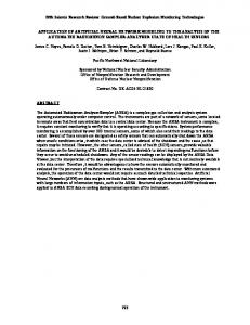
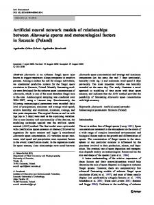
being selected (1/n, n being the number of the available calibration data points). This procedure continues until there are n data points in each bootstrap data set. These bootstrapped data sets were then used to train the ANN for 2000 times and the corresponding sets of weights were computed. Combining each testing input data set with the bootstrapped sets of weights, the ANN yields 2000 bootstrap outputs besides the original. The values are sorted in ascending order and the upper and lower value for a specific confidence level can be found. For example if the nominal coverage is 95% (α = 0.025) the lower value would be the value that lies in the sorted list at the place (a B) = (0.025 2000) = 50. Likewise the upper value of the confidence interval would be the 1950th sorted in ascending order value. The probability of an observed (measured) value to be within the confidence intervals was subsequently evaluated for every calibration and testing data set. According to the available literature the actual coverage of a confidence procedure is rarely equal to the desired (nominal) one, and often is substantially different (Efron and Tibshirani, 1993). It is important to note that if the ANN’s structure has generic errors and is unable to describe specific patterns, the confidence intervals do not account for such errors. 3 RESULTS – DISCUSSION Karstic aquifer simulation is a complex task because the water runs through a dense grid of, practically impossible to map, fractures and fissures with high velocities and flow has open channel characteristics, unlike porous aquifers where the seepage velocities are relatively low and the flow obeys Darcy’s law. The response of a karstic aquifer to rainfall and pumping is very rapid, with what appears to be sudden rises and drops in water table level time series. The utilized ANN model is used to predict groundwater level fluctuation at a well located in a karstic aquifer. It is a classic fully connected multilayer perceptron, trained in a supervised manner with the error back-propagation algorithm. Two hidden layers are used and the number of nodes in each one of the hidden layers was the outcome of a previous optimization procedure, using a DE algorithm (Trichakis et al., 2009). It should be noted that if a second hidden layer is introduced, the local features of the fitting function are extracted in the first hidden layer and the global features are extracted in the second hidden layer (Chester, 1990; Funahashi, 1989; Haykin, 1998). The activation function is the commonly used logistic function, while the synaptic weights are determined in the training procedure through successive weight adaptations. The input parameters consisted of day number, temperature, precipitation at 3 nearby stations, pumping of 16 wells in the region and hydraulic head of the previous day at the two observation wells. The output parameters were the hydraulic head change at the observation well. Available data for 419 days were divided to calibration (training and evaluation) and testing data sets. 3.1 95% confidence intervals The initial thought of this study was the creation of confidence intervals with 95% certainty level. For every data point of both calibration and testing data sets, the percentile intervals were calculated and they are shown in Figure 1 for the two wells. The actual coverage compared to the nominal for the calibration and testing data sets of each observation well is presented in Table 1. The actual coverage was not quite as high as the nominal and this can be attributed to the outliers as a first remark. In order to have an impression of how the coverage would be without the outliers the number of outliers and the number of points that were supposed to be left out are also presented in Table 1. For each well the coverage was recalculated omitting the outliers. This is not scientifically sound as the outliers were present during calibration and have influenced the results but it is just an indication that the low actual coverage values can be attributed to them. As it has been explained in a previous work (Trichakis et al., 2009), these outliers are due to pumping near the observation well 1 and probably to the lack of data for a specific extreme rainfall event that has influenced a rise of the hydraulic head at data points 263–270. The results of both wells show that the testing data sets actual coverage is closer to the nominal one. This could be explained as the calibration period (data points 1–335) has more outliers than the testing period (data points 336–419). The imported uncertainty due to the model’s inherent inability to describe some of the observed data, regardless of the neural weights, cannot be incorporated in 693

Figure 1. Observed, simulated values and bootstrap percentile confidence intervals for 95% certainty level (shown as black error bars) of hydraulic head change for the two wells. Table 1. Actual coverage of the bootstrap percentile intervals, number of points that should theoretically be left out, number of outliers and corrected coverage for wells 1 & 2 with 95% certainty level. Well 1 Data set Actual Coverage Points to be left out theoretically Number of outliers Coverage without outliers

Calibration 79% 17 45 92%

Well 2 Testing 89% 4 7 98%

Full 81% 21 52 93%

Calibration 79% 17 27 87%

Testing 95% 4 0 95%

Full 83% 21 27 89%

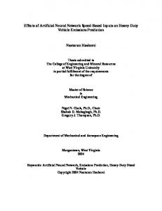
the bootstrap confidence intervals. Nevertheless, as effort is made to create more reliable models with minimal error, the limitations of bootstrap will not be a concern for the researcher that does not need the accuracy of a theoretical statistician. Of course the first concern for all researchers in the field of hydrology should be the creation of better models i.e. models which represent the natural system as accurately as possible. The quantification of the model uncertainty will always be a secondary task and further improvement of such methods would not have any significance to a decision maker if the initial model is not adequate enough. 3.2 Actual coverage for different nominal certainty levels After the first results that suggested the actual coverage was less than the nominal for certainty level 95%, it seemed interesting to see how well bootstrap confidence intervals were estimated for different certainty levels. The confidence intervals and their success rate for different degrees of nominal certainty levels were computed; the actual coverage, separately for calibration and testing data sets, was calculated and the results for the two wells are presented in Figure 2. For the first well the calibration data set demonstrates high agreement between nominal and predicted coverage when it comes to small values of theoretical coverage and up until a level of 694

Figure 2. Theoretical and actual bootstrap percentile confidence intervals coverage for different certainty levels for the calibration and testing data sets of the two wells.

65%; for this range the bootstrap percentile intervals seem adequate enough to quantify the ANN model uncertainty. Unfortunately for higher values of theoretical coverage the results were not equally satisfactory. This can be attributed to the presence of outliers that exist in the initial data and which cannot be modeled with the ANN model. The testing data set for the first well contains much fewer outliers than the calibration set, which is the main reason for the increased actual coverage for small theoretical coverage values. The picture changes at larger confidence levels when the few outliers of the testing data set affect the success of the bootstrap percentile intervals. For example for 95% certainty level the points that should have been left out of the confidence intervals were 4. This was almost impossible to achieve since there were 7 outliers in the testing data set. The second well has a slightly different response. The observed data are far smoother than those of the first well and this is reflected to the smaller length of the confidence intervals. On the other hand, because of the small intervals especially at low confidence levels, the difference between nominal and actual coverage is larger than the first well’s. The results of the testing data set, where there are no outliers, showed that they are extremely close to the nominal. This is the strongest indication that if the model is able to describe the physical system and there are no observed values that the model is absolutely unable to simulate, the bootstrap percentile intervals can quantify the uncertainty quite well, regardless of the nominal confidence level. 4 CONCLUSIONS In hydrological modeling it is important to try and quantify the uncertainty. For ANN models, which have recently found many applications in surface and groundwater hydrology, this can be rather challenging. A first attempt that can be easily modeled is the use of bootstrap methods, and more specifically bootstrap percentile intervals as those were proposed by Efron & Tibshirani (1993). This methodology, though requiring many computations of the ANN model weights (trainings) and is time consuming, can be fully automated. The percentile intervals for 95% confidence level were narrower for the second well, because of the smoother observed values. If the model was able to predict and simulate the extreme points that exist in the observed time series, the actual coverage of the percentile intervals would be closer to the theoretical. This is supported by the fact that the data set that was better simulated by the model and didn’t contain outliers (i.e. the testing data set of the second well) demonstrated increased agreement between actual and nominal coverage. Therefore, when the model is adequate for describing the physical model, the bootstrap percentile intervals can be used to provide a measure of the uncertainty, at least as a first estimation. More sophisticated bootstrap confidence intervals such as bias corrected and accelerated can be utilized if more accuracy is needed. Nevertheless, when the model is unable to accurately simulate specific 695

values regardless of the calibration results (there are outliers in the data set), these values affect the actual coverage of the bootstrap intervals and can lead to over- or underestimation of the correct interval. REFERENCES Babu, G.J. & Feigelson, E. 1996. Astrostatistics. New York: Chapman & Hall. Beven, K. 2008. On doing better hydrological science. Hydrological Processes 22: 3549–3553. Brey, T. 1990. Confidence limits for secondary prediction estimates: Application of the bootstrap to the increment summation method. Mar. Biol. 106: 503–508. Chernick, M.R. (ed. 2) 2008. Bootstrap Methods: A Guide for Practitioners and Researchers. Hoboken, New Jersey: John Wiley & Sons. Chester, D.L. 1990. Why two hidden layers are better than one. International Joint Conference on Neural Networks, Washington DC: 265–268. Coppola, E.A., Rana, A.J., Poulton, M.M., Szidarovszky, F. & Uhl, V.W. 2005. A neural network model for predicting aquifer water level elevations. Ground Water 43(2): 231–241. Diaconis, P. & Efron, B. 1983. Computer-intensive methods in statistics. Scien. American 248: 116–130. Efron, B. & Tibshirani, R. 1993. An Introduction to the Bootstrap. New York: Chapman & Hall. Efron, B. 1988. Bootstrap confidence intervals. Good or bad? Psycol. Bull. 104: 293–296. Funahashi, K.I. 1989. On the approximate realization of continuous mappings by neural networks. Neural Networks 2: 183–192. Haykin, S. (ed. 2) 1998. Neural Networks: A Comprehensive Foundation. New Jersey: Prentice Hall. Jia, Y. & Culver, T.B. 2006. Bootstrapped artificial neural networks for synthetic flow generation with a small data sample. Journal of Hydrology 331(3–4): 580–590. Lallahem, S. & Mania, J. 2003. A nonlinear rainfall-runoff model using neural network technique: example in fractured porous media. Mathematical & Computer Modelling 37(9–10): 1047–1061. Lallahem, S., Mania, J., Hani, A. & Najjar, Y. 2005. On the use of neural networks to evaluate groundwater levels in fractured media. Journal of Hydrology 307(1–4): 92–111. Maier, H.R. & Dandy, G.C. 2000. Neural networks for the prediction and forecasting of water resources variables: a review of modelling issues and applications, Environmental Modelling & Software 15(1): 101–124. Nayak, P., Rao, Y. & Sudheer, K. 2006. Groundwater Level Forecasting in a Shallow Aquifer Using Artificial Neural Network Approach. Water Resources Management 20(1): 77–90. Paas, G. 1994. Assessing predictive accuracy by the bootstrap algorithm. In M. Marinaro & P.G. Morasso (eds) Artificial Neural Networks, ICANN ’94; Proc. intern. conf. 2: 823–826. Parmanto, B., Munro, P.W., & Doyle, H.R. 1996. Improving committee diagnosis with resampling techniques. In D.S. Touretzky, M.C. Mozer, & M.E. Hasselmo (eds), Advances in Neural Information Processing Systems; Proc. conf., 1995 8: 882–888. Todini, E. & Mantovan, P. 2007. Comment on: ‘On undermining the science’ by Keith Beven, Hydrological Processes 21: 1633–1638. Tourassi, G.D., Floyd, C.E., Sostman, H.D., & Coleman, R.E. 1995. Performance evaluation of an artificial neural network for the diagnosis of acute pulmonary embolism using the cross-validation, jackknife, and bootstrap methods. WCNN ’95 2, 897–900. Trichakis, I.C., Nikolos, I.K. & Karatzas, G.P. 2009. Optimal selection of artificial neural network parameters. Hydrological Processes. 23: 2956–2969. Ueda, N., & Nakano, R. 1995. Estimating expected error rates of neural network classifiers in small sample size situations: A comparison of cross-validation and bootstrap. 1995 IEEE Neural Networks, Proc. Intern. Conf. 1, 101–104. Wahrendorf, J. & Brown, C.C. 1980. Bootstrapping a basic inequality in the analysis of joint action of two drugs. Biometrics 36: 653–657.

696