numerical model, bar forrmition, large wave tank, .odes seawall, beach fill ... Station, Vicksburg, Mississippi, and in part at the Department of. Water Resources ...
INSTITUTIONEN FOR TE KNISK VATTENRESURSLARA I 'JNDS UNIVERSITET, TEKNISKA OCH NATURVETENSKAPLIGA HOGSKOLAN LUND UNIVERSITY, INSTITUTE OF SCIENCE AND TECHNOLOGY
8
QUANTIFICATION OF BEACH PROFILE CHANGE by
Ln
Magnus Larson
mf
OTIC
co
Lund, Sweden, 1988 Apprvo~d
foT
Mtt~1huo
public r.Aem; LUnIjted
CODEN: LUTVDG / (TVVR - 1008) / I - 293 (1988)
QUANTIFICATION OF BEACH PROFILE CHANGE
by
Magniiq Larson
DTIC /.ELECTE0 MAY ! 9 1988 D
H DLUMUTION STATEMENT A Approved for public ro3.u. Distribution Unlimited
8 v
07 005
ABSTRACT
An engineering numerical model is presented for simulating beach profile change in the surf zone produced by wave-induced crossshore sand transport. The model simulates
the dynamics of
macroscale profile change, such as growth and movement of breakpoint h-rs and berms.
The foundation for the development of the numerical model was two large wave tank experiments consisting altogether of 42 cases with different incident wave conditions, median grain size, and initial beach shape. An extensive analysis was made to define and quantify parameters describing profile change and relate these parameters to wave and sand characteristics.
The model was developed using transport rate relationships inferred from profile change measured in the
1
rg
wave tanks.
Distributions of the net transport rate were obtained by integrating the sand conservation equation across pairs of profiles separated in time. Semi-empirical transport rate relationships were developed for different regions of the profile.
The beach profile change model was calibrated and verified with the prototype-scale laboratory data. The model was also applied to simulate field beach profile change measured in five storm events and good agreement was found. Beach profile evolution in the vicinity of a seawall and the adjustment of a beach fill to incident waves were other cases studied with the model.
Keywords:
Beach profile change, cross-shore sand transport, numerical model, bar forrmition, large wave tank,
seawall, beach fill
.odes Avall and/or Special
PREFACE
This study was conducted in part at the Coastal Engineering Research Center (CERC), U.S. Army Engineer Waterways Experiment Station, Vicksburg, Mississippi, and in part at the Department of Water Resources Engineering, Institute of Science and Technology, University of Lund, Lund, Sweden. The work at the University of Lund was performed under the supervision of Professor Dr. Gunnar Lindh, Department of Water Resources Engineering, whereas the portion of the study performed at CERC was under the supervision of Dr. Nicholas C. Kraus, Senior Research Scientist, Research Division. The study at CERC wi
conducted from 23 June
19R6 through 31
July 1987 under the work unit Surf Zone Sediment Transport Processes, Shore Protection and Restoration Program.
The work
was funded through the U.S. Army Research, Development and Standardization Group, UK, under contract No. DAJA-86-C-0046. The CERC portion of the investigation was under the general direction of Dr. James R. Houston, Chief, CERC; Mr. H. Lee Butler, Chief, Research Division (CR),
CERC.
The following is a list of technical articles written as an outcome of this investigation.
These articles constitute
to a
varying degree the foundation of the work contained herein and were written simultaneously with this thesis. are
Accordingly, most
in the process of being published.
Larson, M., Morphology,"
Larson, M.,
and Kraus, N. C.
1988a.
1:
submitted for publication.
and Kraus, N. C.
1988b.
Net Cross-Zhore Snd S Tranprt
Larson, M.,
"Beach Profile Charge,
and Kraus, N. C.
Numerical Model,"
,
1988c.
"Beach Profile Change, 2: ti
"Beach Profile Change, 3:
submitted for publication. 1
for publication.
Larson, M.,
Kraus, N. C.,
and Sunamura, T.
1988.
"Beach Profile
Change: Morphology, Transport Rate, and Numerical Simulation," Proceedings of the 21th Coastal Engineering Conference, kmcrican Society of Civil Engineers, in preparation.
Kraus, N. C.,
and Larson, M.
1988a.
"Beach Profile Change
Measured in the Tank for Large Waves, 1956-1957 and 1962," Technical Report CERC-88-O0
, Coast,,I
Engineering Research
Center, U.S. Army Engineer Waterways Experiment Station, Vicksburg, MS, in press.
Kraus, N. C.,
and Larson, M.
1988b.
"Prediction of Initial
Profile Adjustment of Nourished Beaches to Wave Action,"
Proceed-
ings of Beach Preservation Technology '88, American Shore and Beach Preservation Association, in press.
2
ACKNOWLEDGEMENTS
First of all I would like to express my sincere appreciation to Dr. Nicholas C. Kraus, CoasLal Engineering Research Center (CERC), for the guidance and support provided by him during this thesis work.
Without his untiring dedication, the successful
completion of this investigation would not have been possible. I would like to thank my advisor, Professor Dr. Gunnar Lindh, for supervising the thesis work and Dr. Hans Hanson for introducing me to the field of coastal engineering and providing valuable comments in the review of this thesis. Furthermore, I would like
to acknowledge Mr. Ronny Berndtsson, Dr. William
Hogland, and Dr. Lennart J6nsson, with whom I worked together in various projects prior to my thesis studies and who decisively influenced my professional attitude. I also wish to thank Mr. Bruce A. Ebersole, CERC, for valuable discussions regarding breaker decay models, and Mr. Mark B. Gravens, CERC, for extending my knowledge of the English language and his kind help in many matters, both professional and private.
Ms. Jane M. Smith, CERC, provided the small-scale
laboratory data on breaking waves and the data from the CERC Field Research Facility, which was greatly appreciated. special thanks
A
to Mr. John Brandon and Ms. Lucy W. Chou, who
carried out most of the tedious work converting the Japanese data into computer format.
Also, I would like to express my sincere
thanks to all other co-workers at CERC who made my stay in Vicksburg a pleasant and successful one. Furthermore, I would like
to thank Professor Dr. Tsuguo
Sunamura, University of Tsukuba, Japan, whose great insight in the physics of beach profile change inspired many aspects of this study. The U.S. Army Research, Development, and Standardization
3
Group, London, is gratefully acknowledged for funding this project and making my stay at CERC possible. Finally, I wish to thank Mrs. Kinuyo Kraus for the incredible amount of work she did, preparing all the figures for this report.
Lund, March, 1988.
Magnus Larson
4
CONTENTS
PREFACE.......................................................
Page 1I
ACKNOWLEDGEMENTS.............................................
3
LIST OF FIGURES..............................................
8
LIST OF TABLES...............................................15s PART I:
INTRODUCTION.....................................
Problem Statement and Objectives...................... Procedure Used......................................... Basic Terminology..................................... Profile morphology............................... Nearshore waves.................................. PART II:
16 16 18 20 22 23
LITERATURE REVIEW................................
25
Literature........................... ................. Synthesis of Previous Work............................
25 50
PART III:
DATA EMPLOYED IN THIS STUDY......................
Introduction........................................... Small-scale laboratory approach.................. Field approach................................... Prototype-scale laboratory approach ............... Data Employed in This Study........................... Data base......................................... CE experiments................................... CRIEPI experiments............................... Field data........................................ Summary........................................... PART IV:
54 54 54 55 56 57 57 58 61 63 65
QUANTIFICATION OF MORPHOLOGIC FEATURES ............
66
Data Analysis Procedure............................... Concept of Equilibrium Beach Profile.................. Criterion for Distinguishing Profile Response .... Bar and berm..................................... Shoreline movement............................... Application to small-scale data.................. Form and Movement of Bars............................. Bar genesis....................................... Equilibrium bar volume........................... Depth to bar crest .................................
66 70 73 73 82 84 86 86 90 94
5
Ratio of trough depth to crest depth .......... Maximum bar height ............................... Bar location and speed of movement ............ Distance from break point to trough bottom .... Bar slopes ....................................... Step and terrace slope ........................... Form and Movement of Berms ......................... Berm genesis ..................................... Active profile height ............................ Equilibrium berm volume .......................... Maximum berm height .............................. Berm slopes ...................................... Summary and Discussion of Morphologic Features ..... PART V:
97 99 104 107 i 115 116 116 119 120 122 124 125
CROSS-SHORE TRANSPORT RATE......................
129
Introduction .......................................... General Features of Cross-Shore Transport .......... Classification of Transport Rate Distributions ..... Approach to Equilibrium............................... Peak otfshore transport .......................... Peak onshore transport ........................... Magnitude of Net Cross-Shore Transport Rate ........ Transport Regions ..................................... Zone I: Net transport rate seaward of the break point ...................................... Zone II: Net transport rate between break point and plunge point ........................... Zone III: Net transport rate in broken waves ............................................. Zone IV: Net transport rate on the foreshore ........................................ Summary and Discussion of Net Transport Rate .......
129 132 135 143 144 148 151 153
Part VI:
NUMERICAL MODEL OF BEACH PROFILE CHANGE .......
Introduction .......................................... Methodology ............................................ Wave Model ............................................. Breaking criterion and breaker height ......... Breaker decay model .............................. Transport Rate Equations .............................. Profile Change Model .................................. Calibration and Verification of Numerical Model .... Summary and Discussion of Numerical Model .......... PART VII:
APPLICATIONS OF THE NUMERICAL MODEL ...........
Introduction .......................................... Sensitivity Analysis of Model Parameters ........... 6
154 161 163 169 171 173 173 174 176 177 182 186 194 198 204 207 207 207
Influence of K ................................... Influence of e................................... Influence of wave model parameters ............ Influence of equilibrium energy dissipation ...................................... Influence of wave period and height ........... Influence of runup height ....................... Effect of Time-Varying Water Level and Waves ....... Water level, wave height, and wave period ..... Multiple Barred Profiles .............................. Simulation of Field Profile Change ................... Data set ......................................... Calibration of numerical model with field data ....................................... Results .......................................... Sensitivity tests ................................ Discussion of field simulation ................ Comparison With the Kriebel Model .................... Overview ......................................... Calibration...................................... Comparisons of model simulations .............. Numerical Modeling of Beach Profile Accretion ...... General discussion ............................ Model calculation ..............................
208 210 211 213 215 217 219 221 226 231 233 234 237 241 243 245 245 246 246 250 250 252
Numerical Modeling of the Influence of a Seawall ................................................ Profile with seawall ............................. Profile with seawall and beach fill ........... PART VIII:
SUMMARY AND CONCLUSIONS ..........................
254 254 256 263
REFER ENCES ...............................................
271
APPENDIX A:
291
NOTATION .......................................
7
LIST OF FIGURES No. I
2
3
4
5
6
7
8
Definition sketch of the beach profile: (a) morphology, and (b) nearshore wave dynamics (after Shore Protection Manual 1984) ................
21
Tank for large waves at Dalecarlia Reservation, Washington DC, where the CE experiments were conducted in 1956-57 and 1962 .......................
59
View of the wave generator in the tank for large w av es . .. ... .. .. .. . . ... . ... .. ... .. .. .. ... .. .. .. .
59
Notation sketch for beach profile morphology: (a) bar profile, and (b) berm profile ...........
68
Absolute sum of profile change as a function of time for selected CE and CRIEPI cases ...........
71
Criterion for distinguishing bar and berm profiles by use of wave steepness and dinensionless fall velocity ............................................
77
Criterion for distinguishing bar and berm profiles by use of wave steepness and ratio of wave height to grain size ...............................
78
Criterion for distinguishing bar and berm
profiles
by use of wave steepness and fall velocity parameter ........................................... 9
10
11
12
79
Criterion for distinguishing bar and berm profiles by use of ratio of breaking wave height and grain size, and Ursell number at breaking .......
81
Criterion for distinguishing shoreline retreat and advance by use of wave steepness, dimensionless fall velocity, and initial beach slope ..........
83
Criterion for distinguishing bar and berm profiles applied to small-scale laboratory data by use of wave steepness and (a) dimensionless fall velocity, and (b) ratio of wave leight to grain size ................................................
85
Growth and movement of breakpoint lar with elapsed time and location of break point ....................
88
8
13
14
15
16
17
18
19
20
21
22
23
24
25
26
27
Beach profile from CRIEPI Case 6-2 measured after 4.2 hr of wave action together with the initial profile and the wave height distribution across-shore ........................................
89
Growth of bar -,olume with elapsed time: (a) CE data, and (b) CRIEPI data ..........................
91
Comparison of measured equilibrium bar volume Vm and empirical prediction Vp ..................
94
Depth to bar crest as a function of elapsed time: (a) CE data, and (b) CRIEPI ........................
96
Relationship becween depth to bar crest hc and breaking wave height Hb ............................
97
Ratio of depth to trough bottom and depth to bar crest ht/hc as a function of wave period ........
99
Maximum bar height as a function of time elapsed: (a) CE data, and (b) CRIEPI data ................
101
Comparison of measured equilibrium bar height (ZB)m and empirical prediction (ZB)p ............
103
Horizontal movement of bar center of mass with elapsed time: (a) CE data, and (b) CRIEPI data ................................................
105
Speed of bar movement with elapsed time: (a) CE data, bar center of mass; (b) CE data, bar crest; (c) CRIEPI data, bar center of mass; and (d) CRIEPI data, bar crest .........................
108 109
Comparison of measured and predicted nondimensional horizontal distance between break point and trough bottom ............................
i1
Shoreward slope of main breakpoint bars as a function of elapsed tiie ...........................
113
Seaward slcpes of main breakpoint bars as a function of elapsed time ...........................
114
Time evolution of representative step and terrace slopes ..............................................
117
Relation between berm center of mass and wave runup ...............................................
119
9
28
29
30
31
32
33
34
35
36
37
38
39
40
Growth of berm volume with elapsed time: (a) CE data, and (b) CRIEPI data .......................
121
(;rowth of maximum herin height (a) CE data, and (b) CRIEPI
12
with elapsed data ...................
time:
Growth of representative berm slopes with elapsed t i me . . . . . . . . . . . . . . . . . . . . . . . . . . . . . . . . . . . . . . . . . . . .
125
Evolution of beach profile under constant incident wave conditions for an erosional case (C a se 30 0 ) . ... .. .. .. . .. .. .. .. . .. .. .. .. .. .. .. ....
13 3
Calculated distributions of net cross-shore sand transport rate for an erosional case (C a se 30 0 ) . ... .. .. .. ... ... .. .. ... .. .. .. ... .. .. ..
134
Evolution of beach profile under constant incident wave conditions for an accretionary case (C a se 101 ) . ... .. .. .. ... ... .. .. ... .. ... .. .. .. ... .
136
Calculated distributions of net cross-shore sand transport rate for an accretionary case (C a se 10 1) . ... .. .. ... .. ... .. .. ... .. ... .. .. .. .. ..
13 7
Classification of net cross-shore sand transport rate distributions: (a) Type E, Erosional: (b) Type A, Accretionary; and (c) Type AE, Mixed Accretionarv and Erosional ......................
13q
Evolution of beach profile under constant incident wave conditions for a mixed accretionary and erosional case (Case 3-2) .......................
141
Decay of average absolute net cross-shore sand transport rate: (a) CE data, 16 cases; and (b) CRIEPI data, 17 cases .......................
145
Evolution of peak offshore net sand transport rate with time for 16 CE cases .......................
146
Decay of peak offshore sand transport rate with time for Case 300, and a best-fit empirical predictive expression ...........................
147
Evolution of peak onshore net sand transport rate with time for 16 CE cases .......................
144)
10
41
42
Decay of peak onshore sand transport rate with time for Case 101, and a best-fit empirical predictive equation ................................ DefiniLion sketch for four principal zones of cross-shore sand transport .........................
43
44
45
46
47
48
49
50
51
52
53
54
150
152
Time-behavior of spatial decay rate coefficient for the zone seaward of the break point .........
156
Comparison of net offshore sand transport rates at different times seaward of the break point and an empirical predictive expression ..........
157
Comparison of spatial decay rate coefficients and an empirical predictive expression ..........
159
Comparison of net onshore sand transport rates at different times seaward of the break point and an empirical predictive equation ............
160
Net cross-shore sand transport rate distributions between break point and plunge point ............
163
Net cross-shore sand transport rate versus calculated wave energy dissipation per unit volume in broken wave region ......................
166
Time behavior of net cross-shore sand transport rate distribution on the foreshore ..............
170
Distribution of breaker ratio for the CRIEPI data................................................
178
Distribution of breaker ratio for small-scale laboratory data ....................................
178
Comparison between measured breaker ratio and predicted breaker ratio from an empirical relationship based on beach slope seaward of the break point and deepwater wave steepness ........
180
Ratio between breaking and deepwater wave height as a function of deepwater wave steepness .......
181
Measured wave height distributions across the surf zone for Case 3-4 and corresponding wave heights calculated with a breaker decay model ...........
184
11
Definition sketch for describing avalanching along the profile .........................................
194
56
Calibration of numerical model against Case 6-1...
201
57
Net cross-shore transport rates at selected times for Case 6-1 ........................................
202
Total sum of squares of the difference between measured profile and simulated profile with the numerical model for all profile surveys and all cases in the calibration ...........................
204
Verification of numerical model against: (a) Case 400, and (b) Case 6-2 ..............................
205
Evolution in time of bar volume for different values of transport rate coefficient ............
209
Evolution in time of maximum bar height for different values of transport rate coefficient..
209
Evolution in time of bar volume for different values of slope coefficient in the transport equation ............................................
210
Evolution in time of bar volume for different values of wave decay coefficient ................
211
Evolution in time of bar volume for different values of stable wave height coefficient ........
214
Evolution in time of bar volume for different values of median grain size ........................
214
Movement of bar mass center as a function of time for different values of median grain size .......
216
Evolution in time of bar volume for different values of wave period ..............................
217
Evolution in time of bar volume for different values of runup height .............................
218
Verification of numerical model against Case 911 having a varying water level with time ..........
220
55
58
59
60
61
62
63
64
65
66
67
68
69
12
70
71
72
73
74
75
76
77
78
79
2
Numerical simulation of hypothetical case with sinusoidally varying wave period between 6 and 10 sec, and constant wave height and water level ...............................................
221
Numerical simulation of hypothetical case with sinusoidally varying water level between -1.0 and 1.0 m, and constant wave height and period ..............................................
222
Numerical simulation of hypothetical case with sinusoidally varying wave height between 1.0 and 3.0 n, and constant wave period and water level ...............................................
223
Transport rate distributions at selected times for case with sinusoidally varying wave height ......
224
Numerical simulation of hypothetical case with sinusoidally varying wave height between 1.0 and 3.0 m, water level varying between -1.0 and 1.0 m, and constant wave period ...................
225
Calibration of numerical model against Case 500, reproducing the second breakpoint bar ...........
229
Distribution of sediment grain sizes across profile line 188 at Duck, North Carolina (after 1Iowd and Birkemeier 1987) ..........................
232
Calibration of numerical model against field data from profile line 188 at Duck for event (840403-840406). Variation with time of: (a) wave height, wave period, and water level; and (b) simulation result ..........................
238
Verification of numerical model against field data from profile line 188 at Duck for event (821207-821215). Variation with time of: (a) wave height, wave period, and water level; and, (b) simulation result .........................
240
Prediction of numerical model against field data from profile line 188 at Duck for verification event (821207-821215) omitting water level variation ..........................................
242
13
80
81
82
83
84
85
86
87
88
Prediction of numerical model against field data from profile line 188 at Duck for verification event (821207-821215) omitting variation in wave height, wave period, and water level ............
243
Simulation of hypothetical case with sinusoidally varying water level with present model and Kriebel model: (a) full beach profile, and (b) detail of dune .....................................
24]
Simulation of hypothetical case with step-increase in water level with present model and Kriebel (a) full beach profile, and (b) detail model: of dune .............................................
249
Calibration of numerical model against Case 101 showing berm build-up ..............................
253
Simulation of hypothetical case with and without seawall located on the foreshore ..................
255
Wave height and water level as a function of elapsed time used in beach fill simulations .....
257
Beach profiles at selected times for hypothetical storm event and original beach without fill: grain size (a) 0.25 mm, and (b) 0.40 mm .........
258
Beach profiles at selected times for hypothetical storm event and beach with berm fill: grain size (a) 0.25 mm, and (b) 0.40 mm ......................
260
Beach profiles at selected times for hypothetical storm event and beach with Bruun fill: grain size (a) 0.25 mm, and (b) 0.40 mm ...............
261
14
LIST OF TABLES No. 1
2
Wave Height, Wave Period, and CE Experiments: Water Depth in the Horizontal Section of the Tank, and Deepwater Wave Steepness ............. Wave Height, Wave Period, CRIEPI Experiments: the Horizontal Section of in and Water Depth Slope, and Deepwater Beach Initial Tank, the Wave Steepness .................................
62
64
3
Selected Criteria for Classifying Bar and Berm Profiles ...........................................
4
CE Experiments:
Values of Selected Quantities...
127
5
Values of Selected CRIEPI Experiments: Quantities ........... .........................
128
15
76
QUANTIFICATION OF BEACH PROFILE CHANGE
PART I:
INTRODUCTION
Problem Statement and Objectives
The study of beach profile change in the broad sense encompasses nearshore processes that shape the beach on all spatial and temporal scales.
Beach profile changc
is a phenome-
non of fundamental interest and, as such, has been studied bv geologists, oceanographers, and coastal engineers. In coastal engineering, quantitative understanding of beach profile change is pursued mainly to allow prediction of beach evolution in the vicinity of planned or existing engineering projects.
Two types of coastal engineering problems of par-
ticular importance for which predictive
tools are needed are
beach and dune erosion that occurs under storm waves and high water levels, and adjustment of beach fill to long-term wave action.
The time scale associated with storm-induced erosion is
on the order of 1 to 3 days and depends on the level and duration of the storm surge as well as the waves, whereas the time scale of beach fill adjustment is several weeks to several months and depends on season of placement,
fill material, and wave climate
at the coast. It is often convenient to separate nearshore sediment movement into two components, longshore sediment transport and cross-shore sediment transport, although this separation is not always valid in a strict sense.
Longshore sediment transport
figures prominently in situations involving loss of sediment supply, such of damming of rivers, and in impoundment at structures such as groins and jetties. 16
In these cases
longshore
transport is the major process governing nearshore topography change and cannot be neglected. For beaches located away from structures, mouths,
inlets, and river
it may be appropriate to neglect longshore transport as a
first approximation, i.e.,
assume the gradient of the longshore
transport rate is negligibly small at the site.
In this case,
cross-shore transport will determine the change in beach profile contours.
This assumption will be made in this investigation:
longshore sediment transport is neglected and profile change produced solely by cross-shore sediment transport is considered. The ultimate goal of this investigation is development of a numerical model to predict beach profile change produced by wave action. ture;
Numerous such models have been reported in the litera-
however, apart from the present work only one highly
schematized numerical model has been considered sufficiently accurate to be of engineering use.
Most efforts appear to have
failed because the level of detail attempted was beyond the state of knowledge of the physical processes involved.
At present,
knowledge is very limited on the collective motion of sediment particles in spatially varying flows of oscillatory currents, wave-induced mean current, and turbulence fields of breaking waves.
Numerous other complicating factors, such as the complex
fluid motion over an irregular bottom, and absence of rigorous descriptions of broken waves and sediment-sediment interaction, also make the problem of computing sediment transport and resultant beach profile change essentially impossible if a firstprinciples approach at the microscale
is taken.
On the other hand, despite the incredibly complex and diverse processes and factors involved, beach profile change if viewed on the macroscale is remarkably smooth and simple. Certain prominent features, such as bars, troughs, and berms go through cycles of formation, growth, movement, and erasure with a morphodynamic pattern that has been reasonably well described by a number of qualitative conceptual models. 17
The question can then
be asked whether it is not possible to develop a quantitative (numerical) model of beach profile change based on empirically determined global relations for the wave-induced net cross-shore sediment (sand) transport rate that can be inferred from the smooth and regular change observed to occur during beach profile evolution.
Development of such a model is the subject of this
investigation.
Procedure Used
The principal physical mechanisms which decermine beach profile change must be quanLitatively described to model the profile response numerically.
For this purpose it
is necessary
to study profile evolution under varying waves, sand characteristics,
and profile shape.
However, to establish cause and effect
relationships between the governing factors and the profile response, it must be possible to clearly delineate these relationships.
Laboratory facilities provide an environment where
such investigations may be carried out efficiently, while allowing for data sampling at almost any spatial or temporal scale.
The difficult problem of transforming observations made
under scale distortion is eliminated if experiments are performed at the scale of the prototype, i.e.,
at a sufficiently large
scale as to satisfactorily represent the interaction between fluid forces and sand grains that produces significant sand transport in the field. Use of field profile data as a basis for developing a numerical model is extremely difficult due to the complexity and randomness of naturally occurring conditions and cost of data collection.
Ultimately a numerical model must be verified
against field data but in the process of development of the model laboratory data can provide considerably more insight into the relative influence of the factors producing the profile change. 18
Study of these individual factors implicitly assumes the validity of the superposition principle for application of the model the general case.
to
For example, examination of the effect of
water level variation on profile evolution under fixed incident waves isolates the influence of this factor and allows understanding of the related physical processes
involved.
A combina-
tion of such observations constitute the foundation for a numerical model which is used in a predictive mode for varying water level and wave conditions, even though these factors have been evaluated separately.
Consequently, careful data analysis
is the basis for many assumptions and empirical relationships employed in the numerical model developed here and the first logical step towards understanding beach profile change by this procedure. From an engineering point of view it is of considerable importance to quantify properties related to beach profile change.
This regards both geometric parameters such as bar
volume and depth to bar crest, as well as more complex quantities such as net cross-shore sand transport rates.
Any structure or
activity extending into the nearshore region is influenced by and influences the evolution of the beach profile,
thus requiring
quantitative estimates of profile change under various environmental and design conditions.
A thorough analysis of different
geometric characteristics of the profile and their dependence on the wave and sand properties is in this respect valuable. Through this analysis the important processes shaping the beach and generating different morphologic features may be clarified, forming the conceptual framework for a numerical model. A fundamental assumption of this study is that beach profile change is mainly governed by breaking of short-period waves the approximate range of 3-20 sec).
(in
No attempt has been made to
include the effect of long-period waves, such as partially standing waves or infragravity waves, regarding profile evolution, as no adequate data on profile change are available that 19
permit firm conclusions to be made. have indicated that, in some cases, wave energy can be
Recent field investigations infragravity or long-period
larger near the shoreline than that of the
existing short-period waves.
This dominance of the wave energy
spectrum in very shallow water by long-period waves is expected to play an important role in beach profile processes on the shore face and, possibly, the inner surf zone.
However, no relation-
ship between beach profile change and infragravity waves exists at present due to lack of data.
When such data become available,
superposition should allow calculation of profile change under both short- and long-period waves. The main purpose of the data analysis is not to derive widely applicable relationships for geometric properties of the profile, but to identify the important factors governing profile change.
These factors will be integral parts in the conceptual
foundation underlying the numerical model development.
In some
cases however, empirical relationships derived from the data are used directly in the model if general conclusions about the behavior of the quantity can be made.
Basic Terminology
Nomenclature associated with the beach profile and nearshore region is presented which is used throughout the report. defined in the Shore Protection Manual adapted to a large extent.
Terms
(SPM 1984) have been
However, for some quantities a
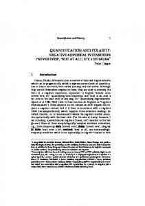
slightly different description is employed that is better suited for nearshore processes as related to beach profile change. Figures la and lb are definition sketches pertaining to beach profile morphology and nearshore wave dynamics, respectively. The portion of the beach profile of interest here spans acrossshore from the dunes
to the seaward end of the nearshore zone.
20
A COASTAL AREA
I
NEARSHORE ZONE
BEACH OR SHORE
COAST-,
UNE~~B
FOEHR
TROUGH LEVEL
H %L
HpUH- A\ATEFH
L" L
LOW '.ATER LEVEL
OFFSHORE ZONE
ZONE
i OcSURF
xI BROKEN WA VES
Cc
01I
ULINNER t
BREAKERS RE-FORMED WASTP RUNUP
BACIKRUSH
OUTER BREAKERS LL-WA TER LEVEL
RAE-PT
OUTER BAR
DEEP BAR
BP BREAK POINT PP PLUNGE POINT RP REFORMATION POINT
Figure 1.
Definition sketch of the beach profile:
(a)
morphology, and (b) nearshore wave dynamics (after Shore Protection Manual 1984) 21
Profile morphology
As waves approach the beach from deep water they enter the nearshore zone.
The seaward boundary of the nearshore zone is
dynamic and for our purpose is considered to be the depth at which waves begin to shoal upward.
The shoreward boundary of
wave action is also dynamic and is at the limit of wave runup, located at the intersection between the maximum water level and the beach profile.
A gently sloping bottom will cause a gradual
shoaling of the waves, leading to an increase in wave height and finally to breaking at a point where the wave height is about equal to the water depth. denoted as the offshore; i.e.,
The region seaward of wave breaking is the inshore encompasses the surf zone,
that portion of the profile exposed to breaking and broken
waves.
The broken waves propagate with large energy dissipation
through turbulence, initiating and maintaining sand movement.
At
the beach face, the remaining wave energy is expended by a runup bore as water rushes up the profile. The flat area shoreward of the beach face is called the backshore and is only exposed during severe wave conditions or when the water level
is unusually high.
On the backshore one or
several berms may exist, which are accretionary features where material has been deposited by wave action. ary"
The term "accretion-
refers to features generated by sand transport directed
onshore.
A step often develops immediately seaward of a berm
where the slope depends on the properties of the runup bore and the sand grains.
Under storm wave action a scarp may also form;
here, the term "step" will be used to denote both a scarp and a step.
On many beaches a line of dunes is present shoreward of
the backshore which consists of large ridges of unconsolidated sand that have been transported by wind from the backshore. A bar is a depositional feature formed by sand that was transported from neighboring areas.
Several bars may appear
along a beach profile, often having a distinct trough on the 22
shoreward side.
Bars are highly dynamic features that
respond to
the existing wave climate by changing form and translating across-shore, but at the same time bars influence the waves incident upon them.
If a bar was created during an episode of
high waves, it may be located at such great depth that very little or almost no sand transport actiity takes place until another period of high waves occurs.
Some
transport from the bar
caused by shoaling waves may take place, but the time scale of this process is considerably longer than if the bar is located close to the surf zone and breaking or broken waves.
Nearshore waves
The above-discussed terminology is mainly related to the various regions and features of the beach profile.
Nearshore
aves are also described by specialized terminology (Figure lb). Again, some definitions are not unique and describe quantities that change in space and time.
The region between the break
point and the limit of the backrush where broken waves prevail called the surf zone.
is
The swash zone extends approximately from
the limit of the backrush to the maximum point of uprush, coinciding with the beach face. toward shore, shape;
As waves break and propagate
reformation may occur depending on the profile
that is,
the translatory broken wave form r-verts to an
oscillatory wave.
This oscillatory wave will treak again as it
reaches sufficiently shallow water, transforming into a broken wave with considerable energ, dissipation.
The region where
broken waves have reformed to oscillatory waves is called the reformation zone, and the point where this occurs is the wave reformation point. The break point is located where the maximum particle velocity of the wave exceeds the wave celerity and the front face of the wave becomes vertical.
As a wave breaks,
the crest falls
over into the base of the wave accompanied by large amount of 23
energy dissipation. type (Calvin 1972),
If the breaking waves are of the plunging the point of impingement is easily recognized
and denoted as the plunge point.
For spilling breakers, however,
the plunge point concept is not commonly used but such a point could be defined using the location of maximum energy dissipation
This definition is in accordance with the conditions
prevailing at the plunge point for a plunging breaker. A beach profile exposed to constant wave and water level conditions over a sufficiently long time interval will attain a fairly stable shape known as the equilibrium profile.
On a beach
in nature, where complex wave and water level variations exist, an equilibrium profile may never develop or, if so, only for a short time before the waves or water level again change. However, the equilibrium concept remains useful since it provides information of the amount of sand that has to be redistributed within the profile of wave conditions.
to attain the natural shape for a specific The equilibrium profile is in general
considered to be a function of sand and wave characteristics.
24
set
PART II:
LITERATURE REVIEW
From the earliest investigations of beach morphology, the study of profile change has focused to a large extent upon the properties of bars.
A wide range of morphologic features have
been classified as bar formations by different authors, and different terminology is used to denote the same feature.
The
literature on beach profile change is vast, and this chapter is intended to give a chronological survey of results relevant to the present work.
Literature
Many of the first contributions to the study of bars were made by German researchers around the beginning of this century. Lehmann
(1884) noted the role of breaking waves in suspending
sand and found that profile change could occur very rapidly with respect to offshore bar movement.
Otto
(1911) and Hartnack
(1924) measured geometric properties of bars
in the Baltic Sea,
such as depth to bar crest, distance from shoreline to bar crest, and bar slopes.
Hartnack
(1924) pointed out the importance of
breaking waves in the process of bar formation and noted that the distance between bar crests increased with distance from shore for multiple bars and that the depth to bar crest increased correspondingly. Systematic
laboratory modeling of beach profile evolution
appears to have been first applied by Meyer
(1936), who mainly
investigated scaling effects in movable bed experiments.
He also
derived an empirical relationship between beach slope and wave steepness.
Waters
(1939) performed pioneering work on the
characteristic response of the beach profile to wave action, and classified profiles as ordinary or storm type. wave steepness can be used to determine the 25
He concluded that
type of beach profile
that developed under a set of specific wave
conditions.
The
process of sediment
sorting along the profile was demonstrated
the experiments,
which the coarser material
in
plunge point and finer material
in
remained near the
moved offshore.
Bagnold (1940) studied beach profile evolution in smallscale laboratory experiments by use of rather coarse material (0.5-7.0 mm), up.
resulting in
accretionary
He found that foreshore
profiles with berm build-
slope was independent
height and mainly a function of grain size.
of
the wave
However, the
equilibrium height of the berm was linearly related to wave height.
The effect of a seawall on the beach profile was
investigated by allowing waves varying the water level,
to reach the end of the tank.
By
a tide was simulated, and in other
experiments a varying wave height was employed. Evans by Evans) these
(1940)
to be
the result of plunging breakers,
the bar and trough
to form a unit with the
located shoreward of the bar.
and lows
would develop. in
shoreward.
Also,
a change
lie
trough always
If the profile slope was mild so
that several break points appeared,
a change
bal Is
along the eastern shore of Lake Michigan and concluded
features
regarded
studied bars and troughs (named
in
a series of bars
wave conditions
and troughs
could
result
in
bar shape and a migration of the bar seaward or A decreasing water level would cause the
laner-most
bar to migrate onshore and take the form of a subaqueous dune. whereas an increase in water level would allow a new bar system to develop inshore and the m(.st seaward bars would become fossilized. In connection with amphibious World War II,
landing operations during
Keulegan (1945) experimentally obtained simple
relations for predicting depth
to bar crest and trough depth.
found the ratio between trough and crest depths
He
to be approxi-
mately constant and independent of wave steepness.
Important
contributions to the basic understanding of the physics of beach profile change were also made through further laboratory experi26
ments by Keulegan (1948).
The objective of the study was to
determine the shape and characteristics of bars and how they were molded by the incident waves.
He recognized the surf zone as
being the most active area of beach profile change and the breaking waves as the cause of bar formation.
The location of
the maximum sand transport rate, measured by trap, was found to be close to the break point, and the transport rate showed a bood correlation with the wave height envelope.
Keulegan (1948)
noted
three distinct regions along the profile where the transport properties were different from a morphologic perspective.
A
gentler initial beach slope implied a longer time before the equilibrium profile was attained for fixed wave conditions.
For
a constant wave steepness, an increase in wave height moved the baL
seaward, whereas for a constant wave height an increase in
wave steepness (decrease in wave period) moved the bar shoreward. He noted that bars developed in the laboratory experiments were shorter and more peaked than bars in the field and attributed this difference
to variability in the wave climate on natural
beaches. King and Williams (1949),
in work also connected with the
war effort, distinguished between bars generated on non-tidal beaches and bars occurring on beaches with a marked tidal variation (called ridge and runnel systems by them).
They
assumed that non-breaking waves moved sand shoreward and broken waves moved sand seaw.rd.
Field observations from the Mediter-
ranean confirmed the main ideas of this conceptualization.
In
laboratory experiments the cross-shore transport rate was measured with traps, showing a maximum transport around the break point.
rate located
Furthermore, the term "breakpoint bar"
was introduced whereas berm formations were denoted as "swash bars."
The slope of the berm was related to the wavelength,
where a longer wave period produced a more gentle slope.
King
and Williams (1949) hypothesized that ridge and runnel systems
27
were not created by breaking waves, but were a result of swash rrocsses. Johnson (1949) gave an often-cited review of scale effects in movable-bed modeling and referenced the criterion for distinguishing ordinary and storm profiles given by Waters (1939). Shepard (1950) made profile surveys along the pier at Scripps Institution of Oceanography, La Jolla, California, in 1937 and 1938, and discussed the origin of troughs.
He suggested
that the combination of plunging breakers and longshore currents were the primary causes.
He also showed that the trough and
crest depths depended on breaker height.
Large bars formed
somewhat seaward of the plunge point of the larger breakers, and the ratios for the trough to crest depth were smaller than those found by Keulegan (1948) in laboratory experiments.
Shepard
(1950) also observed the time scale of beach profile response to the incident wave climate and concluded that the profile change was better related to the existing wave height than to the greatest wave height from the preceding five days. Bascom (1951) studied the slope of the foreshore along the Pacific coast and attempted to relate it to grain size. grain size implied a steeper foreshore slope.
A larger
He also determined
a trend in variation in grain size across the profile that is much cited in the literature.
A bimodal distribution was found
with peaks at the summer berm and at the step of the foreshore. The largest particles were found on the beach face close to the limit of the backrush, and the grain size decreased in the seaward direction. Scott (1954) modified the wave steepness criterion of Waters (1939) for distinguishing between ordinary (summer) and storm profiles, based on his laboratory experiments.
He also found
that the rate of profile change was greater if the initial profile was further from equilibrium shape, and he recognized the importance of wave-induced turbulence for promoting bar forma-
28
Some analysis of sediment stratification and packing al*)I)
tion.
the profile was carried out. Rector (1954) beach profile
in a laboratory study.
for profile shapes foreshore.
investigated the shape of the
qiiiliri'm
Equations were developed
in two sections separated at the base of the
Coefficients in the equilibrium profile equation were
a function of deepwater wave steepness and grain size normalized by the deepwater wavelength.
An empirical
relationship was
derived for determining the maximum depth of profile adjustment as a function of the two parameters.
These parameters were also
used to predict net sand transport direction. Watts (1954) and Watts and Dearduff (1954) studied the effect on the beach profile of varying wave period and water level, respectively.
A varying wave period reduced the bar and
trough system as compared to waves of constant period, but only slightly affected beach slope in the foreshore and offshore.
The
influence of the water level variation for the range tested (at most 20% variation in water level with respect to the tank depth in the horizontal portion) was small, producing es.e,tially the same foreshore and offshore slopes.
However, the active profile
translated landward for the tidal variation, allowing the waves to attack at a higher level and thus activating a larger portion of the profile. Bruun (1954) developed a predictive equation for the equilibrium beach profile by studying beaches along the Danish North Sea coast and the California coast.
The equilibrium shape
(depth) followed a power curve with distance offshore, with the power evaluated as 2/3. Ippen and Eaglesoti (1955) experimentally and theoretically investigated sorting of sediments by wave shoaling on a plane beach.
The movement of single spherical particles was inves-
tigated and a "null point" was found on the beach where particle was stable for the specific grain size.
3
29
the
Saville (1957) was the first to employ a large wave tank capable of reproducing near-prototype wave and beach conditions, and he studied equilibrium beach profiles and model scale effects.
Waves with very low steepness were found to producs
storm profiles, contrary to results from small-scale experiments (Waters 1939, Scott 1954).
Comparisons were made between the
large wave tank studies and small-scale experiments, but no reliable relationship between prototype and model was obtained. The data set from this experiment is used extensively in the present work. Caldwell (1959) presented a summary of the effects of storm (northeaster) and hurricane wave attack on natural beach profiles for a number of storm events. McKee and Sterrett
(1961)
investigated cross-stratification
patterns in bars by spreading layers of magnetite over the sand. Kemp (1961)
introduced the concept of "phase difference,"
referring to the relation between time of uprush and wave period. He assumed the transition from a step (ordinary) to a bar (storm) profile to be a function of the phase difference and to occur roughly if the time of uprush was equal
to the wave period.
Bruun (1962) applied his empirical equation (Bruun 1954) an equilibrium beach profile to estimate
for
the amount of erosion
occurring along the Florida coast as a result of long-term sealevel rise. Bagnold (1963,
1966) developed formulas for calculating
sediment transport rates,
including cross-shore transport, based
on a wave energy approach, and distinguishing between bed load and suspended load.
This work has been refined and widely
applied by others (Bailard and Inman 1981, Bailard 1982, Stive 1987).
Bed load transport occurs
through the contact between
individual grains whereas in suspended load transport the grains are supported by the diffusion of upward eddy momentum.
A
superimposed steady current moves the grains along the bed. Inman and Bagnold (1963) derived an expression for the local 30
equilibrium slope of a beach based on wave energy considerations. The equilibrium slope was a function of the angle of repose and the ratio between energy iosses at the bed during offshore- and onshorep-irected flow. Eagleson, Glenne, and Dracup (1963)
studied equilibrium
profiles in the region seaward of the influence of breaking waves.
They pointed out the
importance of bed load for determin-
ing equilibrium conditions and used equations for particle stability to establish a classification of beach profile shapes. Iwagaki and Noda
(1963) derived a graphically presented
criterion for predicting the appearance of bars based on two nondimensional parameters, deepwater wave steepness, and ratio between deepwater wave height and median grain size. in character of breaking waves due was discussed.
The change
to profile evolution in time
The importance of suspended load was believed to
be indicated through the grain size, this quantity emerging as a significant factor in beach profile change. Zenkovich
(1967) presented a summary of a number of theories
suggested by various authors
for the formation of bars.
Wells (1967) proposed an expression for the location of a nodal line of the net cross-shore sand transport based on the horizontal velocity skewness being zero, neglecting gravity, and derived for the offshore, outside
the limit of breaking waves
Seaward of the nodal line material could erode and shorewardmoving sand could accumulate, depending on the sign of the velocity skewness. Berg and Duane
(1968) studied the behavior of beach fills
during field conditions and suggested the use of coarse, wellsorted sediment for the borrow material to achieve a more stable fill.
The mean diameter of the grains
in the profile roughly
decreased with depth with the coarsest material appearing at the water line
(Bascom 1951, Scott
Mothersill
1954).
(1970) found evidence through grain size analysis
that longshore bars are formed by plunging waves and a seaward31
directed undertow (Dally 1987).
Sediment samples taken in
troughs were coarser, having the properties of winnowed residue, whereas samples taken from bars were finer grained, having the characteristics of sediments that haa been winnowed out and then re-deposited. Sonu (1969) distinguished six major types of profiles and described beach changes in terms of transitions between these types. Edelman
(1969, 1973) studied dune erosion and developed a
quantitative predictive procedure by assuming that all sand eroded from the dune was deposited within the breaker zone.
On
the basis of a number of simplifying assumptions, such as the shape of the after-storm profile being known together with the highest storm surge level,
dune recession caused by a storm was
estimated. Sonu (1970) discussed beach change caused by the 1969 hurricane Camille, documenting the rapid profile
recovery that
took place during the end of the storm itself and shortly afterward (Kriebel 1987). Nayak (1970, 1971) performed small-scale laboratory experiments to investigate the shape of equilibrium beach profiles and their reflection characteristics.
He developed a criterion for
the generation of longshore bars that is similar to that of lwagaki and Noda (1963), but included the specific gravity of the material.
The slope at the still-water level
for the equilibrium
profile was controlleu more by specific gravity than by grain size.
Furthermore, the slope decreased as the wave steepness at
the beach toe or the dimensionless fall velocity (wave height divided by fall velocity and period) increased.
The dimension-
less fall velocity was also found to be a significant parameter for determining the reflection coefficient of the beach. Allen (1970) quantified the process of avalanching on dune slopes for determining the steepest stable slope a profile can attain.
He introduced the concepts of angle of initial yield and 32
residual angle after shearing to denote the slopes
immediately
before and after the occurrence of avalanching. Dyhr-Nielsen and Sorensen (1971) proposed that longshore bars were formed from breaking waves which generated secondary currents directed towards the breaker line.
On a tidal beach
with a continuously moving break point, a distinct bar would not form unless severe wave conditions prevailed. Saylor and Hands (1971) studied characteristics of longshore bars
in the Great Lakes.
The distance between bars increased at
greater than linear rate with distance from the shoreline, whereas
the depth to crest increased linearly.
level produced onshore movement of the bars
A rise in water
(cf. Evans 1940).
Davis and Fox (1972) and Fox and Davis (1973) developed a conceptual model of beach change by relating changes to barometric pressure.
They reproduced complex nearshore
schematizing the beach shape and using empirical
features by relationships
formed with geometric parameters describing the profile. et al.
Davis
(1972) compared development of ridge and runnel systems
(King and Williams 1949) in Lake Michigan and off the coast of northern Massachusetts where large tidal variations prevailed. The tides only affected the rate at which onshore migration of ridges occurred and not the sediment sequence that accumulated as ridges. Dean (1973) assumed suspended load to be the dominant mode of transport in most surf zones and derived on physical grounds the dimensionless fall velocity.
Sand grains suspended by the
breaking waves would be transported onshore or offshore depending on the relation between the fall velocity of the grains and the wave period.
A criterion for cross-shore transport direction
based on the nondimensional quantities of deepwater wave steepness and fall velocity divided by wave period and acceleration of gravity (fall velocity parameter) was proposed.
The criterion of
transport direction was also used for predicting profile response (normal or storm profile). 33
Carter, Liu, and Mei (1973) suggested that longshore bars could be generated by standing waves and associated reversal of the mass transport in the boundary layer, causing sand to accumulate at either nodes or antinodes of the wave.
In order
for flow reversal to occur, significant reflection had to be present.
Lau and Travis (1973), and Short (1975a, b) discussed
the same mechanism for longshore bar formation. Hayden et al.
(1975) analyzed beach profiles from the United
States Atlantic and Gulf coasts to quantify profile shapes. Eigenvector analysis was used as a powerful tool characteristic shapes in time and space.
to obtain
The first three
eigenvectors explained a major part of the variance and was given the physical interpretation of being related to bar and trough morphology.
The number of bars present on a profile showed no
dependence on profile slope, but an inverse relationship between slopes
in the inshore and offshore was noted.
Winant, Inman, and Nordstrom (1975) also used eigenvector analysis to determine characteristic beach shapes and related the first eigenvector to mean beach profile, the second to the bar/berm morphology, and the third to the terrace feature.
The
data set consisted of two years of profile surveys at Torrey Pines, California performed at monthly intervals. Davidson-ArnoLt
(1975) and Greenwood and Davidson-Arnott
(1975) performed field studies of a bar system in Kouchibouguac Bay, Canada and identified conditions for bar development namely, gentle offshore slope, small tidal range, availability of material, and absence of long-period swell.
They distinguished
between the inner and outer bar system and described in detail the characteristics of these features.
The break point of the
waves was observed to be located on the seaward side of the bar in most cases and not on the crest.
Greenwood and Davidson-
Arnott (1972) did textural analysis of sand from the same area, revealing distinct zones with different statistical properties of the grain size distribution across the profile (Mothersill 1970). 34
Exon (1975)
investigated bar fields in the western Baltic
Sea which were extremely regular due to evenly distributed wave energy alongshore.
He noticed the sensitivity of bars to
engineering structures, reducing the size of the bar field. Kamphuis and Bridgeman (1975) performed wave tank experiments to evaluate the performance of artificial beach nourishment.
They concluded that the inshore equilibrium profile was
independent of the initial slope and a function only of beach material and wave climate.
However, the time elapsed before
equilibrium was attained as well as the bar height depended upon the initial slope. Sunamura and Horikawa (1975) classified beach profile shapes into three categories distinguished by the parameters of wave steepness, beach slope, and grain size divided by wavelength. The criterion was applied to both laboratory and field data, only requiring a different value of the empirical coefficient to obtain division between the shapes. used by Sunamura
The same parameters were
(1975) in a study of stable berm formations.
also found that berm height
He
(datum not given) was approximately
equal to breaking wave height. Swart (1975, 1977)
studied cross-shore transport properties
and characteristic shapes of beach profiles. sediment transport equation was proposed where
A cross-shore the rate was
proportional to a geometrically-defined deviation from the equilibrium profile shape.
A numerical model was presented based
on the empirical relationships derived and applied to a beach fill case. Wang, Dalrymple, and Shiau (1975) developed a computerintensive three-dimensional numerical model of beach change assuming that cross-shore transport occurred largely in suspension.
The transport rate was related to the energy dissipation
across-shore. van Hijum (1975,
1977) and van Hijum and Pilarczyk
(1982)
investigated equilibrium beach profiles of gravel beaches in 35
laboratory tests and derived empirical ric properties of profiles.
relationships for geomet
The net cross-shore sand transport
rate was calculated from the mass conservation equation, and a criterion for the formation of bar/step profiles was proposed f~r incident waves approaching at an angle to the shoreline. Hands (1976) observed in field studies at Lake Michigan that plunging breakers were noL essential for bar formation. noted a slower response of the foreshore than for the longshore bars.
He also
to a rising lake
level
A number of geometric bar proper-
ties were characterized in time and space for the field data. Dean (1976) discussed equilibrium profiles in the context of energy dissipation from wave breaking.
Different causes of beacti
profile erosion were identified and analyzed from the point of view of the equilibrium concept.
Dean (1977a) analyzed beach
profiles from the United States Atlantic and Gulf coasts and arrived at a 2/3 power law as the optimal function to describe the profile shape, as previously suggested by Bruun (1954).
Dean
(1977a, 1977b) proposed a physically-based explanation for the power shape assuming that the profile was in equilibrium if the energy dissipation per unit water volume from wave breaking was uniform across-shore.
Dean (1977b) developed a schematized model
of beach recession produced by storm activity based on the equilibrium profile shape Owens (1977)
(Edelman 1969,
1973).
studied beach and nearshore morphology
in the
Gulf of St. Lawrence, Canada, describing the cycles of erosion and accretion resulting from storms and post-storm recovery. Chiu (1977) mapped the effect of the 1975 hurricane Eloise on the beach profiles along the Gulf of Mexico
(Sonu 1970).
Profiles with a gentle slope and a wide beach experienced less erosion compared with steep slopes, whereas profiles in the vicinity of structures experienced greater amounts of erosion. Dalrymple and Thompson (1977) related the foreshore slope to the dimensionless fall velocity using laboratory data and
36
presented an extensive summary of scaling laws for movable-bed modeling. Felder (1978) and Felder and Fisher (1980) divided the beach profile
into different regions with spccific transport relation-
ships and developed a numerical model to simulate bar response to wave action.
In the surf zone, the transport rate depended on
the velocity of a solitary wave. Aubrey (1978) and Aubrey, lnman, and Winant (1980) used the technique of eigenvector analysis (Hayden et al. 1975)
in beach
profile characterization to predict beach profile change.
Both
profile evolution on a daily and weekly basis were predicted from incident wave conditions, where the weekly mean wave energy was found to be the best predictor for weekly changes. used measurements of beach profiles spanning five years
Aubrey (1979)
in southern California
to investigate its temporal properties.
He
discovered two pivotal
(fixed) points, one located at 2-3-m depth
and one at 6-m depth.
Sediment exchange across the former point
was estimated at 85 m3/m and across
the latter at 15 m3/m per
year. Hunter, Clifton, and Phillips (1979) studied nearshore bars on the Oregon coast which attached to the shoreline and migrated alongshore.
A seaward net flow (undertow) along the bottom was
occasionally observed shoreward of the bar during the field investigations
(Mothersill 1970).
Greenwood and Mittler (1979)
found support in the studies of
sedimentary structures of the bar system being in dynamic equilibrium from sediment movement in two opposite directions.
An
asymmetric wave field moved the sand landward and rip-type currents moved the material seaward. Greenwood and Davidson-Arnott (1979) presented a classification of wave-formed bars and a review of proposed mechanisms for bar formation (Zenkovich 1967). Hallermeier
(197),
1984)
studied the limit depth tor
intense
bed agitation and derived an expression based on linear wave 37
shoaling.
He also proposed an equation for the yearly limit
depth for significant profile change involving wave parameters exceeded twelve hours per year (see also, Birkemeier 1985b). investigated the behavior of
Hattori and Kawamata (1979)
beach profiles in front of a seawall by means of laboratory experiments.
Their conclusion was that material eroded during a
storm returned to the seawall during low wave conditions to form a new beach (cf. reviews of Kraus 1987, 1988). Chappell and Eliot (1979) performed statistical analysis of morphological patterns from data obtained along the southern coast of Australia.
Seven inshore states were identified which
could be related to the current,
the antecedent wave climate, and
the general morphology (Sonu 1969). Nilsson (1979) assumed bars
to be formed by partially
reflected Stokes wave groups and developed a numerical model based on this mechanism.
Sediment transport rates were calcu-
lated from the bottom stress distribution, and an offshore directed mean current was superimposed on the velocity field generated by the standing waves. Short
(1979) conducted field studies along the southeast
Australian coast which formed the basis for proposing a conceptual
three-dimensional beach-stage model.
The model comprised
ten different stages ranging from pure erosive to pure accretive conditions.
Transitions between stages were
breaking wave height and breaker power.
related to the
Wright et al.
(1979)
discussed the characteristics of reflective and dissipative beaches as elucidated from Australian field data. scaling parameter
The surf
(Guza and Bowen 1977) was considered an
important quantity for determining the degree of reflectivity of a specific profile.
Long-period waves (infragravity waves, edge
waves) were believed to play a major role in the creation of three-dimensional beach morphology. Bowen (1980) investigated bar formation by standing waves and presented analytical solutions for standing waves on plane 38
sloping beaches.
He also derived equilibrium slopes for beach
profiles based on Bagnold's (1963)
transport equations and
assuming simple flow variations. Dally (1980) and Dally and Dean (1984) developed a numerical model of profile change based on the assumption that suspended transport is dominant in the surf zone.
The broken wave height
distribution across-shore determined by the numerical model supplied the driving mechanism for profile change.
An exponen-
tial-shaped profile was assumed for the sediment concentration through the water column. Davidson-Arnott and Pember (1980) compared bar systems at two locations in southern Georgian Bay, the Great Lakes, and found them to be very similar despite the large differences fetch length.
The similarity was attributed to the same
in
type of
breaking conditions prevailing, with spilling breakers occurring at multiple break points giving rise
to multiple bar formations
(Hands 1976). Hashimoto and Uda (1980) related beach profile eigenvectors for a specific beach to shoreline position.
Once the shoreline
movement could be predicted, the eigenvectors were given from empirical equations and the three-dimensional response obtained. Shibayama and Horikawa (1980a, 1980b) proposed sediment transport equations for bed load and suspended load based on the Shield's parameter (Madsen and Grant 1977).
A numerical beach
profile model was applied using these equations which worked well in the offshore region but failed to describe profile change in the surf zone. Davidson-Arnott (1981) developed a numerical model to simulate multiple longshore bar formation.
The model was based
on the mechanism proposed by Greenwood and Mittler (1979)
for bar
genesis, and the model qualitatively produced offshore bar movement, but no comparison with any measurements was made. Bailard and Inman (1981) and Bailard (1982) used Bagnold's (1963) sediment transport relationships to develop a model for 39
transport over a plane slopii.g beach.
They determined the
influence in the model of the longshore current on the equilibrium profile slope.
The beach profile was flattened in the
area of the maximum longshore current and the slope increased with sand fall velocity and wave period. Hughes and Chiu (1981) studied dune recession by means of small-scale movable-bed model experiments.
The amount of dune
erosion was found from shifting the barred profile horizontally until eroded volume agreed with deposited volume (Vellinga 1983). Geometric properties of the equilibrium bar profile were expressed in terms of dimensionless fall velocity. Sawaragi and Deguchi (1981) studied cross-shore transport and beach profile change in a small wave tank and distinguished three transport rate distributions.
They developed an expression
for the time variation of the maximum transport rate and discussed the relation between bed and suspended load. Gourlay (1981) emphasized the significance
of the dimen-
sionless fall velocity (Gourlay 1968) in affecting equilibrium profile shape, relative surf zone width, and relative uprush time. Hattori and Kawamata
(1981) developed a criterion for
predicting the direction of cross-shore sediment transport similar to Dean (1973), but including beach slope.
The criterion
was derived from the balance between gravitational and turbulent forces keeping the grains in suspension. Watanabe, Riho, and Horikawa
(1981) calculated net cross-
shore transport rates from the mass conservation equation (van Hijum 1975, 1977) and measured profiles in the laboratory, and arrived at a transport relationship of Madsen and Grant (1977) type.
They introduced a critical Shield's stress below which no
transport occurred and assumed a linear dependence on the Shields parameter. Moore (1982) presented a numerical model to predict beach profile change produced by breaking waves. 40
He assumed the
transport rate to be proportional to the energy dissipation from breaking waves per unit water volume above an equilibrium value (Dean 1977a).
An equation was given which related this equi-
librium energy dissipation to grain size.
The beach profile
approached an equilibrium shape in accordance with the observations of Bruun (1954) if exposed to the same wave conditions for a considerable time. Kriebel (1982, 1986) and Kriebel and Dean (1984, 1985a) developed a numerical model to predict beach and dune erosion using the same transport relationship as Moore (1982).
The
amount of erosion was determined primarily by water-level variation, and breaking wave height entered only to determine the width of the surf zone.
The model was verified both against
large wave tank data (Saville 1957) and data from natural beaches taken before and after 1975 hurricane Eloise (Chiu 1977).
The
model was applied to predict erosion rates at Ocean City, Maryland, caused by storm activity and sea level rise (Kriebel and Dean 1985b). Holman and Bowen (1982) derived three-dimensional morphologic patterns by interactions between edge waves and reflected waves, assuming the drift velocities associated with these waves to cause bar formation. Watanabe (1982, 1985) used a cross-shore transport rate which was a function of the Shield parameter to the 3/2 power in a three-dimensional model of beach change.
The model simulated
both the effects of waves and nearshore currents on the beach profile.
The transport direction was obtained from an empirical
criterion (Sunamura and Horikawa 1975). Vellinga (1982, 1986) presented results from large wave tank studies of dune erosion and discussed scaling laws for movablebed experiments (Hughes and Chiu 1981).
The dimensionless fall
velocity proved to provide a reasonable scaling parameter in movable-bed studies, and the dependence of the sediment concentration on wave breaking was stressed. 41
Dolan
(1983)
and Dolan and Dean (1984)
investigated
the
origin of the longshore bar system in the Chesapeake Bay and concluded 1976).
that multiple breaking was
Other possible mechanisms
edge waves, secondary waves,
the most
likely cause
(Hands
discussed were standing waves,
and tidal currents, but
none of
these could satisfactorily explain the formations. Kajima et al.
(1983a,
1983b) discussed beach profile
evolution using data obtained in a large wave tank with waves of prototype-size.
Beach profile shapes and distributions of the
net cross-shore transport
rates were classified according to the
criterion developed by Sunamora and Horikawa (1975).
A model of
beach profile change was proposed based on a schematized transport rate distribution which decayed exponentially with time. The data set given by Kajima
et
al.
(1983b)
is
used
in
the
present work. Sasaki
(1983)
developed
a conceptual
stage model based on extensive
field
three-dimensional
measurement
in Japan (see also Sonu 1969, Short 1979). the different
by the median grain size.
average breaker
A larger breaker
from two beaches
Transition between
stages was determined as a function
deepwater wave steepness and the
beach
of the average height divided
height and deepwater
wave steepness caused greater shoreline recession during storms, whereas a coarser grain size gave reduced shoreline
retreat.
Sunamura (1983) developed a simple numerical model of shoreline change caused by short-term cross-shore events and described both erosional and accretional phases of a field beach. Exponential-type response functions were used to calculate the magnitude of shoreline change, and direction was given by the criterion proposed by Sunamura and Horikawa (1975). Vellinga (1983,
1986) presented a numerical model for
calculating dune erosion during high surge-short duration storm events.
The amount of dune recession was determined from the
significant wave height, storm surge level, and beach profile shape during storm conditions,
van de Graaff 42
'1983) discussed a
probabilistic approach for estimating dune erosion. functions for a number of
Distribution
important parameters regarding dune
erosion were suggested such as maximum storm surge level, significant wave height, median grain size, and profile shape. Visser (1983) dunes
applied a probability-based design scheme to the
in the Delta area of the Netherlands (Verhagen 1985). Seelig (1983a, b) analyzed large wave tank data from Saville
(1957) and developed a simple prediction method to estimate beach volume change above the still-water level. Balsillie (1984) related longshore bar formation to breaking waves from field data, and developed a numerical model
to predict
profile recession due to storm and hurricane activity. Davidson-Arnott and Randall
(1984) performed
field measure-
ments of the spatial and temporal characteristics of the surface elevation and cross-shore current spectra on a barred profile at St. Georgian Bay, Lake Ontario.
The greatest portion of
the
energy was found in the frequencies of the incident short-period waves. Sunamura (1984a) derived a formula to determine the crossshore transport rate in the swash zone taken as an average over one hour.
The transport rate was related to the near-bottom
orbital velocity, and the transport equation predicted the net direction of sand movement. Takeda (1984) studied the behavior of beaches during accretionary conditions based on field investigations Beach, Japan.
from Naka
He derived predictive relationships for determin-
ing if onshore movement of bars occurs, average speed of onshore bar migration, and berm height.
He pointed out
the rapid
formaLion of berms in the field, where the build-up may be completed in one or two days (cf. Kriebel, Dally, and Dean 1986). Greenwood and Mittler (1984) inferred the volume flux of sediment over a bar by means of rods driven into the bed on which a freely moving fitting was mounted to indicate changes in bed elevation.
Their study indicated an energetics approach in 43
accordance with Bagnold (1963)
to be reasonable for predicting
equilibrium slopes seaward of the break point. Sunamura (1984b) obtained empirical expressions for the beach-face slope involving the breaking wave height, wave period, and grain size.
Different equations were developed and applied
for laboratory and field conditions. Shibayama (1984) investigated the role of vortices in sediment transport and derived transport formulas for bed and suspended load based on Shield's parameter.
The generation of
vortices was not confined to plunging breakers but could occur under spilling breakers as well. Sunamura and Takeda (1984)
quantified onshore migration of
bars from a two-year series of profile data from a beach in Japan.
They derived a criterion to determine if onshore bar
movement would occur and a predictive equation to estimate the migration speed (Takeda 1984). place
Onshore transport typically took
in the form of bed load carried shoreward in a hydraulic
bore. Wright and Short
(1984) used the dimensionless fall veloc-
ity, based on the breaking wave height,
in a classification
process of three-dimensional beach stages. Mei (1985) mathematically analyzed resonant reflection from nearshore bars that can enhance the possibility for standing waves to generate bars. Shimizu et al.
(1985) analyzed data obtained with a large
wave tank to investigate the characteristics of the cross-shore transport rate.
Transport rate distributions were classified in
three categories, and the criterion of Sunamura and Horikawa (1975) was used to delineate between different types.
The
transport rate distribution was modeled by superimposing three
separate curves representing the transport rate on the foreshore, in the surf zone, and in the offshore zone
1983a).
44
(cf. Kajima et al.
Aubrey and Ross
(1985) used eigenvector and rotary component
analysis to identify different stages in the beach profile and the corresponding frequency of change.
A frequency of one year
related to exchange of sediment between bar and berm was the most dominant mode found in the analysis. Deguchi and Sawaragi
(1985) measured the sediment concentra-
tion at different locations across the beach profile tank.
in a wave
Both the bed load and suspended load were determined, and
the sediment concentration was found to decay exponentially with distance above the bed (Kraus and Dean 1987). Mason et al. (1985) summarized a field experiment conducted at Duck, North Carolina where a nearshore bar system was closely monitored during a storm. on wave height,
Bar dynamics showed a clear dependence
the bar becoming better developed and migrating
offshore as the wave height increased.
Birkemeier (1985a)
analyzed the time scale of beach profile change from a data set comprising 3 1/2 years of profile surveying at Duck, North Carolina.
Large bar movement occurred with little change in the
depth to crest.
If low-wave conditions prevailed for a con-
siderable time, a barless profile developed. Jaffe, Sternberg, and Sallenger
(1985) measured suspended
sediment concentration in a field surf zone with an optical hackscattering device.
The concentration decreased with elevation
above the bed, and an increase in concentration was found over the nearshore bar. Birkemeier (1985b) modified parameter values in an equation proposed by Hallermeier (1979)
to describe the seaward limit of
profile change at Duck, North Carolina. Gourlay (1985)
identified four different kinds of profile
response related to dominant breaker type.
The dimensionless
fall velocity (sediment mobility parameter) was a decisive quantity both regarding profile response and profile geometry (Hughes and Chiu 1981).
The effect of beach permeability was
discussed with respect to wave set-up and berm height. 4
45
Sallenger, Holman, and Birkemeier (1985) observed the rapid response of a natural beach profile at Duck, North Carolina, to changing wave conditions.
Both offshore and onshore bar movement
occurred at much higher speeds than expected, and the ratio between trough and crest depth was approximately constant during offshore bar movement but varied during onshore movement. In a numerical model developed by Stive and Battjes (1985), offshore sand transport was assumed to occur through the undertow and qs bed load only.
They verified the model against laboratory
measurements of profile evolution produced by random waves. Stive (1987) extended the model to include effects of asymmetry in the velocity field from the waves in accordance with Bailard (1982). Verhagen (1985) developed a probabilistic technique for estimating the risk of break-through of dunes during storm surge and wave action.
A main part of this technique was the use of a
model to calculate expected dune erosion during a storm (Vellinga 1983) modified by statistical distributions of the factors influencing dune erosion (van de Graaff 1983, Visser 1983). Kriebel, Dally, and Dean (1986) studied beach recovery after storm events both during laboratory and field conditions, noting the rapid process of berm formation.
They could not find
evidence for breakpoint bars moving onshore and welding onto the beach face during the recovery process, but the berm was built from material originating further inshore.
Beach recovery
following the 1985 hurricane Elena was also discussed by Kriebel (1987) who concluded that the presence of a seawall did not significantly affect the process of beach recovery at the site. Wright et al.
(1986) concluded from field measurements that
bar-trough morphology was favored by moderate breaker heights combined with small tidal ranges.
Short-period waves were the
main cause of sediment suspension in the surf zone, although long-periodic waves were believed to be important for the overall net drift pattern. 46
Rushu and Liang (1986) proposed a criterion for distinguishing between beach erosion and accretion involving a number of dimensionless quantities.
A new parameter consisting of the
friction coefficient, critical velocity for incipient motion of the grains, and the fall velocity of the grains was introduced. Thomas and Baba (1986) studied berm development produced by onshore migration of bars for a field beach at Valiathura, at the south-west coast of India, and related the conditions for onshore movement to wave steepness. Dette (1986), Uliczka and Dette (1987), and Dette and Uliczka (1987a, b) investigated beach profile evolution generated in a large wave tank under prototype-scale conditions.
The tests
were carried out with both monochromatic and irregular waves for a dune-like foreshore with and without a significant surf zone. For one case starting from a beach without "foreshore", monochromatic waves produced a bar, whereas irregular waves of significant height and peak spectral period of the monochromatic waves did not.
Sediment concentration and cross-shore velocity
were measured through the water column at selected points across the profile. Wright et al. (1987) investigated the influence of tidal variations and wave groupiness on profile configuration.
Higher
values of the wave groupiness factor tended to correlate with beach states of more dissipative character. Howd and Birkemeier (1987) presented four years of profile data obtained at four different shore-normal survey lines at Duck, North Carolina.
Corresponding wave and water level data
were also published, making this data set one of the most complete descriptions available of beach profile response to wave action. Seymour (1987) summarized results from the Nearshore Sediment Transport Study (NSTS) six-year program in which nearshore sediment transport conditions were investigated.
He
pointed out the importance of bar formation for protecting the 47
foreshore against wave action and the resulting r-pid offshore movement of the bar on a beach exposed to storm waves. Takeda and Sunamura (1987) found from field studies in Japan the great influence of the bar formation on the subaerial response on beaches with fine sand. Dally (1987) tested the possibility of generating bars by long-periodic waves (surf beat) in a small wave tank, but found little evidence for this mechanism.
Instead, breaking waves in
combination with undertow proved to be the cause of bar formation in the studied cases, whether spilling or plunging breakers prevailed. Hallermeier (1987) stressed the importance of large wave tank experiments for providing valuable information of the beach response to storm conditions. wave tank experiment (Case 401,
He compared results from a large see Kraus and Larson 1988) with a
natural erosion episode at Bethany Beach, Delawere, and found similar erosive geometry. Sunamura and Maruyama (1987) estimated migration speeds seaward moving bars as given by large wave tank data.
for
The
studied bars were generated by breaking waves and located somewhat shoreward of the break point (Greenwood and DavidsonArnott 1975).
Bars generated by plunging breakers reached an
equilibrium state faster than if spilling breakers were the forming mechanism. Kobayashi (1987) presented analytical solutions to idealized cases of dune erosion simplifying the governing equations
to
result in the heat diffusion equation (cf. Edelman 1969, 1973, Dean 1977b). Hughes and Cowell (1987) studied the behavior of reflective beaches
in southern Australia, in particular, changes in the
foreshore step.
The height of the beach step was correlated to
the breaking wave height and the grain size, where a larger wave height and a coarser grain size both produced a higher step.
48
Kriebel, Dally, and Dean (1987) performed laboratory experiments using a small wave tank and beach shapes designed with the dimensionless fall velocity as the scaling parameter.
They found
marked differences in profile response depending on the initial shape being planar or equilibrium profile type (Bruun 1954, Dean 1977a).
An initially plane beach produced a more pronounced bar
and steeper offshore slopes.
The fall velocity parameter (Dean
1973) and the deepwater wave steepness were used to distinguish erosional and accretionary profiles using large wave tank data. Mimura, Otsuka, and Watanabe
(1987) performed a laboratory
experiment with a small wave tank to investigate the effect of irregular waves on the beach profile and the representative wave height to describe profile response.
The mean wave height
represented macroscopic beach changes such as bar and berm development most satisfactorily, whereas microscopic phenomena such as threshold of transport and ripple formation were better described by use of significant wave height. Nishimura and Sunamura (1987) applied a numerical model to simulate a number of test cases from the large wave ments by Kajima et al.
(1983a).
tank experi-
The cross-shore transport rate
expression employed the Ursell number and a mobility parameter proposed by Hallermeier (1982).
The numerical model had the
capability of generating bars but failed to predict bar location. Boczar-Karakiewicz and Davidson-Arnott (1987) proposed nonlinear interaction between shallow water waves as a possible cause of bar formation.
A mathematical model was developed to
predict the generation of bars and model results were compared with field data. Sunamura (1988) gave a comprehensive summary of beach profile morphology presenting quantitative relationships for many of the geometric parameters of the beach profile.
Laboratory
data was mainly used to derive the predictive equations. Furthermore, a descriptive model of three-dimensional beach change was proposed consisting of eight topographic stages 49
delineated by a dimensionless quantity (breaking wave height squared to the product of gravitational acceleration, median grain size, and wave period squared). Kraus and Larson (1988) described the large wave tank experiments on beach profile change performed by Saville
(1957),
giving a listing of all the data.
Synthesis of Previous Work
This section summarizes findings from previous work of particular relevance to this study.
The role of breaking waves
in bar formation was pointed out in pioneering studies by Lehmann (1884), Hartnack (1924), Evans
(1940), King and Williams
and Shepard (1950) based on field observations.
(1949),
Also, numerous
early laboratory investigations showed that breaking waves were a main cause of bar genesis, e.g., Rector (1954),
and Saville
Waters (1939), Keulegan
(1957).
(1948),
Wave breaking generates
turbulent motion and provides the necessary mechanism for suspending and keeping sediment in suspension, thus mobilizing the grains
for transport by mean currents.
The importance of
transport as suspended load in the surf zone was emphasized by Dean (1973) and verified through measurements under prototypescale laboratory conditions by Dette (1986) and under field conditions by Kraus and Dean (1987) among others. Although profile change is highly stochastic on a microscale, involving turbulence, movement of individual and collective grains, and various types of organized flows,
if viewed on a
macroscale, changes in the profile are surprisingly regular and consistent with respect to large features such as bars and berms. Several landmark studies, such as Keulegan (1945), (1950), Hands
Shepard
(1976), and Sunamura (1988) have characterized the
geometry of geomorphologic features of beach profiles in the field.
The possibility of semi-empirically describe geomor50
phologic features under complex wave and water level conditions encountered in the field, as indicated by the above studies, formed much of the early foundation of the present study in the development of a numerical model of beach profile change. It was shown by Sonu (1969), Short (1979), Wright and Short
Sasaki
(1983),
(1984), and Sunamura (1988) that even very
complex three-dimensional beach changes may be described by a small number of schematized beach states characterized by different values of one or two nondimensional parameters. Consequently, if the main processes of beach profile change are identified, the response of the profile to wave and water level variations may be predicted based on semi-empirical relationships developed from relevant data. Several criteria for delineating bar and berm profile response expressed in terms of wave and sediment properties have been proposed.
The first criterion involved only wave steepness
(Waters 1939, Scott 1954), whereas later-developed criteria included nondimensional quantities characterizing the beach sediment (Kemp 1961, Iwagaki and Noda 1963, Nayak 1970, Dean 1973, Sunamura and Horikawa 1975, and Rushu and Liang 1986, Kriebel, Dally, and Dean 1987).
The formation of bar and berm
profiles is closely related to the direction of the cross-shore transport.
Criteria similar to those used to distinguish between
bar and berm formation have been applied to determine transport direction (Rector 1954, Hattori and Kawamata 1979). The existence of an equilibrium profile, a profile of constant shape which is approached if exposed to fixed wave and water level conditions, was proved to be a valid concept undc laboratory conditions by Waters (1977).
(1939), Rector (1954),
and Swart
Bruun (1954) proposed a power law to relate water depth
to offshore distance, which was supported by Dean (1977a) on theoretical grounds.
The empirical shape parameter in this
simple power equation was related to the grain size by Moore (1982). 51
Characteristics of cross-shore sand transport were studied first by Keulegan
(1948) and King and Williams
trap measurements in laboratory wave tanks.
(1949) through
By integrating the
mass conservation equation between consecutive profiles in time, the net cross-shore transport rate distribution can be obtained, as discussed by van Hijum (1975, 1977), Watanabe, Riho, and Horikawa (1981), Kajima et al. (1985).
(1983a, 1983b),
and Shimizu et al.
Classification of the cross-shore transport rate
distributions has been performed by Sawaragi and Deguchi (1981), Kajima et al.
(1983a), and Shimizu et al.
(1985).
Various formulas for predicting the cross-shore sand transport rate have been expressed in terms of local fluid velocity (Bagnold 1963, shear stress
local
(Madsen and Grant 1977, Shibayama and Horikawa
1980a, Watanabe 1982); volume
1966, Bailard and Inman 1981);
and local energy dissipation per unit
(Moore 1982, Kriebel 1982, Kriebel and Dean 1985a).
A
cross-shore transport equation based on energy dissipation per unit volume under breaking and broken waves was successfully applied in engineering numerical models for predicting beach profile change (Moore 1982, Kriebel 1982, Kriebel and Dean 1985a). A variety of numerical models for predicting beach profile change has been developed, although few have been used for engineering predictions.
Many of the earlier models included
mechanisms for bar generation that did not explicitly assume breaking waves as the primary factor (Felder 1978, Nilsson 1979). Numerical models of profile change based on breaking waves as the cause of bar formation were developed by Dally (1980), Dally and Dean (1984), Moore (1982), Krieb,.l (1985a).
(1982), and Kriebel and Dean
Currently, the most successful and widely used numeri-
cal model is that developed by Kriebel (1982) and Kriebel and Dean (lq85a), which has been applied to a number of sites along the U.S. coast (Kriebel and Dean 1985b, Kraus et al.
52
1986).
However, this model does not incorporate bar formation and bar movement and does not simulate beach accretion. In the present work, an empirically-based model of beach profile change is developed for engineering use with the express aim of replicating the dynamics of macroscale features of bars and berms.
53
PART III:
DATA EMPLOYED IN THIS STUDY
Introduction
Three approaches can be used to obtain data for studying beach profile change and the underlying physical processes; laboratory experiments using small wave tanks, field measurements, and experiments employing large wave tanks.
For refer-
ence, a small wave tank is considered to generate wave heights on the order of 0.1 m, whereas wave heights on the order of I m can be generated in large wave tanks.
Small-scale laboratory approach
Numerous laboratory studies of beach profile change have been performed with small wave tanks (for example, Waters 1939, Bagnold 1940, Keulegan 1945,
1948, Nayak 1970, Rector 1954, Scott
1954, Watts 1954, Watts and Dearduff 1954, McKee and Sterrett 1961,
Iwagaki and Noda 1963, Sunamura 1975, Sunamura and Horikawa
1975, Hughes and Chiu 1981, van Hijum and Pilarczyk 1982, Shibayama 1984).
Such experiments have proven valuable for
identifying potential parameters controlling beach change and for qualitatively describing profile features.
However, as demon-
strated in a landmark paper by Saville (1957),
in which profile
change generated in small and large wave tanks was compared, a large scale effect is introduced through the magnitude of the wave height.
Other independent variables may also produce a
scaling distortion, and generally applicable scaling laws for interpreting results of small-scale movable bed models of beach change have yet to be determined (Hughes 1983, Vellinga 1984).
1984, Sayao 1984,
Thus, data sets from laboratory experiments
performed with small-scale facilities are of limited value for
54
establishing quantitative understanding of profile change in nature.
Field approach
Field data sets useful for quantitative study of beach profile change are extremely rare because of the required high resolution in time and space of morphology and associated wave climate and water level.
Due to the great spatial and temporal
variability of waves and the three-dimensional character of nearshore bathymetry in the field, it is difficult to extract firm cause and effect relationships between waves and profile change resulting solely from wave-induced, cross-shore component of sediment transport.
Recently, Birkemeier
(1985a),
Sallenger,
Holman, and Birkemeier (1985), and Howd and Birkemeier (1987) have reported results from repetitive concurrent field measurements of the beach profile, waves, and water level.
However,
horizontal spacing between measurements along the profile was typically tens of meters, and the time interval between surveys was on the order of a half day to a week, during which wave conditions and water level varied substantially.
Hands
(1976)
quantified several geometric properties of a longshore bar system in Lake Michigan, but could not make direct correlations with the waves and water level due to a lack of measurements.
Wright,
Short, and Green (1985) made daily observations over 6-1/2 years of Narrabeen Beach, Australia, and related gross change in nearshore morphology to a single parameter, the dimensionless fall velocity, discussed further below. Several descriptive models of beach profile change have been developed based on field observations and measurements, but these are primarily either statistical or conceptual and are not capable of quantitative prediction (e.g.,
Evans 1940, King and
Williams 1949, Shepard 1950, Bascom 1951, Sonu 1969, Davis and Fox 1972, Davidson-Arnott 1975, Aubrey, Inman, and Nordstrom 55
1977, Owens 1977, Short 1979, Sasaki 1983, Takeda 1984, Wright and Short 1984, Wright, Short, and Green 1985, Wright et al. 1986, Sunamura 1988).
Prototype-scale laboratory approach
The third approach available for quantitative investigation of beach profile change is use of large wave tanks (abbreviated as LWT hereafter).
Such facilities enable controlled reproduc-
tion of near-prototype conditions of beach slope, wave height and period, turbulence induced by wave breaking, and resultant sediment transport and beach change.
The problem of scaling is
eliminated, and the required high resolution measurement of the profile can also be attained.
Disadvantages associated with wave
tanks include contamination by reflection from the beach and wave generator and formation of wave harmonics (Buhr Hansen and Svendsen 1975).
Experience indicates that these factors are
negligibly small under reasonable experiment design. Experiments using LWT have been performed with monochromatic waves (Saville 1957, Caldwell 1959, Kajima et al. 1983a, 1983b, Dette and Uliczka 1987a, Kraus and Larson 1988) and irregular waves with random heights and periods (Vellinga 1986, Dette and Uliczka 1987b, Uliczka and Dette 1987).
Irregular waves will
most closely reproduce naturally occurring profile change. Mimura, Otsuka, and Watanabe (1987) compared beach change produced in a small laboratory wave tank by irregular waves and corresponding representative monochromatic waves.
They found
that macroscale patterns of profile change, such as bar and berm development, were similar if representative monochromatic waves were chosen as the mean wave height and period of the irregular wave train.
On the other hand, microscale features, such as
initiation of sand motion and ripple size, were best described by the significant wave.
Properties compared included profile
56
morphology, cross-shore sand transport rate, and critical depth for sediment motion. Irregular waves introduce additional independent parameters associated with the wave spectrum, whereas in monochromatic wave tests the effects produced by the basic parameters of wave height and period can be isolated and systematically investigated. Hughes and Chiu (1981) discuss theoretical and practical problems associated with use of irregular waves in movable bed modeling. At this first stage of quantification of prototype beach change, it is probably most fruitful to examine the response of the profile to elemental, monochromatic waves. Recently, two independent data sets on beach profile change have become available from experiments performed using LWT and monochromatic waves (Kajima et al. 1983a, 1983b, Kraus and Larson 1988).
These experiments involved combinations of waves, water
levels, beach slopes, and sands of the scale that exist in the field, but with the advantages of true two-dimensionality, control of the external (wave) force, and an optimized measurement schedule.
These data sets formed the core data for this
study and are described next.
Data Employed in This Study
Data base
Two data sets on beach profile change generated in LWT were employed.
These independent data sets allowed systematic
examination of profile evolution through time for a wide range of realistic incident wave heights and periods, water levels, initial beach slopes, and sand grain sizes. One data set was obtained in experiments performed by the U.S. Army Corps of Engineers (abbreviated CE) in the years 19561957 and 1962 (Saville 1957, Caldwell 1959, Kraus and Larson 57
1988) at Dalecarlia Reservation, Washington D.C.
The second data
set pertains to experiments performed at the Central Research Institute of Electric Power Industry (abbreviated CRIEPI) in Chiba, Japan (Kajima et al.,
1983a, 1983b).
CE experiments
The CE experiments were performed using American Customary Units.
Conversion is made here to metric units to achieve
generality, but customary units are retained for equipment specifications.
The concrete tank used in the CE experiments was
193.5 m long, 4.6 m wide, and 6.1 m deep (635 x 15 x 20 ft).
The
standard operating depth of the tank was 4.6 m (15 ft) which required a water volume of approximately 3800 m 3 .
A mobile
instrument carriage mounted on rails on top of the tank carried equipment and personnel for making measurements.
A picture of
the CE tank is displayed in Figure 2, in which the wave generator and instrument carriage are seen at the far end of the tank. The wave generator consisted of a vertical bulkhead 4.6 m (15 ft) wide and 7.0 m (23 ft) high mounted on a carriage which moved back and forth on rails to create the wave motion.
The
carriage was given oscillatory movement by arms 13 m in length (42 ft 9 in.), connected to two driving discs.
Each disc was 5.8
m (19 ft) in diameter, weighed 12.7 tons, and was driven through a train of gears by an 800-hp variable speed electric motor. Wave periods between 2.6 and 24.8 sec could be generated by a gearing mechanism, and the maximum usable wave height at the standard operating depth was approximately 1.8 m (6 ft).
Figure
3 gives a view of the wave generator where the bulkhead is seen in the front of picture and the two rotating discs are distinguished in the back.
The experimental facility is further
described by Raynor and Simmons (1964) and Kraus and Larson (1988).
58
Figure 2.
Tank for large waves at Dalecarlia Reservation, Washington DC, where the CE experiments were conducted in 1956-57 and 1962
Figure 3.
View of the wave generator in the tank for large waves 59
Eighteen distinct cases have been documented (see Kraus and Larson 1988) of which all but two were started from a plane slope of 1/15. plane
Approximately 1500 m 3 of sand were needed to grade the
initial slope, which was done with a small bulldozer.
The
wave parameters ranged from periods between 3.75 and 16.0 sec and generated wave heights between 0.55 and 1.68 m in the horizontal part of the tank.
The wave height and period were held constant
during a run, except in one case for which the water depth was varied in order to simulate a tide.
The water depth ranged from
3.5-4.6 m in the different cases and two grain sizes were used with median diameters of 0.22 and 0.40 mm.
The 0.22-mm grain
size was employed in the 1956-57 experiments and the 0.40-mm grain size was used in the 1962 experiments.
The specific
gravity of the sand grains was 2.65 (Saville 1957).
Cases were
run until a stable beach profile had developed and no significant changes were detected, which normally occurred after 40-60 hr.
A
"case" is defined as a collection of profile surveys for a unique combination of incident waves, beach slope, and grain size.
A
"run" is more loosely used to refer to either a case or an interval of wave action between two profile surveys. Profile surveys were made intermittently during a run with shorter time increments in the beginning when large profile changes where expected.
On the order of 10-15 profile surveys
were made during a typical case and the survey interval was 1.2 m (4 ft).
For the initial cases with the 0.22-mm sand (Simmons,
personal communication, 1986) and all cases with the 0.40-mm sand, profiles were surveyed along three different lines in the tank.
Corresponding differences in depth between the three lines
were small, and for the 0.22-mm sand only the survey along the center line was retained.
However, for the 0.40-mm sand,
although the cross-tank depth difference was small, surveys along three lines were made through the entire experiment series and the profile depths used in this report are an average of the three lines. 60
The numbering of the CE cases is discussed by Kraus and Larson (1988) and essentially agrees with the system used by Hallermeier (1987).
Table 1 summarizes the CE cases which
started from a plane slope of 1/15 giving the wave and water level conditions.
The deepwater wave steepness is also listed
and was calculated using linear wave theory.
Two cases not given
in Table I were conducted from an initial profile that was irregular (Case 510 and Case 610).
Also, a repetition run was
performed for Case 100 (Case 110) and satisfactory agreement was achieved between the two cases (Saville 1957).
In Case 911 the
water level varied stepwise in a sinusoidal manner, but the wave and sand parameters were
identical to Case 901.
The period of
the water level variation was approximately 12 hr, the amplitude 0.45 m, and the mean water level 3.96 m. The wave height was measured with a step resistance gage placed in a fixed position at the toe of the beach during the experiments.
The incident wave was measured before any reflec-
tion occurred against the wave paddle.
The accuracy of the wave
measurements was about 3 cm (0.1 ft) and the wave period was quite accurately set due to the large stroke wavemaker and fixed gear ratio.
length of the
For most of the cases the
breaking wave height and breaker location were estimated visually at specific times during a run.
x
CRIEPI experiments x The CRIEPI LWT is similar in size to the CE LWT, except that it is somewhat narrower (205 x 3.4 x 6 m).
The experiment
program consisted of 24 cases with wave periods ranging between 3.0 and 12.0 sec and generated wave heights between 0.3 and 1.8 m.
All CRIEPI-cases were performed with monochromatic waves and
fixed water level. slope
Many of the cases started from a plane beach
(17 of the 24), but the initial slope was varied, ranging
from 1/50 to 1/10 in individual cases. 5
61
Table I CE Experiments: Wave Height. Wave Period, and Water Depth in the Horizontal Section of the Tank, and Deepwater Wave Steepness
Case No.
Wave Height m
Wave Period sec
Water Depth m
Deepwater Wave Steepness
0.22-mm Sand
100 200 300 400 500 600 700
1.28 0.55 1.68 1.62 1.52 0.61 1.62
11.33 11.33 11.33 5.60 3.75 16.00 16.00
4.57 4.57 4.27 4.42 4.57 4.57 4.11 (3.81)*
0.0054 0.0023 0.0070 0.0351 0.0750 0.0011 0.0028
1.28 0.55 1.68 1.62 1.52 1.62 0.76 1.34 1.34
11.33 11.33 11.33 5.60 3.75 16.00 3.75 7.87 7.87
4.57 4.57 4.27 4.42 4.57 3.81 4.57 3.96 3.96**
0.0054 0.0023 0.0070 0.0351 0.0750 0.0028 0.0377 0.0129 0.0129
0.40-mm Sand
101 201 301 401 501 701 801 901 911
* Water level decreased after 10 hr. ** Mean of variable water level.
As in the CE experiments, two different grain sizes were used, 0.27 mm and 0.47 mm.
For the present study the CRIEPI
profile survey was digitized from charts enlarged from those given by Kajima et al. (1983b) with a length increment of 0.5 or 1.0 m depending on the resolution necessary to distinguish principal morphologic features.
The accuracy of the digitization 62
is judged to be compatible with the profile surveys of the CE data, which is of the order of +/coordinate.
1.5 cm in the vertical
No attempt was made to distinguish small-scale
profile features such as ripples. In the CRIEPI experiments the wave height along the profile was measured from a vehicle mounted on rails on top of the tank. To confirm the two-dimensionality of the experiment, the profiles were surveyed along three lines in the tank during the first few runs.
Because the depth difference was small between the three
survey lines, only the center line was surveyed in later cases (Kajima et al.
1983a).
Wave measurements were usually carried
out between profile surveys and wave set-up was also determined. Plunging, spilling, and surging breaking waves were observed, although plunging breakers occurred in the majority of cases. summary of th numbering is
A
CRIEPI cases is given in Table 2, in which the identical to that used by Kajima et al.
(1983b).
Cases started from nonplanar bottom (in most cases the beach profile that remained from the previous test case) are not included in Table 2, namely Cases 1-2, 1-4, 1-5, 1-6, 1-7, 4-4, and 6-3.
Field data
At the Field Research Facility (FRF) of the Coastal Engineering Research Center (CERC) located at Duck, North Carolina, profile surveys are taken regularly together with measurements of ,he wave and water level climate.
During the time period 1981-
1984, four shore-normal profile lines (Lines 58, 62, 188, and 190) were surveyed approximately every two weeks with a typical spacing between survey points of 10 m (Howd and Birkemeier 1987). Wave data are tabulated at 6-hr intervals based on a 20-min record at a wave gage (Gage 620) located at the end of the research pier, and data are simultaneously collected by a Waverider buoy off the end of the pier in 18 m of water (Gage 63
625).
Water level
is sampled from a tide station located at the
end of the pier at 6-min intervals and consists of the total change
including both tide and storm surge.
Water level measure-
ments were available to the author at 1-hr intervals.
Table 2 CRIEPI Experiments: Wave Height, Wave Period, and Water Depth in the Horizontal Section of the Tank, Initial Beach Slope, and Deepwater Wave Steepness
Case No.
Wave Height m
Wave Period sec
Depth m
Beach slope
Deepwater wave steepness
0.47-mm Sand
1-1 1-3 1-8 2-1 2-2 2-3
0.44 1.05 0.81 1.80 0.86 0.66
6.0 9.0 3.0 6.0 9.0 3.1
4.5 4.5 4.5 3.5 3.5 3.5
1/20 1/20 1/20 3/100 3/100 3/100
0.0082 0.0075 0.0607 0.0313 0.0058 0.0473
1.07 1.05 0.81 1.54 0.31 0.97 1.51 0.29 0.74 1.66 1.12
9.1 6.0 12.0 3.1 3.5 4.5 3.1 5.8 3.1 5.0 7.-
4.5 4.5 4.5 4.5 3.5 4.0 4.0 3.5 3.5 4.0 4.5
1/20 1/20 1/20 1/20 3/100 3/100 3/100 1/50 1/50 1/10 1/10
0.0074 0.0196 0.0029 0.108 0.0178 0.0335 0.107 0.0057 0.0533 0.0456 0.0125
0.27-mm Sand
3-1 3-2 3-3 3-4 4-1 4-2 4-3 5-1 5-2 6-1 6-2
The data set from the FRF is the most detailed known on profile change, encompassing profile
64
surveys, water level, and
wave data, and showing both seasonal and short-term changes in the beach profile.
The FRF data set was primarily used for
verifying the numerical model of beach pcofile change.
Rummary
Use of two independent data sets from LWT studies is expected to increase reliability of relationships derived between waves and morphologic features.
Also, by using only data from
LWT experiments it is believed that scaling effects are minimal and that the process occurring during bar and berm formation in the field are closely reproduced in the wave tanks.
Relation-
ships developed from the LWT experiments can then be tested for their applicability to the real system by use of the quality FRF data set.
65
PART IV:
QUANTIFICATION OF MORPHOLOGIC FEATURES
Data Analysis Procedure
Profile morphologic features of interest are formations created by wave action, directly or indirectly, during time scales orders of magnitude greater than the wave period.
To
numerically evaluate geometric properties of morphologic features, the profile data were approximated by a set of cubic spline polynomials (on the order of 75-250 polynomials per profile).
This allowed geometric properties such as volumes,
distances, slopes, and curvatures to be determined analytically once the spline coefficients were calculated.
Also, by using
accurate interpolation polynomials, a continuous description of the profile depth was obtained from the discrete depth values at survey points. A main problem immediately encountered in the analysis of morphologic features is specification of an unambiguous definition of the feature that will preserve the characteristics intuitively associated with it.
For example, a bar is normally
considered to be a subaqueous accretionary feature where sand is deposited from material redistributed along the profile.
From
observation of a natural barred beach profile it is quite easy to determine the crest of the bar and the approximate location of the bar, but it is much more difficult to define or agree upon the exact extent of the bar, which is needed if a volume calculation is to be done.
Keulegan (1945) used the concept of a
barless beach profile to which he referenced bar properties.
The
barless profile is constructed by drawing a curve joining maximum trough depths along the profile and the point of zero depth. Apart from the arbitrary nature of this definition, it is sometimes difficult to determine the seaward limit of the bar.
66
Using points where the second derivative is zero (radius of curvature is zero) to define a bar is found to be convenient on the shoreward side of the bar where the curvature of the profile changes sign going from trough to crest.
However, in many cases
no such point exists on the seaward side of a bar since an immediate trough may not be present. In the present study it was found most natural and productive to define morphologic features with respect to the initial profile, since a time sequence of profiles was available.
Areas
where material accretes constitute bar- or berm-like features, whereas areas where material erodes are trough-like in appearance.
Figure 4a shows a definition sketch for a beach
profile with representative bar and trough features, and Figure 4b illustrates the corresponding berm case.
Nomenclature
describing the geometric properties is given in the figures, and a typical wave height envelope is outlined in Figure 4a. The main purpose of the analysis of the morphologic features is to establish the most important parameters governing beach profile evolution expressed in terms of wave and sediment characteristics.
This procedure is expected to provide valuable
information of the fundamental response of beach prufiies and facilitate a more physically-based approach for development of the numerical model.
By relating bar properties to the initial
profile, some of these properties will depend on the initial profile slope such as bar volume.
For example, two erosional
profiles with the same grain size and exposed to the same wave climate will show different equilibrium bar properties if the initial slopes differ.
However, the inshore slope of the
equilibrium profile will still be similar (Kamphuis and Bridgeman 1975), but different amounts of material must be redistributed within the profile.
In this respect, bar volume is a function of
initial profile slope, which makes such a bar definition less useful in field data analysis for some bar properties.
67
A
BPI
Z
6P2
PP I
,
XCM
02
B ZZZ
Figure 4.
Notation sketch for beach profile morphology: bar profile, and (b) berm profile 68
(a)
Definition of morphologic features with respect to the initial profile does not affect net sand transport rate distributions, which only depend upon two consecutively surveyed profiles in time, as will be shown.
Furthermore, the main objective of
the data analysis is to identify the dominant factors of beach profile change, supporting the development of the numerical model.
These factors can be distinguished with any reasonable if
arbitrary definition of the features if it is consistently applied through time.
For example, a bar definition according to
Keulegan (1945) would give different values of the evolution of bar volume with time, but the trend of bar development towards equilibrium and the factors controlling this growth would be similar to the present definition. Only profiles with an initially plane slope where used in calculation of morphologic features to more easily allow comparison between different cases and to more clearly identify relationships between wave parameters and beach profile evolution.
Defining morphologic features with respect to the initial
profile involves no limitations in characterizing the behavior of the features or understanding the fundamentals of profile response to wave action.
Instead, a clear definition provides a
strict interpretation of where the bar, berm, or trough is located at a specific instant in time.
Definition of a mor-
phologic feature related to a specific profile has no meaning if a single beach profile is studied.
However, the object here is
not necessarily to present a general definition of a bar or other feature applicable to an arbicrary beach profile, but to employ a useful definition as a means to understand the process of beach profile change and to enable a quantitative description of the dynamic response of morphologic features. An extensive correlation and regression analysis was carried out to investigate relations between geometric properties of the different profile morphologic features and wave and sand characteristics.
The primary parameters used were: wave period (T) or 69
deepwater wavelength (L.), deepwater wave height (Ho)
,
breaking
wave height (Hb), water depth (h), median grain size (D), fall velocity (w), and beach slope (tanp).
sand
Also, various non-
dimensional quantities were formed, both for deepwater and breaking conditions, such as H/L, H/wT, tanB/ FHiL, D/H, and D/L. These quantities were related to geometric properties normalized by different wave and sand parameters.
Concept of Equilibrium Beach Profile
A fundamental assumption in the study of beach profile change is the existence of an equilibrium profile which a beach will attain if exposed to constant wave conditions for a sufficiently long time.
The basic idea is that the beach profile in
its equilibrium state dissipates incident wave energy without significant net change in shape.
If an equilibrium profile did
not exist the beach would continue to erode (or accrete) indefinitely if exposed to the same wave conditions and with no restrictions in the sand supply. The concept of equilibrium profile is an idealization that cannot be fully achieved in practice, since wave, water temperature, water level, and other conditions cannot be held perfectly fixed.
tilso, wave breaking and sediment motion introduce
randomness on the microscale, and resulting small continuous adjustments of the profile.
Nevertheless, it has been demon-
strated that an equilibrium profile can be approached, in which no significant systematic net sand transport occurs, although small perturbations still remain. Numerous laboratory studies (e.g., Rector 1954, Nayak 1970, Swart 1975) as well as the data used in this study support the equilibrium beach profile concept, since profile changes diminish with time and the beach profile approaches a stable shape on the macroscale level. 70
From a theoretical point of view, it is of minor importance if an equilibrium profile ever occurs in the field, because of variable wave conditions and complex three-dimensional processes, as long as the concept is verified by experiment.
Of course,
from a practical point of view, it is of great significance if a natural beach of representative grain size has a preferred shape under a given representative wave climate. As an indicator of beach profile approach to equilibrium, the cumulative change along the profile was calculated, defined as the sum of the absolute differences in bottom elevation between initial profile and profile at a specific time (see also Shimizu et al. 1985).
This quantity is plotted in Figure 5 for
selected CE and CRIEPI cases. The cumulative profile change will ideally approach a constant value under constant applied waves as the beach profile
500
CE and CRIEP
E E o-
M
4.3 440
E 0
-o 0 r-
600
_
Elapsed Time (hr) Figure 5.
Absolute sum of profile change as a function of time for selected CE and CRIEPI cases 71
attains the equilibrium shape.
The decrease in the slope of the
resultant curve is a measure of the rate at which equilibrium is approached.
However, there will always appear some transport
activity because of unsteadiness in experiment conditions, turbulent fluid, and random character of sediment motion, and thus profile change will fluctuate about the average equilibrium shape.
Some cases showed curves which had not completely leveled
off, but the rate of change was still an order of magnitude smaller than the initial change.
Decreasing rates of accumulated
profile change indicate an increasingly stable shape since less material was redistributed along the profile. A greater difference between initial profile anU: equilibrium profile for a specific wave climate and grain size implies that a larger amount of sand must be redistributed in the process of reaching equilibrium.
Dean (1977a) derived an analytical
expression for the beach profile shape based on the concept of a constant dissipation of wave energy per unit water volume. expression agrees well
This
with the relationship established by
Bruun (1954) on purely empirical grounds from field data.
The
beach profile shape may be written
h
=A
x2 /3
(1)
where h -
water depth
A - shape parameter x
=
cross-shore coordinate (positive in seaward direction)
The shape parameter is mainly a function of grain size, in which a coarser grain size implies a larger value of A and thus a steeper beach (Dean 1977a, Moore 1982). For an equilibrium profile developed during a storm, where a bar normally is formed close to the breakpoint, Equation 1 is expected to apply only to the portion of the surf zone shoreward 72
of the bar, where strong turbulence is present and energy dissipation mainly volume-related.
If wave reformation occurs,
several areas along the profile may arise in which profile change is controlled by energy dissipation per unit volume and should be well approximated by Equation 1.
Criterion for Distinguishing Profile Response
Bar and berm
If a beach profile is not in equilibrium with the wave climate, sand will be redistributed as the beach adjusts toward equilibrium shape.
De,-nding on the wave conditions, beach
profile shape, and sediment properties, the cross-shore sand transport rate will be predominantly directed either offshore or onshore in most cases.
Offshore transport results in erosion on
the upper part of the profile and formation of a notable bar at the break point(s), whereas onshore transport leads to accretion of sand on the foreshore and berm build-up.
These two types of
profile response forming two distinctly different beach shapes are commonly known as bar/berm profiles (other expressions are: winter/summer profile, storm/normal profile, erosional/accretionary profile, bar/step profile, bar/non-barred profile, dissipative/reflective profile). Different criteria to distinguish these two types of profiles have been developed by various authors.
From his
laboratory experiments, Waters (1939) found deepwater wave steepnesses (Ho/Lo) greater than 0.025 produced a bar profile and values less than 0.025 produced a berm profile (Waters used the terminology storm/ordinary profile).
Rector (1954) suggested the
same criterion but recognized the occurrence of a transition zone between bar and berm profile defined by a range of steepness values of 0.016-0.025.
This convenient rule of thumb is still 73
commonly applied today to the field situation, but it is known not to be correct, at first pointed out by Saville
(1957).
Rector (1954) also developed an empirical equation for predicting the cross-shore transport direction based on the deepwater wave steepness and the ratio median grain size to deepwater wavelength (D/Lo). Kemp (1961) defined a "phase difference" parameter in terms of the uprush time
(time for the wave to travel from the break
point to the limit of uprush) and the wave period.
The transi-
tion from a berm to a bar profile was considered to occur if the uprush time equalled the wave period (Kemp used the terminology bar/step profile). Iwagaki and Noda (1963) used a combination of two nondimensional parameters, namely the deepwater wave steepness and the ratio between deepwater wave height and median grain diameter (Ho/D).
Nayak (1970) approached the problem in a fashion similar
to lwagaki and Noda but incorporated the specific gravity in the denominator of the second dimensionless quantity. Dean (1973),
assuming mos, of the transport in the surf zone
occurred as suspended load, pointed out the significance of the fall velocity.
The bar/berm criterion used by Dean is expressed
in terms of deep water wave steepness and the parameter which g is the acceleration of gravity Dean 1986). quantities
w/gT in
(cf. Kriebel, Dally, and
Sunamura and Horikawa (1975) used three different in their criterion namely, deepwater wave steepness,
median grain size divided by deepwater wavelength, and beach slope
(tang).
Different values of the empirical coefficient in
the equation delineating bar/berm profiles were obtained for laboratory and field conditions, but it
is of interest that the
same functional form of the equation proved valid for both the laboratory and field situation. Hattori and Kawamata
(1981) developed a criteria for
on/offshore transport (berm/bar profile response) based on parameters essentially identical to the ones chosen by Dean 74
(1973) except that the initial beach profile slope was incorporated in the wave steepness parameter.
Table 3 gives a summary
of several criteria developed for distinguishing bar/berm profile response.
Note that the criterion from Rector (1954) refers to
the cross-shore transport direction, but it is closely related to the profile response as discussed later. By comparing prototype-size wave tank data of beach profile change with small-scale laboratory data, Saville (1957) recognized that deepwater wave steepness criterion of 0.025 was not accurate to distinguish bar/berm profiles in the prototype.
For
his LWT experiments bar profiles occurred at much smaller wave steepnesses (as small as 0.0028 in the CE experiments), whereas corresponding cases scaled down to 1:10 experienced marked berm build-up.
As mentioned previously, suspended sediment transport
appears to dominate in the field surf zone, making the fall velocity an important parameter for characterizing beach profiles.
Dean (1973) introduced the dimensionless fall velocity
(H/wT) on physical grounds (previously used by Gourlay (1968) and by Nayak (1970)) from purely dimensional considerations, and developed it as an indicator of cross-shore transport direction. In study of criteria for the occurrence of bar/berm profiles performed as part of the present work, the deepwater wave steepness and the dimensionless fall velocity were found to be the most reliable parameters.
Figure 6 is a plot of the proto-
type-scale data together with the developed empirical criteria to distinguish bar/berm profiles.
The criterion is given by the
equation
L oT H O -
H
0
- 0.00070 (-)
(2)
0
75
Table 3 Selected Criteria for Classifying Bar and Berm Profiles
Author
Waters (1939) (Johnson, 1949) Rector (1954)
Parameters
Ho/L o
Comments
Ho/L o > 0.025, bar Ho/L o < 0.025, berm
Ho/L o , D/L o
D/L o < 0.0146(Ho/Lo) 1 .2 5 , bar D/L o > 0.0146(iHo/Lo) 1 .2 5 , berm
Iwagaki and Noda (1963)
Ho/Lo, Ho/D
Graphically determined
Nayak (1970)
Ho/L o , Ho/SD
Graphically determined
Dean (1973)
Ho/L o ,
Ho/L o > Ho/L o < A = 1.7, A = 4-5,
ww/gT
Kriebel, Dally, and Dean (1986) Ho/Lo, D/L,, Sunamura and Horikawa (1975) tano
Aww/gT, bar Arw/gT, berm mainly lab scale prototype scale
Ho/L o > C(tano)
0
0 .6 7
.27(D/Lo)
(bar) Ho/L o < C(tano)-0.27(D/Lo) (berm)
0 .6 7
C = 4, small-scale lab. C = 18, field conditions Hattori and (Ho/Lo)tano, Kawamata (1981) w/gT
(Ho/Lo)tano > 0.5 w/gT, bar (Ho/Lo)tan < 0.5 w/gT, berm
Wright and Short (1984)
Hb/wT
> 6, bar Hb/wT = 1-6, mixed bar and berm < 1, berm
Present Work
Ho/L o , Ho/wT
Ho/L o < 0.00070(Ho/wT) 3 , bar HO/L O > 0.00070(i1o/wT) 3 , berm
Notation: Ho, deepwater wave height; Lo, deepwater wavelength; D, median grain size; S, specific gravity of sand; w, sand fall velocity; g, acceleration of gravity; T, wave period; tano, beach slope; Hb, breaking wave Leight.
76
In the classification of the different cases, the prominent macromorphology of the profile was considered.
For example, a
small berm formed on the foreshore was ignored if a large bar formed offshore, since the main transport direction during the run was offshore.
In such a case the profile was considered to
be a bar profile.
Similarly, a small bar may have formed close
to the breakpoint in a case where the main trend of transport was onshore and a large berm build-up occurred.
The classification
of the beach profile responses coincides with that used by Kriebel, Dally, and Dean (1987) except for two cases which were designated as mixed response by these authors, but in this study as berm type.
Similarity in classification indicates the results
were not strongly influenced by subjective judgement.
Bar
o/
I/
•
LHO 0.00070 (
MM
-, 3wT--
,-,L
/_ -.1
-
-
II
I
0
CE CRIEPI
o
Berm
-
'-
- --
9/ __
5,410"
0u
____0
0
10'
Ho/wT Figure 6.
Criterion for distinguishing bar and berm profiles by use of wave steepness and dimensionless
6
fall velocity 77
As an alternative to use of the dimensionless fall velocity, the parameter suggested by Iwagaki and Noda (1963), Ho/D, was combined with the deepwater wave steepness to yield a criterion for bar/berm profiles for the prototype-scale data.
Figure 7
shows a clear distinction results between bar and berm profiles. The line of delineation between bar and berm is given by
H
H
0
- = 4.8 10
-
-)
(3)
0
CE
Bar o0_ • Berm
CRIEPI a
o_•
4Ho
~=4.8 0
o
_
Ho 3
o=
108
6-)
-l@
X __
1__0
-a\ 10
l
-
00
I
10
0L
101
10
Ho/D
Figure 7.
Criterion for distinguishing bar and berm profiles by use of wave steepness and ratio of wave height to grain size 78
Dean (1973)
identified the dimensionless fall velocity as an
important quantity for determining the type of profile response. Starting from this quantity he derived a criterion based on the deepwater wave steepness and the parameter nw/gT, called the "fall velocity parameter."
Figure 8 shows the CE and CRIEPI data
classified according to these parameters.
CE
.
Bar Berm
00
CE CRIEPI
n
1_ I
-
"
0
0
I0
A
-
"
27
o4
--
,,
1
-a--o
-
A
"
Hg -
---=1
TT
-w
Ha O 5 .5 2w Lo gT 11 5(R)1.5
-C:
"
5ml10
" 1,0 2
10 1
nw/gT
Figure 8.
Criterion for distinguishing bar and berm profiles by use of wave steepness and fall velocity parameter
The equation of the separation line
(Line B) is
H L0
- 5.5
(4)
gT
79
The value of the empirical coefficient is 5.5 (Line B) which is different from the value 1.7 (Line A) originally given by Dean (1973) and determined from mainly small-scale laboratory data. Kriebel, Dally, and Dean (1987) reevaluated this coefficient and obtained a band of values in the range of 4-5 using a part of the CE and CRIEPI data set.
It is, however, possible to achieve even
a better delineation between bar/berm profiles if the fall velocity parameter is raised to an exponent (Line C) according to
H
o -
w 1.5 115 (-) L0 gT
(5)
Sunamura (1988) proposed two somewhat different dimensionless quantities for classifying beach profile response involving breaking wave properties instead of deepwater wave conditions, namely D/Hb and Hb/gT 2 .
The second parameter is basically the
inverse of the Ursell parameter U=HL 2 /h3 evaluated at breaking if linear wave theory is used.
With these two parameters it is
possible to obtain a good profile classification (Figure 9) although one point is located in the wrong area. The equation of the line separating bar/berm profiles is
D -
Hb
1Hb 0.68 =
0.014
-) 2 gT
(6)
In summary, it is possible to obtain a clear distinction between bar/berm profiles if the dimensionless quantities chosen for the criterion are composed ot p.rameters characterizing both sand and wave properties.
80
mmw •
,m
uumnnnm
lnn
|
lnNN
NMINMMIU
10
. .
.. Bar
CE CRIEPI 0 D
O3
Berm
o 0
1
H h 0 68 -
4 -
-
_
-
S0
0
S
Fie 9.
Crteio
fo
ditnusigbradbr
Hb/gT Figure
9.
2
Criterion for distinguishing bar and bern
profiles by use of ratio of breaking wave height and grain size, and Ursell number at breaking
Significant differences occur, however, in the values of the empirical coefficients in the criteria depending on whether small-scale or prototype-scale data are used.
Deepwater wave
steepness appears in most criteria together with a parameter involving a quantity fcr describing the sediment, such as fall velocity or grain size.
Using the dimensionless fall velocity as
the second parameter gives a good delineation between bar/berm profiles and this parameter has a sound physical basis as explained by Gourlay (1968) and Dean (1973).
Furthermore, as
will be shown later in this report, in quantifying morphologic features the dimensionless fall velocity appears naturally in many of the developed relationships.
In most cases, the value of
the dimensionless fall velocity varies over the same order of
81
magnitude for a wide range of sand and wave conditions making it more appealing to use than, for instance, Ho/D. Examination of transport rate distributions inferred from successive profile change (Part V) shows that there is a close relationship between development of bar/berm profiles and the direction of net cross-shore transport (offshore/onshore).
Thus
a criterion for predicting bar/berm development can also be applied to predict the main net transport direction.
Typically,
if a bar is formed, the main direction of transport is offshore even if the bar receives a net contribution from onshore transport of material originating from areas seaward of the bar in the situation of a relatively mild wave climate.
A criterion which
refers to onshore/offshore movement will, in most cases, predict offshore-directed sand movement if a bar is present, and onshoredirected movement if a berm is present.
However, profiles in
between bar and berm type may have a complex transport distributions where a clear trend for onshore or offshore transport is not apparent.
Shoreline movement
An investigation was made
to incorporate initial beach slope
in the criterion for bar/berm profile classification. of this parameter did not increase predictability.
Addition
Also, it
added the complication of determining a representative slope. Slope is implicitly contained in the use of fall velocity grain size),
(or
as the equilibrium beach profile depends on this
quantity. If,
instead of bar/berm profile type, shoreline retreat/ad-
vance is studied a less clear distinction is obtained by use of only dimensionless fall velocity and deepwater wave steepness for a criterion.
In this case incorporation of the initial beach
slope increases predictability of the criterion because the initial slope is closely related to the amount of material that 82
moves before equilibrium is attained.
Also, a gentle slope
dissipates more incident wave energy because the waves have to travel a longer distance in the surf zone before they reach the shoreline.
Some CRIEPI cases showed that shoreline advance
occurred for situations with a gentle initial slope even if considerable erosion took place in the surf zone, to produce a distinct barred profile. Figure 10 plots shoreline retreat/advance that occurred in the CE and CRIEPI experiments together with a line distinguishing between the two types of response.
The
initial profile slope was
added to the non-dimensional quantities to increase the predictability of the criterion.
10-'
-
_ _ _
-
-
00
*
"1/0
o
________Shoreline
Retreat Advance-
/
CRIEPR 2-10-3
Figure 10.
10',0
13
(H0/wT) tan I
Criterion for distinguishing shoreline retreat and advance by use of wave steepness, dimensionless fall velocity, and initial beach slope 83
Application to small-scale data
The dimensionless fall velocity and the deepwater wave steepness were also used to classify the data pertaining to small-scale laboratory profile change found by Rector (1954), Iwagaki and Noda (1963), and Nayak (1970).
As seen from Figure
lla, the criterion derived from the large-scale tests is not applicable to the small-scale data using the coefficients given in Equation 2.
By modifying these coefficients it would be possible
to obtain a crude delineation with the quantities
in Equation 2.
However, the dimensionless fall velocity seems to be of less significance in distinguishing between bar/berm profile response in small-scale laboratory experiments.
This is attributed in great
part to the mode of transport, the main transport mode probably being bed load during these types of experiments and not suspended load as under higher waves in the field. Therefore, use of the parameter Ho/D instead of Ho/wT should provide a better basis for profile classification since it expresses a relationship between the force exerted by the waves and the resistance offered by the grains
(Nayak, 1970).
This
interpretation is closely connected with the physics of bed load transport, where the main driving force is particle velocity.
the horizontal water
In suspended transport, the upward transport
of eddy momentum keeps the grains available for transport.
in suspension and make them
Figure lib illustrates the improvement
of using Ho/D for classifying beach profiles.
Although the
points denoting bar and berm profile response still are somewhat mixed, it is possible to obtain a better delineation than in Figure Ila. The importance of wave period in scaling is also stressed through the significant difference between small-scale and prototype-size experiments if classifying the beach response using the dimensionless fall velocity.
84
oO2Bar Berm
10- o
10
0
10IO
10 10
B
O
CPOa1o0,&
10
Ba~Berm
Ij I-_T
o Transition
-
a a--q0
0
-
10
------
n
-
0--
a
-
-
Figure 11
Criterion for distinguishing bar and berm profiles applied to small-scale laboratory data by use of wave steepness and (a) dimensionless fall velocity, and (b) ratio of wave height to grain size 85
Form and Movement of Bars
Bar genesis
Several theories have been suggested to explain the formation of longshore bars.
Since a wide variety of bed forms has
been classified as a bar-like feature by different authors, different mechanisms presumably prevail in the formation process. This investigation considers morphologic features resulting from depth-limited breaking waves and does not attempt to describe beach change produced by other causes.
As waves break near
shore, energy is dissipated providing a turbulent fluid environment where grains may be entrained and maintained in suspension. Depending on the vertical profile of both the cross-shore velocity field and sediment concentration, the sediment will experience a net onshore or offshore movement resulting in a berm- or bar-type profile.
Sediment transported in the offshore
direction will be deposited where the turbulence starts decreasing, somewhat seaward of the plunge point, where the breaking wave has its maximum energy dissipation (Miller 1976, Skjelbreia 1987).
A berm is formed as material is transported onshore and
deposition on the foreshore occurs, for which the force of gravity and properties of the uprush bore determine the berm height (Bagnold 1940, Sunamura 1975). The type of bars investigated in this study are those formed by breaking waves occurring on beaches exposed to moderate or high wave-energy conditions with a moderate tidal variation (for a bar classification, see Greenwood and Davidson-Arnott 1979). Waves approaching shore on a sloping beach increase in height due to shoaling, until depth-limited breaking occurs.
The condition
for incipient breaking is a function of the local beach slope and the wave steepness (e.g., 1980).
Weggel 1972, Singamsetti and Wind
As breaking occurs, energy dissipation of the waves
increases sharply producing the necessary work to intensively 86
entrain and transport sediment in the surf zone.
The maximum in
the cross-shore transport rate appears to be located in the vicinity of the plunge point, where the maximum energy dissipation occurs.
Seaward of the point of maximum energy dissipation,
the transport drops off, leading to accretion of sand in this region and bar formation.
As the bar grows, the waves break
further offshore and the break point and plunge point translate seaward, causing the location of the maximum transport rate and the bar to move offshore.
This process continues until a stable
beach profile is achieved which dissipates wave energy without significant changes in shape. A wave that has broken may after further travel reach a stable wave height and reform.
Dissipation of energy decreases
in the reformed waves, implying a corresponding decrease in transport rate.
Fventually the rcfcrme-.
again closer to shore,
waves
shodi
and break
forming a second bar in the same manner as
the more seaward main breakpoint bar was formed.
The described
mechanism is valid for both plunging and spilling breakers, both producing a trough in the profile shoreward of the break point (Sunamura 1988),
although the time scale of bar development will
be longer under spilling breakers (Sunamura and Maruyama 1987). Figure 12 displays consecutive profiles in time for one of the CE cases
(Case 500), showing a typical example of beach profile
evolution with a main breakpoint bar and another smaller bar further inshore.
Average breaker locations are indicated in the
figure for the profiles where such information was available. Another mechanism for bar formation is long-periodic waves generated, for example, by reflection from the beach (Bowen 1980).
Standing waves as a possible mechanism for bar formation
have been investigated by Carter, Liu, and Mei (1973), Travis
(1973), Short (1975a, 197Tb) and Mei (1985).
Lau and
An oscillat-
ing velocity field induces a steady mean current in the boundary layer close to the bed.
If the oscillations are produced by
purely progressive waves, the mean drift in the boundary layer 87
(hr
W100 90 80 70
0
60 50 40 P0111t30 20 15 10
ta"ce fr
til
Figure 12.
ShOre./7e
(
3
rs1
Growth and movement of breakpoint bar with elapsed time and location of break point
will always be in the direction of the propagating waves. Partial reflection of the incoming wave may cause
the direction
of mass transport in the lower part of the boundary layer to reverse if the reflection is large enough.
(Theoretically, the
reflection coefficient should exceed 0.414 according to Carter, Liu, and Mei 1973.)
A complete standing wave induces mass
transport towards the nodes in the lower part of the boundary layer and mass transport towards the antinodes in the upper part of the boundary layer.
Depending on which height the grains are
lifted to in the water column when transported, the grains will experience a net drift and accumulate under the nodes or antinodes.
However, this should depend on grain size to some
extent (De Best and Bijker 1971).
'Iolman and Bowen (1982)
assumed that suspended sediment transport was dominant and used the average mass transport in the upper part of the boundary 88
layer to determine equilibrium shapes of beaches based on a Bagnold-type transport formula.
Complex three-dimensional
geometries were derived by superimposing progressive waves to obtain standing wave patterns alongshore and cross-shore. In some of the CRIEPI cases started from the steep plane slope of 1/10, considerable reflection was present (a reflected wave height of 0.4 m superimposed on the wave height distribution) but the effect of the reflected wave on the profile shape appeared to be very small (see Figure 13).
Actually, as the bar
grew in size and the seaward slope became steeper, the bar promoted reflection but it is surmised that the main effect was to alter the breaking wave process somewhat.
3-
2 0
O
,0
0
• O
*
H
0
\measured
-
Distance Offshore (i)
0
-20
0
20
-1
40
60
4.2 hr
E-2
0.-3
CRIEPI Case 6-2
-4
-5
Figure 13.
Beach profile from CRIEPI Case 6-2 measured after 4.2 hr of wave action together with the initial profile and the wave height distribution across-shore
89
Equilibrium bar volume
As the bar moves offshore it simultaneously increases in volume to approach an equilibrium value.
Figures 14a and 14b
show bar volume for the main breakpoint bar as a function of time for the CE and CRIEPI experiments, respectively.
Some of the
cases were not run sufficiently long to reach the equilibrium volume.
The approach to equilibrium is typically smooth.
If a
breakpoint bar formed on a profile where onshore transport (accretion) dominated, equilibrium volume was reached very fast and was relatively small.
Examples are Cases 101,
from the CE data ard Case 2-3 from the CRIEPI data.
301,
and 801
Bar volume
changed abruptly if a secondary breakpoint bar grew together with the main breakpoint bar.
Often, further growth of the main
breakpoint bar was hindered by this coalescence of bars, as shown in Case 300
(occurs at 15.0 hr).
Profiles having only one bar
showed a more regular development in time toward an apparent equilibrium volume. Since equilibrium bar volume in some cases was not entirely reached, and in order to obtain the least subjective method for determining equilibrium bar volume, a simple expression of an exponential type was least-square fitted to the data for each case.
The expression chosen is often encountered in growth
problems where an equilibrium state exists.
The same expression
was used by Kriebel and Dean (1985a) to characterize dune erosion.
The bar volume
equilibrium volume
V =V
where cient.
t
eq
(I - e
Veq
V
is assumed to grow toward the
according to
-at)
is time and
)
(7)
a
is an empirical temporal rate coeffi-
Correlation analysis (25 cases evaluated) involving
90
00
100
0
E
600
0)0 00 I00
os
4
0
Elapsed Time (hr)
daa 3091
and(b
CIEI
at
o
pertinent wave and beach profile parameters showed that equilibrium bar volume was most closely related to deepwater height, fall velocity (or grain size),
wave
and initial beach slope,
although the correlation coefficients were not high (0.6-0.7).
A
larger wave height implied a larger bar volume, a larger fall velocity
(or larger grain size) implied a smaller bar volume, and
an initially steeper slope also produced a larger bar volume for a given grain size.
Fall velocities were calculated from an
expression given by Hallermeier (1981)
for the CRIEPI data, and
in the CE cases fall velocities determined by Seelig used.
(1983a) were
Fall velocities depended on water temperature in the wave
tank (Kajima et al. 1983b and Kraus and Larson 1988). In the range of interest the fall velocity is almost linearly dependent on grain size, resulting in similar correlation values for grain size and fall velocity.
A stepwise
regression analysis incorporating these factors explained 70 % of the variation in the data;
wave height was most important,
accounting for 35 %; followed by the fall velocity plained 30 %.
J-.h ex-
Wave period and initial beach slope accounted
together for only 5 %.
If only bars formed on a profile which
mainly experienced erosion (transport directed offshore), the coefficient of determination increased to 80 %, with the aforementioned parameters being most important.
The dimensional
regression relationship involving equilibrium bar volume (Veq), deepwater wave height, sand fall velocity, and wave period for bars formed on erosional profiles is
V eq
0.088 H2 "26 w -i 36 T 008 o
55 "(8)
It is desirable to use non-dimensional quantities to obtain general relationships relating morphologic features to wave and sand parameters.
From the regression equation describing
92
equilibrium bar volumes on erosional profiles, Equation 8, it was possible to identify dimensionless parameters by dividing by the wave period raised to a properly chosen exponent.
Equilibrium
bar volume was normalized by the deepwater wavelength squared, and the independent parameters emerged as d mensioniess fall velocity and deepwater wave steepness.
The coefficient of
2
determination (r , see Ostle ard Mensing 1975),
defined as the
percentage of the sum of squares explained by the regression equation, will increase by incorporating the wave period in the parameters
(from 75%
(without beach slope incorporated) to 90%).
The resultant regression equation determined is
Ve
1oeq1.32
- 0.028 (-)
H° o 1.05
(j-1
(9)
L 2oT 0
Actually, Equation 9 is an inferior predictor of equilibrium bar volume than the original regression equation (r2 75%
to 70%)
drops from
formed by dimensional variables, since the least-
square estimate will be more influenced by wave period, which is less important for determining equilibrium bar volume than wave height and sand fall velocity. quantities
Thus, use of non-dimensional
is somewhat at the expense of predictability, but will
give a more general and physically-based relationship.
Figure 15
displays a comparison between the predicted equilibrium volume according to Equation 9 and equilibrium volumes extrapolated from the measurements with Equation 7. The temporal rate coefficient,
a
, appearing in Equation 7
controls the speed at which equilibrium bar volume is attained. Correlation between the rate coefficient and wave and beach profile properties was in general very low (correlation coefficients le's than 0.5).
Qualitatively,
a
appears to increase
with fall velocity (or grain size) and decrease with wave height 7
93
40-
o:CE ":CRIEPI 30
N0 20-
to
01
a-a
0
10
2
04
Vm (m3/m) Figure 15.
Comparison of measured equilibrium bar volume Vm and empirical prediction Vp
and wave period. equilibrium.
A large a-value gives a rapid response towards
If the wave height is large more wave energy has to
be dissipated along the beach profile, that is, the bar becomes larger and forms further offshore, causing more material to be moved before the equilibrium shape is reached (lower a-values). Furthermore, larger (heavier) grain sizes require higher wave energy in order to be moved, implying more rapid attainment of equilibrium (higher a-values).
Depth to bar crest
As a bar moved offshore, its height increased so that the depth to the crest (hc) was roughly constant during a run (except perhaps, at the very first surveys) (cf. Birkemeier 1985a, Dette and Uliczka 1987).
In Figures 16a and 16b the minimum depth on
the bar, called the crest depth, is plotted as a function of time for the CE and CRIEPI data.
For some cases for which the bar
formed on an accretionary profile, it remained stationary, or even moved slightly onshore, causing the crest depth to decrease. Also, if two bars joined together the crest depth changed abruptly, since the inner bar cresL was located in more shallow water. A comparison between Cases 901 and 911 shows that even though the equilibrium bar volume was almost the same (11.3 and 12.0 m 3 /m respectively), Case 911 experienced a considerably larger fluctuation in depth at the bar crest.
Wave parameters
and beach properties were identical for these two cases, difference being a stepwise sinusoidal water level in Case 911 to simulate a tide.
the only
change imposed
Consequently, during cycles of
increased water level in Case 911, the depth at the bar crest increased and the bar grew closer to the initial still-water level.
During cycles of lower water level, the depth at the
crest decreased and a portion of the bar eroded, causing the bar crest to move away from the reference
initial still water level.
There was no significant time lag between water level change and corresponding change in depth at the bar crest
(cf. Shepard
1950). The average depth at the bar crest was calculated for all profiles comprising an individual case.
This average was closely
related to the breaking wave height and showed little dependence on wave period and grain size.
If an inshore bar grew together
with the main breakpoint bar, the most seaward bar crest was used in determining the depth at the bar crest.
The following
relationship with the breaking wave height was obtained
h
=
0.66 H b
(10)
Elapsed Time (hr)
-0.5 4801
010 020
M
901
CL)
090
time:(a)Elatad
ande (b) GI
Equation 10 is plotted together with the CE and CRIEPI data in Figure 17.
The coefficient of determination of the regression
line was 70%. 2-
0: CE 3
• CRIEPI
0.5
00
0.5
1
,.5
2.5
Hb (M) Figure 17.
Relationship between depth to bar crest h, and breaking wave height Hb
For the cases where a small bar formed on an accretionary profile, the crest depth had a tendency to decrease slightly with time if onshore bar movement occurred, which contributed to the scatter in the data.
Sunamura (1988) found a coefficient of 0.59
as opposed to 0.66 in Equation 10, based on small-scale laboratory wave tank data and some CRIEPI data.
Ratio of trough depth to crest depth
The minimum occurring immediately shoreward of the bar was taken as the trough bottom in the analysis.
This was considered
- a nAt-1,ral and ohipctive definition ot trough location even
though a trough was sometimes located in an area where material was accreting with respect to the initial profile.
Keulegan
(1945) studied the relation between the trough depth (ht) and bar crest depth (hc).
He found an average value of 1.69 for labora-
tory beaches and 1.65 for field beaches.
Shepard (1950) observed
much lower ratios at the Scripps pier with a mean value of 1.16 (referenced to mean sea water level). In the present study, this ratio was calculated for 26 CE and CRIEPI cases and ranged between 1.26 to 2.16, with an average of 1.74 and standard deviation of 0.2b.
The ratio was calculated
as an average for all profiles surveys during a case and showed little change in time for most cases.
However for some cases the
very first profile survey showed a markedly different ratio, typically much lower than the average, and these spurious values were excluded from the calculation of the average. The ratio of trough depth to crest depth showed a marked inverse dependence on the wave period, as illustrated in Figure 18.
The wave period accounted for 60 % of the variation in the
data using a regression relationship between the ratio and the wave period.
Expressed as an empirical power law in terms of
wave steepness, regression analysis gave:
h
t
H
o 0.092 2.50 (-) h L c O
(11)
Equation 11 had a coefficient of determination of 55%, slightly lower than using only the wave period, but from a general point of view it is more attractive to use in a predictive relationship.
Note that Keulegan (1948) did not distinguish
any dependence on wave steepness in his analysis. Qualitative examination of the scattered data indicated that the ratio seemed to increase with grain size for bars formed on
.]CE
CRIEPI 2-
DE
1.5-o
a
13
Wave Period (sec) Figure 18.
Ratio of depth to trough bottom and depth to bar crest ht/h c as a function of wave period.
erosional profiles but decreased with grain size for bars formed on accretionary profiles.
In erosional cases, the profile for
coarser grain sizes in generai showed a steeper shoreward slope of the bar, allowing for a larger vertical distance between bar crest and trough bottom.
The breakpoint bar formed on an
accretionary profile was normally small and its size decreased with increasing grain size, making the bar flatter with a lower ratio between trough depth and crest depth.
Maximum bar height
As a bar moved offshore its maximum height defined with respect to the initial profile increased to approach an equilibrium value.
Figures 19a and 19b show maximum bar height (ZB)
as a function of time for the CE and CRIEPI experiments, respectively.
Bars formed on an accretionary profile achieved equi99
librium height very rapidly, often during the first hour of the run (see Cases 101, 801, 2-3, 3-3).
A coarser grain size
produced a smaller equilibrium bar height for the same wave parameters, and a larger wave height produced a larger equilibrium bar height for fixed wave period and initial profile properties.
The curves displayed in Figures 19a and 19b are
readily approximated by an expression similar in form to Equation 7.
(Some cases where the bar formed on an accretionary profile
showed an almost constant bar height in time and thus were not used in the analysis.)
Maximum equilibrium bar height for all
cases was estimated by least-square fitting the data to an expression similar to Equation 7.
Correlation analysis of the 24
values showed that the equilibrium bar height was most closely related to deepwater wave height and sand fall velocity.
If the
wave height increased, the bar height increased, whereas a higher fall velocity implied a smaller bar height.
Equilibrium bar
height was only weakly related to wave period, where a longer period seemed to produce a smaller bar height. Regression analysis between the maximum equilibrium bar height and basic wave and beach parameters, maintaining dimensions, accounted for 65 % of the variation in the data.
The
deepwater wave height and the sand fall velocity together accounted for 60 %.
If only bars formed on erosional profiles
were considered (19 values), the coefficient of determination increased considerably, to 80 %, for which deepwater wave height and sand fall velocity accounted for 75 %.
The dimensional
regression equation involving deepwater wave height and sand fall velocity, for the erosional cases, is
Z - 0.128 H 1 o B
36
-0.58)
A
CE
E70
30
-c
~~6 1 E
E
652
0
Elapsed Time (hr) Figure 19.
Maximum bar height as a function of time elapsed:
(a) CE data, and (b) CRIEPI data 101
From the regression relationship derived with dimensional quantities, Equation 12,
it was possible to form nondimensional
parameters by division with the wave period raised to a properly chosen exponent.
The maximum equilibrium bar height divided by
the wavelength is a function of dimensionless fall velocity and deepwater wave steepness.
Although wave period had little effect
on bar height, as mentioned previously, inclusion of the wave period may increase the coefficient of determination but not the predictability of the maximum equilibrium bar height.
The
regression equation is written
ZB B
H 0.122
L
H _0.59
0T
0
0_0.73
(13)
Lj0
Use of nondimensional quantities
in this case did not lower
thc c-cff' ient r-f detcrmina-i-n nctihlv (from PO% to 75%) predicting the maximum equilibrium bar height.
for
Figure 20 shows a
comparison between predicted equilibrium bar height by the regression model
(Equation 13) and the measurements.
The temporal rate coefficier~s governing growth toward the maximum equilibrium bar height for bars formed on erosional profiles had highest correlation with sand fall velocity. Similar to the situation for the rate coefficient governing bar volume growth, correlation coefficients were quite low 0.5).
(less than
However, a regression relationship between the rate
coefficient and wave period, deepwater wave height, and sand fall velocity gave a relatively high coefficient of determination of 70%.
This was considerably larger than any regression relation-
ship obtained for the rate coefficient pertaining to bar volume growth.
The sand fall velocity and the deepwater wave height ac-
counted for 60 % of the variation in the data giving the relationship
2.5-
o :CE
* CRIEPI
...0.5
20
2.I
(Z ~M (M) 0U
Figure 20.
Comparison of measured equilibrium bar height (ZB) m
and empirical prediction (ZB) p
Ha U
o
a=34.1 H
- 1 43
.
w1.98 T I~z3(1)
0T
From the dimensional regression equation, Equation 14, dimensionless fall velocity was idetitified as an quantity.
the
important
By normalizing with wave period, the dimensionless
quantity thus obtained was related to the dimensionless fall velocity according to
T~ 1
~()-2.30 0 7(15)
The coefficient of determination was only 55%, but Case 700 contributed to more than half of the sum of the residuals.
The
reason is probably due to a decrease in wave height that occurred between 20-30 hr during the run, strongly affecting build-up of the bar (Kraus and Larson 1988).
Bar location and speed of movement
Movement of a bar during wave action is perhaps most accurately characterized by its center of mass (xCM).
The bar
crest, which is the most convenient measure of bar location in the field, is not as accurate a measure since the shape of the bar changes during the course of its growth, influencing the location of the crest more than the center of mass.
In general,
the mass center of the bar moved offshore on an erosional profile unless a more shoreward bar grew together with the main breakpoint bar.
Actually, if a secondary bar merged with the main
bar, further clear movement of the bar conglomerate was absent. On an accretionary profile the bar moved somewhat onshore or was stationary. In Figures 21a and 21b the horizontal location of the mass center is shown as a function of time for the CE and CRIEPI experiments.
Distance was measured from the intersection of the
initial profile and the still-water level.
Bars formed on a
beach composed of coarser grains in general moved less than those on beaches composed of finer grains under che same wave conditions (compare Cases 400-401 and 500-501).
Case 911, which
involved a sinusoidally varying water level, showed back and forth movement of the bar in response to the change in water level, an effect not observed in control Case 901 with a fixed water level. It was difficult to detect trends in the movement of the vertical position of the bar center of mass.
For bars formed on
M
' 50
00
30
20
0-
Elapsed Time (hr)
0 .4-'
C
'4-4
so3-
4. 04 22
6
U3
0
Elapsed Time (hr) Figure 21.
Horizontal mo-ement of bar center of mass with
relatively constant since the equilibrium bar volume was attained rapidly, and horizontal movement of the bar was limited. However, the overall trend for bars formed on erosional beach profiles was for the vertical distance to the bar mass center to increase with time. Bars appeared to be
initiated at the same location along the
profile for the same wave parameters and initial beach slope, irrespective of beach grain size.
However, the bar center of
mass at later times was usually located further offshore and in deeper water for finer grain-sized beaches. Both the location of the bar crest and the bar center of mass were used as reference points to determine the speed of bar migration.
Evolution of bar speed had the same characteristic
features for both quantities.
Only bars formed on erosional
profiles were included in analysis of migration speed, since bars formed on accretionary profiles were almost stationary Figures 21a and 21b).
(see
Furthermore, if an inner bar grew together
with the main breakpoint bar, only the seaward portion of the bar conglomerate was considered in order to eliminate spurious instantaneous shoreward displacements of the center of mass resulting from coalescence of the bars. speed of bar migration.
Figures 22a-d display
Positive speeds of bar migration
indicate movement directed offshore.
The main trend was similar
for all cases and defined quantities, exhibiting a high initial speed of bar migration which slowed as the profile approached the equilibrium shape. Case 911 from the CE experiment, which had a variation in water level,
showed intermittent onshore movement and consequent-
ly negative bar speeds as the water level dropped.
A negative
speed of bar migration also occurred if bar shape changed considerably during a run, particularly if the location of the crest was used as the reference point.
For example, Case 100
showed a negative bar speed after about 20 hr as the beach eroded
back to the end of the tank and marked reflection started to occur, influencing bar shape. Initial speeds of bar migration in the LWT were close to a value found in field measurements by Sallenger, Holman, and Birkemeier (1985) during a storm at Duck, North Carolina.
In
generpi, morphologic features of the beach profile showed rapid response to changing wave conditions, in qualitative agreement with that generated in the LWT.
The bar crest at Duck had an
average offshore speed of 2.2 m/hr during the
initial phase of
one storm (6-hr average) and a speed of 1.4 m/hr for another storm with smaller waves.
Migration speeds measured by Sal-
lenger, Holman, and Birkemeier (1985) were close to those obtained in the CE and CRIEPI studies for the cases showing strong erosion (Figures 22b and 22d). The distance between the location of the maximum trough depth and the bar crest was approximately constant during cases with a well-developed trough.
Coarser grain-sized beaches seemed
to have greater distances between trough bottom and bar crest. Larger waves also caused the distance from the bar crest trough bottom to increase for a specific grain size.
to the
For a
typical uni-barred profile, the vertical distance between maximum trough bottom, and bar crest appeared to increase slightly with time up to the equilibrium value.
Distance from break point to trough bottom
According to the small-scale wave tank results of Miller (1976),
the trough located shoreward of a breakpoint bar is
initiated where the breaking waves completely disintegrate. Sunamura (1988) made the observation that this process is valid not only for plunging breakers, but also for spilling breakers even though the trough is not so marked and takes longer to form in the latter case.
Distance between break point and "plunge
point" may thus be generalized to include both plunging 107
4-
EC
AE
3-
400 501
4-
o 2a)D
07
Time (hr)
911Elapsed
C,,
-2-
Bd
C IP
aa 10
a
rs
C3
CRIEPI
C (n 2 0 4-
IN
E 6-2
4-2
21
;W6- 1 -
3-3
Elapsed Time (hr) -(
S
D
CRIEPI
E -
3-4
0
() 0-
.a-
62
jo
3-1
so"
Elapsed Time (hr)
Figure 22.
elapsed time: (a) CE Speed of bar movement with CE data, bar data, bar center of mass; (b) of mass; and crest; (c) CRIEPI data, bar center (d) CRIEPI data, bar crest
9
109
and spilling breakers to yield a "plunge distance."
Galvin
(1969) noted through small-scale and prototype-scale experiments that this distance was equal to about
4
Hb.
Sunamura (1988) used
the CRIEPI data to relate distance between trough bottom and break point to bottom slope and wave steepness at breaking using the deepwater wavelength.
In the relationship, the distance was
normalized by the deepwater wavelength, which gives the impression of a stronger correlation between parameters than is actually the case. In the present study, comprehensive wave distance
the CRIEPI data set, which contains
information, was used to determine the
(Itc) between the break point and the maximum trough
depth normalized by the deepwater wavelength.
This quantity was
best correlated with the breaking wave height to the deepwater wave height and the local slope (tank)
just prior to breaking.
Evaluation of the slope was somewhat subjective, and it was defined as the average for the region of approximately half a local wavelength seaward of the breakpoint.
Consideration was
also taken to characteristics of the cross-shore distribution of wave height to determine the region of considerable
shoaling and
thus where wave properties were greatly influenced by the profile shape.
The regression relationship derived is
1tc L
=
0.12 (tano)
o
44 *
b
(_)-
-2 36 3
(16)
0
The coefficient of determination for Equation 16 is 65% for the 110 values in the analysis. point distances
Only profiles having a distinct trough were used Figure 23 displays predicted normalized plunge (subscript p) and measurements (subscripts m).
The location of the maximum trough depth was inferred to be
closely related to the location of the maximum cross-shore 110
transport rate.
A bar typically formed immediately seaward of
the trough as an accretionary feature resulting from the seaward decrease in cross-shore transport rate.
11141
1>
-
11
CRIEPI
0.
"
03q
104Z
-
-
00
0
0
3
03
_ --
-
-o-
-
--
2,410
10'
2HlO"
10'
(9tc/Lo m Figure 23.
Comparison of measured and predicted nondimensional horizontal distance between break point and trough bottom
Bar slopes
The growth of a bar is ultimately restricted by the maximum slope sand grains can maintain without moving under the action of gravity.
If this limiting slope
is exceeded, avalanching will
occur and the sand will be redistributed to attain a gentler slope which is stable.
Allen (1970) recognized these two
different slopes and called them the angle of initial yield and residual angle after shearing, respectively.
From his experi-
ments with natural sand (diameters ranging from 0.27 to 3.17 mm used in the experiments), he obtained an angle of about 48 deg to cause avalanching and an angle of about 33 deg as the stable slope after avalanching had ceased. Ill
In the LWT experiments, as a bar approached equilibrium, its shoreward face appeared to approach the angle of initial yield followed at later survey times by intermediate lower values. This alternating behavior in bar angle supports the concept of a continuous steepening of the shoreward slope to a limiting angle followed by avalanching which adjusts the slope to a lower value. Figure 24 shows how the average shoreward slope of a bar (03) varied with time for Cases 401 and 501, increasing at first and then having lower values after a certain initial maximum slope was reached.
However, the number of profile surveys is too small
to obtain reliable information about the avalanching process apart from circumstantial evidence that it appeared to occur. In general, the average shoreward face slope of bars increased with time and it could happen that the angle of initial yield was not achieved during a run (see Cases 400 and 500 in Figure 24).
In particular, for the finer grain sizes, steepening
of the shoreward face slope appeared to be slower even though the angle of initial yield should be approximately independent of grain size for the range of material studied. If a second bar formed immediately shoreward of a main breakpoint bar, steepening of the shoreward slope of the main bar was usually hindered, and the slope sometimes decreased.
The
maximum bar face slope encountered on the shoreward side of a bar was 35 deg (Case 4-3), which is considerably less thai Allen's (1970) limiting value.
A smaller maximum slope is logical
because of the turbulent fluid environment existing in the surf zone, which is considerably different than the laminar flow conditions under which Allen (1970) performed his experiments. The expected result of turbulent flow would be increased destabilization of the sand grains, thus lowering the maximum stable slope, which is in agreement with the trend of the observations. Evaluation of the 14 cases where the angle of initial yield appeared to have been attained indicated that the maximum slope on the shoreward bar face was in the range of 20-35 deg, with an 112
CE 05
01 00
CO,
0
C/)
.C
to-
s
Elapsed Time (hr) Figure 24.
Shoreward slope of main breakpoint bars as a function of elapsed time
average of 28 deg.
In each of the cases the angle of initial
yield should be somewhat larger than the value determined as the maximum slope.
An estimate of bar face slope after avalanching
occurred may be obtained by examining the minimum shoreward bar face slope after the angle of initial yield apparently been exceeded.
The slope thus calculated (10 cases showing clear
minima) ranged from 20-25 deg, with an average of 22 deg.
These
values should be somewhat higher than the actual residual angle after shearing since some steepening of the slope probably occurred between the times of avalanching and the profile survey. The average seaward bar face slope was fairly constant through time, sometimes exhibiting a slight increase during t1h first hours of the run.
Figure 25 shows the seaward bar face
slope as a function of time for representative cases.
The
average slope was typically in the range of 8-12 deg, although 113
local slopes reached as high as 20 deg.
The variation in average
seaward bar face slope was small and appeared to be independent of grain size but weakly related to wave period, for which longer periods gave a more gentle slope.
CE, CRIEPI
030
-- ---- --0n40
--------
.-
----------
----------
4---------
C)
30---
4
0
Average 10
--
-
More-Seaward
---- More-Shoreward
20
56
di)
7
Elapsed Time (hr) Figure 25.
Seaward slopes of main breakpoint bars as a function of elapsed time
The seaward face of the bar was in many cases well approximated by two or three planes having distinctly different slopes.
The upper part of the bar face seaward from the crest
had a slope 82 ranging from 4-8 deg, whereas lower part of the bar 6i
the slope of the
was in the range of 8-18 deg.
In some
cases the very end of the bar could be approximated by a third line of constant slope, often with a magnitude smaller than the two shoreward slopes.
The location of the intersection between
the upper and lower seaward face slopes approximately coincided with the location of the break point in many cases
13).
11 A
(see Figure
Since the average shoreward and seaward bar face slopes were considerably different,
the bars were asymmetric
in shape.
The
average shoreward bar slope was always steeper than the corresponding average seaward slope, making the bar positively skewed. Slopes encountered in the field are in general milder than slopes
in the CE, CRIEPI, and most other wave tank studies.
possible reason is
One
that monochromatic waves and constant water
levels were employed in most laboratory studies, and this situation lacks the smoothing effect on the profile of random waves and varying water level which normally exist in nature (e.g.,
Keulegan 1948).
For example, Hands (1976)
stated that
maximum bottom slope was always less than 10 deg for numerous measurements of Lake Michigan bars.
On the basis of frequent and
repetitive high-accuracy surveys on an Atlantic Ocean beach ovCr five years, Birkemeier (personal communication, 1987)
found that
steepest shoreward bar slopes of approximately 10 deg occurred when bars moved onshore during the profile recover, process after a high wave event, not when bars moved offshore.
Seaward bar
faces rarely exceeded 10 deg. The difference between present and field results can be attributed to the action of random waves and varying water level, which would widen the breaker zone and smooth profile features in the field.
Another factor is
that steady wave conditions usually
are not of sufficient duration in the field for bars to reach
equilibrium form.
Step and terrace slope
In the LWT experiments,
if erosion occurred the beach
profile retreated to produce a characteristic scarp or step immediately landward of the still-water level and a gentle terrace slope having a value profile,
lpss than that of the initial
The slope of the step increased with time and sometimes
115
reached the angle of initial yield, exhibiting the same tendency of alternate slope maxima and minima, similar to the behavior of the shoreward slope of breakpoint bars as discussed above.
If
the initial slope was mild, the retreat of the shoreline was in general small, and the shoreline sometimes advanced somewhat even if a breakpoint bar formed offshore.
In this latter case most of
the material in the bar was taken from the surf ;;rne and not from the foreshore.
If the wave climate was not too sevcre in these
cases, the bar may have also received a net contribution of material by onshore transport from the area located seaward of it.
However, if the wave climate was severe, a step formed even
if the slope was relatively gentle since the surf zone was not wide enough to dissipate all the incident wave energy, resulting in strong wave attack and erosion of the foreshore. Figure 26 illustrates the average slope of the step
65
as
a function of time for selected cases in which considerable erosion of the foreshore took place. the average terrace slope presented.
14
Also, time development of
immediately seaward of the step is
For a coarser grain size, steepening of the step
slope was slower (Case 401) and may have achieved an equilibrium value before the angle of initial yield was reached.
The slower
response of the coarser grains is probably due to their greater stability against dislodgement and transport by the bore.
The
terrace slope was more gentle than the initial slope and appeared to be almost independent of grain size, but with finer grain sizes showing a tendency to form gentler slopes.
Form and Movement of Berms
Berm genesis
As wave steepness becomes smaller, for example, as a storm wanes (Sonu 1970, Kriebel
1987), the transport direction changes 116
30-
.CE oa) 500
401
20. W CD,
Step
~Terrace 500 401 0
Elapsed Time (hr) Figure 26.
Time evolution of representati-.e step and terrace slopes
from offshore to onshore and material builds up on the foreshore. A berm forms which is a function of local wave characteristics at the shoreline and sediment properties.
In this study, the berm
was defined as the volume of material which is accreted on the foreshore witl, reference to the initial plane slope This is a natural definition since a berm is of as an accretionary feature.
(Figure 4b).
intuitively thought
The berm typically forms above
the still-water level, but may extend below the water surface and move the shoreline position slightly seaward as it grows with time.
The vertical extent of the berm is closely related to the
runup limit, whereas
its shoreward extent in the equilibrium
state is mainly determined by how the grains move under gravitational force.
The point on the foreshore where berm formation is
initiated mainly depends on the runup limit, where a larger runup 117
implies berm initiation further shoreward.
Runup is essentially
a function of local beach slope, wave period, and breaking wave height (Hunt 1959, Savage 1959). No information about runup was available from the CRIEPI experiments and only little information from the CE experiments. In the CE experiments, runup was measured for most cases, typically during the first 10-20 waves (Larson and Kraus 1988). Only five cases from the CE experiments exist which had berm build-up and measurement of runup.
However, an indication of the
relationship between berm formation and runup may be obtained by viewing Figure 27, where the distance to the mass center of the berm is plotLed as a function of the runup length (1 r), all quantities referenced to the initial still-water level.
The
runup length is the average of all runup measurements, and the first profile survey (typically performed after about 1 hr of wave action) was used to calculate the distance to the bcrm center of mass.
The -istance to the center of mass was roughly
half the runup lengtt which, if the berm is considered to be approximately symmetrical, indicates that the runup length was close to the shoreward end of the berm as would be expected.
All
berms in the previousl"-mentioned five cases were formed on profiles showing a strong tendency for onshore transport during the full duration of the run, although a small breakpoint bar may have been present. In cases where a berm was present but the transport rate was more variable in direction both along the profile and in time, the berm was often small and sometimes formed with its center of mass below the still-water level.
Equilibrium properties of the
berm on such profiles (berm volume, maximum berm height) were reached very rapidly, typically by the time of the first profile survey. For most berms, the horizontal movement of the center of mass was small, indicating that the berm grew uniformly in time over its length.
If the berm showed a net movement of its center
of mass,
it was always in the shoreward direction.
The length of
the berm at equilibrium appeared to depend mainly on breaking wave height, and little on wave period (Bagnold 1940, Sunamura 1975, Takeda 1984).
I5Ln (n
CE 0
9)
0.).5
EE (V B
0 .42 0
-. 0 0
S
10
1S
2
Runup Distance (m) Figure 27.
Relation between berm center of mass and wave runup
Active profile height
A quantity
ZR
was defined as the maximum subaerial
elevation of the active profile above still-water level either bar or berm profiles
(Figure 4b).
for
An empirical equation
was obtained from the LWT data by relating this quantity to the surf similarity parameter (tanf/l/Ho/Lo) (Battjes 1975). similarity parameter was expressed
in terms of the initial beach
slope resulting in the empirical equation
119
The surf
ZR -
tan = 1.47
(-
0.79 )
(17)
The coefficient of determination was 75% for 32 cases where the height of the active profile could be distinguished.
Equilibrium berm volume
In the LWT experiments, the volume of the berm increased with time to approach an equilibrium value attained when the profile was ip balance with the incident waves, dissipating wave energy without significant changes in shape.
Seventeen cases
exhibiting any kind of foreshore build-up were identified from the CE and CRIEPI data sets.
However, only eight of these cases
showed strong berm build-up with onshore transport occurring during most of the run.
In some CRIEPI cases, accretion on the
foreshore started to occur only at the very last few profile surveys, and equilibrium was reached almost immediately (for example, Cases 4-2 and 5-2).
Profiles of this type were of
erosional character, but had a moderate wave climate and a gentler initial slope, allowing for a small amount of onshore transport on the foreshore as the breakpoint bar system approached equilibrium.
In Figures 28a and 28b, the berm volume as
a function of time is displayed for the CE and CRIEPI experiments, respectively. To estimate the equilibrium volume, an expression similar to Equation 7 was least-squares fitted to the data for the previously mentioned eight cases.
The number of cases was too small to
derive reliable empirical relationships between berm volume and wave characteristics and beach profile properties.
Some tenden-
cies noted may be of interest to indicate which factors appear to 120
270
AEC
E 0
E
10-
5
600
200
Elapsed Time (hr)
B
CRIEPR
E
E
I
12-
0
22 3-3
5 -1
4-2
0 0
20
324.1
R43
4)
31
i16
Elapsed Time (hr) Figure 28.
Growth of berm volume with elapsed time: (a) CE data, and (b) CRIEPI data 121
control equilibrium berm volume.
Berm volume showed the greatest
dependence on sand fall velocity, where a higher fall velocity implied a larger berm volume.
This seems reasonable because the
tendency for onshore transport increases with higher fall velocity for the same deepwater wave steepness
(Figure 6).
Within the range of grain sizes tested in the experiments, coarser material often experienced more marked onshore transport. In contrast, the finer material, for the cases where berm buildup occurred, had a less dominant transport direction, thus resulting in smaller equilibrium berm volumes.
An increase in
wave height produced a larger berm volume, whereas wave period seemed to be a negligible factor.
However, wave period in-
fluenced the rate at which equilibrium berm volume was reached, with a longer period producing faster berm build-up.
Maximum berm height
Maximum berm height (Zb),
defined with respect to the
initial profile, showed development with time similar to berm volume.
Figures 29a and 29b show growth of maximum herm height
as a function of time.
If accretion on the foreshore occurred in
cases with predominant offshore transport, equilibrium berm height was attained quickly, as seen in Cases 200,
3-1, and 4-2.
Equilibrium maximum berm height was estimated from a leastsquares fit of the data from each case (eight cases used in total),
with an expression of the form of Equation 7.
Grain size
emerged as an important variable for the same reasons as discussed for equilibrium berm volume.
Breaking wave height
appeared as a considerably more decisive factor than deepwater wave height, probably because runup is more closely related to breaking wave height.
The ratio between maximum equilibrium berm
height and breaking wave height had a relatively small range. The average value of the ratio was 0.5, ranging from 0.3 to 0.8 for the eight cases analyzed.
The standard deviation was 0.16. 122
1.51
.4-
E
00
(L) M
0.5
Elapsed Time (hr)
B
CRIEPI 13
E M
0.5-
52
Elapsed Time (hr) Figure 29.
Growth of maximum berm height with elapsed time: (a) CE data, and (b) CRIEPI data 123
Berm height, normalized by some appropriate length scale (wave height or wavelength) showed no correlation with dimensionless fall velocity, not surprising since this quantity is generally believed to characterize suspended transport, which is not the dominant transport mode on the foreshore.
For a specific
grain size, berm height divided by breaking wave height was found to be weakly dependent on the surf similarity parameter, but a clear overall relationship could not be obtained.
Runup height
is usually expressed in terms of the surf similarity parameter (compare Hunt 1959) so this dependence is expected; however, the present data sets on berm growth are too limited to verify such a relationship.
Berm slopes
If a berm formed on the foreshore, its seaward face slope steepened and a positive slope developed on its shoreward face. Average seaward berm face slope was relatively constant, with a slight tendency to increase with time.
Figure 30 shows how the
shoreward (01) and seaward (02) average berm face slope changed with time during two typical cases (Cases 300 and 1-3) with berm build-up.
The seaward berm slope was approximately independent
of grain size and ranged between 6-8 deg. If a well-developed shoreward berm face slope was present, it was considerably more gentle than the seaward face slope. Typical values of the average shoreward berm face slope were 2-4 deg, although steeper slopes occurred.
The average shoreward
berm face slope also appeared to be independent of grain size and constant in time, except for one case which showed a strong increase with time (Case 201) toward an equilibrium value of about 15 deg.
In this case the grain size was coarse, and the
wave height and wave steepness were relatively small.
The waves
were probably breaking very close to the shoreline, one of
124
I0
CE
CRIEPI
o
(D)
E 20 0 Z
Shoreward Slope
Elapsed Time (hr) Figure 30.
Growth of representative berm slopes with elapsed time
the few cases where no breakpoint bar appeared along the profile, strongly affecting the shape of the berm.
Summary and Discussion of Morphologic Features
Numerous morphologic features of beach profiles generated under breaking waves in large wave tanks were quantitatively described in this chapter.
Selected results are presented in
Tables 4 and 5 together with the breaking wave height.
Under
steady monochromatic waves and constant or slowly varying water level, the evolution of bars and berms was found to be regular, exhibiting clear growth and equilibrium properties that were readily described by simple regression expressions.
The dimen-
sionless fall velocity, Ho/wT, emerged as an important parameter in predicting both profile response and geometric properties of 9
125
various major morphologic features.
The strong relationship
between wave and sand characteristics and morphologic features suggests the possibility of quantitatively predicting the evolution of macro-scale features of the profile. The effect of scale was made apparent through the different values of empirical coefficients in the criteria for bar/berm formation for small-scale and prototype-scale wave and beach conditions.
Criteria applied to natural beaches should prefer-
ably be developed using data from experiments replicating prototype conditions.
In general, profile response in the LWT
experiments, apart from effects related to use of monochromatic waves, were much in agreement with what is observed to happen on a natural beach.
Random waves encountered in the field are
expected to give a smoother character and slower rate of change of morphologic features.
126
Table 4 CE Experiments: Values of Selected Quantities.
Bar Veq
hc
m3/m
m
Berm
(hr/hc)avg
Hb
Veq
m
M3/,
Zb
ZR
m
m
Case No.
100
18.5
1.16
1.45
1.68
200
8.2
0.90
1.50
1.07
0.89
300
30.1
1.31
1.71
2.00
1.56
400
28.6
1.52
1.68
2.30
1.50
500
33.3
1.44
1.84
1.90
1.05
600
1.15
3.8
0.53
0.88
700
24.5
1.79
1.46
2.10
101
3.7
1.31
1.26
1.80
11.7
0.88
1.29
1.18
1.32
1.90
14.9
1.17
1.45
18.3
1.01
1.36
201
1.81
301
2.9
1.44
1.29
2.40
401
19.6
1.28
1.89
2.40
501
22.1
1.16
2.05
1.60
----
1.95
23.1
701 801 901
11.3
911
12.0
1.48 0.72 1.14
2.56
0.56
1.62
0.76
0.47
1.28
1.55
2.00
0.97 1.26
127
Table 5 CRIEPI Experiments: Values of Selected Ouantities.
Bar Veq
hc
m3/m
m
Berm
(ht/hc)avg
Hb
Veq
m
m3/m
m
Zb
ZR
Case
No.
1-1
----
1-3
0.47 ----
m
1.89
0.95
----
----
0.37
----
1.40
27.7
1.12
1.31
----
0.24
----
0.23
0.60
0.52
1-8
1.6
0.55
2.06
0.85
2-1
7.5
1.12
1.78
1.94
2-2
8.7
0.67
2.06
1.54
2-3
0.7
0.45
1.96
0.80
----
----
0.14
3-1
12.4
0.91
1.78
1.88
----
----
0.75
3-2
15.3
0.76
1.76
1.58
----
0.55
3-3
9.1
1.00
1.50
1.47
0.43
0.98
3-4
24.9
1.23
2.16
1.50
----
----
0.48
4-1
-- -
- -
- -
0 .50
----
---
0 .21
4-2
4.5
0.83
1.84
1.27
----
----
0.37
4-3
23.5
1.23
2.07
1.52
----
----
0.34
5-1
-- -
- -
- -
0 .63
-
- --
0.36
5-2
6.5
0.61
2.02
0.89
----
----
0.43
6-1
36.5
1.39
1.76
1.91
----
----
1.66
6-2
25.3
0.98
----
1.42
----
----
1.19
128
----
7.3
5.0
-
PART V:
CROSS-SHORE TRANSPORT RATE
Introduction
If a beach profile is not in equilibrium with the existing wave climate, sediment will be redistributed along it to approach an equilibrium shape,
in which state the incident wave energy
will be dissipated without causing further significant net sediment movement.
It has been established that as sediment is
transported across the shore, certain characteristic net transport rate distributions occur, and these distributions have specific properties in time and space. rate distributions is
Regularity in transport
to be anticipated since the previous
chapter showed that beach profile morphology itself behaved regularly through time. The objective of this section is to describe properties of the cross-shore sand transport rate and relate them to wave parameters, sand characteristics, and beach profile
shape.
Quantitative knowledge of the cross-shore transport provides the necessary foundation for the numerical modeling ccmponent of this investigation. Keulegan (1948) appears to have been the first to measure cross-shore sand transport along the profile.
He used traps
mounted in a small wave tank and found that the maximum transport rate was located at the point of impending wave breaking, where the front of the wave was almost vertical near the crest. Furthermore, he pointed out a correlation between sand transport rate and total displacement of the water surface, and recognized the existence of a critical wave height for sand transport to occur. Several early papers concerned development of criteria for predicting the predominant direction of the transport (onshore or offshore).
Rector (1954) used deepwater wave stc-pness and ratio 129
between median grain size and deepwater wavelength.
Ippen and
Eagleson (1955) studied the movement of individual particles on a plane sloping beach under shoaling waves and found net sediment motion to result from inequality of hydrodynamic drag and particle weight.
Their criterion for distinguishing between
onshore and offshore motion contained three non-dimensional parameters: wave steepness, ratio of wave height and water depth, and ratio of sediment fall velocity and wave celerity. van Hijum (1975,
1977) determined the distribution of the
cross-shore transport rate on a beach of coarse material by comparing consecutive beach profiles in time.
The equation of
mass conservation was integrated from frequent beach profile surveys, and thus an average over the studied time interval was obtained for the net transport rate.
The technique of determin-
ing the distribution of the net cross-shore transport rate from consecutive profile surveys has been employed in other studies (for example Hattori and Kawamata 1981, Watanabe, Riho, and Horikawa 1981, Shimizu et al. 1985). transport rate distributions
A classification of
for LWT results was proposed by
Kajima et al. (1983a), based on a beach profile classification by Sunamura and Horikawa (1975), who used data from tests with a small tank. By determining the transport rate from profile change, an average net distribution of the cross-shore transport rate is obtained for the elapsed time between two 3urveys.
An alterna-
tive method of acquiring information about the cross-shore transport rate is by measurement of the sediment concentration and velocity field at a point.
Sawaragi and Deguchi
(1981) and
Deguchi and Sawaragi (1985) measured sediment concentrations
in
small-scale laboratory experiments and obtained concentration profiles at selected locations across the beach profile. Vellinga
(1986) and Dette and Uliczka (1987b) made similar
measurements of concentration profiles in experiments performed with large tanks and waves of prototype scale. 130
The average net cross-shore transport rate may be obtained by integrating the equation of mass conservation between two beach profiles in time.
The transport rate
q(x)
across the
profile is thus calculated from the mass conservation equation written in difference form with respect to time as
q(x)
=
I
r x
tl -
]
x
(h 2 -hl) dx
(18)
0
where xo
=
shoreward location of no profile change
hl,h
2
= profile depths at survey times I and 2
tl,t
2
= times of profile surveys
(q(xo)=O)
In order to conveniently evaluate the transport rate numerically, measured profiles used in this study where approximated by a set of cubic spline polynomials (see Part IV). Subsequent calculations used in the analysis were carried out from a point on the shoreward end of Lhc pruCi!
7-r V-i hnge
occurred during the run to a seaward point where there was no movement of material (typically in the horizontal part of the tank beyond the toe of the beach). In Equation 18, sand porosity has been incorporated in q. the cross-shore transport rate, implying that the porosity is independent of time and space.
Qualitatively, it was noted
during the CE experiments that the foreshore sand tended to compact, whereas sand at the flanks of the breakpoint bar tended to be looser.
The error introduced by assuming constant porositv
is judged to be negligible. Errors may be introduced through limitations in accuracy of the profile surveys or an insufficiently small spatial survey interval.
A small systematic error in profile depth may give a
finite contribution if summed over the profile length and could 131
give rise
to an apparent transport at the seaward boundary of the
profile, where no transport actually occurred.
In particular,
the CE surveys, having a 1.2-m (4 ft) spatial interval, were in some cases not taken frequently enough to indicate negligible transport at the seaward boundary.
Therefore,
in these cases,
in
order to proceed with the analysis, one of the profiles was slightly displaced vertically to achieve the condition of zero transport at the boundary. general small (less
The vertical displacement was in
than I cm) and below the accuracy of the
profile survey itself (+/-1.5 cm).
Displacement of one of the
profiles somewhat influences the magnitude of maximum and minimum transport rates along the profile, but only slightly changes the shape of the transport rate distribution.
General Features of Cross-Shore Transport
Distributions of the net cross-shore transport rate were determined for both the CE experiment experiment (24 cases).
(18 cases) and the CRIEPI
However, in most of the analysis a subset
comprising 33 cases was used which encompassed those cases starting from an initial plane slope.
Profile behavior was
thereby more readily isolated, and the added complexity of an arbitrary initial profile shape avoided.
Between 5-10 transport
rate distributions were calculated for each case, depending on the number of profiles surveyed.
Information about the spec fic
cases, such as wave conditions, sand grain size, and initial profile slope are summarized in Tables 1 and 2. Figure 31 shows the beach profile at consecutive times for CE Case 300, which is an example of a bar profile with transport mainly directed offshore.
A double-bar
feature occurred, and the
shoreline receded considerably with a pronounced scarp or step formation.
Seaward of the step, the foreshore eroded with a
slope more gentle than the initial slope I'll~
(1/15).
In Figure
32
hr 50.0H=1.68
m, T=11.33 s
30.0
15.0
5.0
Shoreline
1.0
CA9SE 300O 10.0 m Figure 31.
Evolution of beach profile under constant incident wave conditions for an erosional case (Case 300) 133
are shown the calculated distributions of the cross-shore sand transport rate associated with Case 300.
Transport directed
offshore has positive sign, and the coordinate system originates from the position of the initial still-water shoreline.
Decay of
the transport rate with time is clear from Figure 32, and it
is
noted that the maximum transport rate calculated from the final two surveys
is more than one order of magnitude smaller than the
maximum from the first two surveys. 8-
CE Case 300 E
hr
6
0
E
o A
V41+ Mx
0-1
1-3 3-5 5-10 10-15
v 20-30 ®30-40
0
40-50
Distance from Initial Shoreline (m) -2J
Figure 32.
Calculated distributions of net cross-shore sand transport rate for an erosional case (Case 300)
The peak in the transport rate distribution translated seaward with the break point, and thus the bar moved seaward. The first maximum in the transport rate occurred shoreward of the first breakpoint, close to the plunge point and slightly seaward of the location of the trough bottom.
Another, smaller maximum
in the transport rate was present further inshore, and this 134
maximum also moved slightly seaward with time. rate distributions at later times,
For the transport
the shape was flatter and no
maxima were prominent, indicating that material was mainly conveyed from the inner to the outer part of the profile. Seaward of the first maximum the transport rate decreased rapidly with an approximate exponential shape. CE Case 101 is an example of a case of mainly onshore transport, resulting in deposition on the foreshore and creation of a berm. times,
Figure 33 shows the profiles surveyed at consecutive
in which the initial slope was 1/15.
Although a large
berm formed on the foreshore, a small bar was also present just shoreward of the break point.
The bar was created mainly during
the first hours of the run, and it rapidly reached an equilibrium volume.
The trough shoreward of the bar, however, became less
pronounced with time as the berm grew. In Figure 34, to Case 101 are
distributions of the tr-ansport rate pertaining
shown, where a negative transport rate
onshore transport.
implies
The transport rate decreased with time as the
profile approached equilibrium shape.
Initially, the transport
rate distribution showed a clear negative peak, but the shape of the distribution became more attenuated as the breakpoint bar approached equilibrium volume.
Material was thus transported
shoreward over the bar and deposited on the foreshore.
The
breakpoint bar was formed mainly by onshore transport and is seen as the minimum occurring in the first transport rate distribution.
Similar to Case 300, the seaward part of the transport
rate distribution may be well approximated with an exponential function decaying with distance in the offshore direction.
Classification of Transport Rate Distributions
Depending on wave conditions and sand size,
the distribution
of the cross-shore transport rate took a specific shape. 135
Since
hr
H=1.28 m, T= 1 1 . 3 3 s
--
30.0
20.0
10.0
5.0
1.0
CA9SE
S
10 1 10.0 n
Figure 33.
Evolution of beach profile under constant incident wave conditions for an accretionary case (Case 101) 136
CE Case101
4_0_
E
hr
a/ -1
E 0
1-3
+ x
5-10 10-12 12-15 v 15-20 1220-25.5 25.5-30
-0
0
Distance from Initial Shoreline (m) Figure 34.
Calculated distributions of net cross-shore sand transport rate for an accretionary case
(Case
101)
the transport rate in this study is determined from consecutive profile surveys, calculated distributions represent an average net response of the profile and not the instantaneous transport rate.
If the initial and final profiles from a specific case are
used to calculate the distribution of the transport rate, an overall picture of the profile response is obtained.
The
distribution determined from the initial and final profile surveys will be termed the "equilibrium distribution,"
although
it is recognized that the final profile survey only approximates the actual equilibrium configuration and the time weightings are not equal between cases. Based on this so-defined equilibrium distribution, a classification of net transport rate distribution shapes is more easily performed than if consecutive profiles in time are used. 137
This description also indicates where the sand originated which supplied the bar and berm.
For example, depending on the wave
and sand properties, a bar may be formed from sand supplied from either its shoreward side or its seaward side, or from both sides. From the equilibrium transport rate distributions, three main shapes were identified, although general trends distributions often exhibited small perturbations.
in the Figure 35a-c
illustrates the three principal distribution shapes calculated for three casas, CE Cases 300 and 101, and CRIEPI Case 3-2.
Note
that the cases shown from the CE data are identical to those presented in Figures 32 and 34, where the distribution of the net transport rates were given corresponding to consecutive survey times and not as equilibrium forms.
The classification of the
transport rate distributions is closely related to criteria for bar/berm formation.
A barred profile is generally associated
with erosive conditions, implying offshore transport, whereas a profile with berm build-up mainly experiences onshore transport. However, in some cases where a bar was formed, even though much of the material composing the bar was eroded from the foreshore, onshore transport from the region seaward of the bar also contributed. The equilibrium transport rate distribution illustrated by Case 300,
is called Type E (Erosional),
and is characterized by
transport in the offshore direction along the full extent of the active profile.
A positive derivative in the transport rate with
respect to the cross-shore coordinate
indicates local erosion of
the profile, whereas a negative derivative indicates deposition.
local
Where the derivative is zero, the profile depth was
constant and material was simply conveyed through the point.
A
minimum or maximum in the equilibrium distribution of the transport rate pertains to a morphologic feature along the beach profile.
Cases where the transport was directed offshore along
the entire profile are by definition subject to strong erosion, 138
CE Case 300 (Type E)
A z"
Zone
E E
0-
-.
-a
C
U
C
Distance from Initial Shoreline (m) Distance from Initial Shoreline (m)
B E E
0
C
CE Case 101
.
(Type A)
B- ao' .4..
C C "
Z~oo
-4
CRIEPI Case 32
(Type AE)
Distance from Initial Shoreline (m)
Figure 35.
Classification of net cross-shore sand rate
distributions:
Type A,
Accretionary;
(a)
Type E,
and (c)
Accretionary and Erosional 139
transport
Erosional;
Type AE, Mixed
(b)
giving rise to one or more breakpoint bars.
For larger grain
sizes, the width of the peak of the equilibrium transport rate distribution decreased, for the same wave conditions, indicating that the major part of the sand movement was concentrated in a narrow portion of the profile.
This is caused by the requirement
of a greater energy dissipation to achieve the equivalent transport condition for the larger grains. For the second main type of equilibrium transport rate distribution, exemplified by Case 101 and called Type A (Accretionary), transport is directed onshore along the full extent of the active profile.
The distribution is in essence the mirror
image, through the cross-shore coordinate axis, of the Type-E distribution.
In general, however, any secondary minimum in the
transport rate distribution is more pronounced than for Type E, related to the small bar frequently present slightly shoreward of the break point on accretionary profiles.
The onshore-directed
transport gives rise to a berm formation on the foreshore. The third main type of equilibrium transport rate distribution, Type AE, and typified by Case 3-2, is characterized by one peak with offshore-directed transport occurring on the foreshore and another peak with onshore-directed transport located seaward of the break point.
Thus, the bar receives contributions of
material from both offshore- and onshore-directed transport.
The
Type-AE equilibrium transport rate distribution is characteristic of bar profiles which were closer to the dividing line between bar/berm profiles than profiles associated with Type-E distributions.
Figure 36 illustrates profile evolution for CRIEPI Case
3-2, which is a typical example of a Type-AE equilibrium transport distribution. Of the 33 cases examined, 29 were easily classified as having Type A, E, or AE equilibrium transport rate distributions (15 E-type, 10 A-type, and 5 AE-type).
In some cases, par-
ticularly if the change in beach profile was small, that is, the beach profile was almost stable under the incident waves, the 140
hr
hH=1.05 60.0
m, T=6.0 s Break Point
60.0
30.0
15.0
7.0
1.0.
10.0 m
Figure 36.
Evolution of beach profile under constant incident wave conditions tor a mixed accretionary and erosional case (Case 3-2)
10
141
distribuLions take oI a more complex form with multiple peaks for onshore- and offshore-directed transport appearing along the profile.
If the beach profile is close to its equilibrium shape
it is expected that the transport rate distribution will not show such a strong net overall trend as compared to a profile that is far from equilibrium.
Distributions having a peak for onshore-
directed transport on the foreshore and a peak for offshoredirected transport located more seaward rarely occurred, and then only if minor changes in the profile occurred. Kajima et al. (1983a) proposed a clasification similar to that developed in this study, in which three basic distribution types and two subdivisions were defined.
One of their main
distributions differs from that presented here;
their distribu-
tion corresponding to Type AE has a peak with onshore-directed transport located shoreward of the peak with offshore-directed transport, opposite to the classification presented here.
The
two subdivisions each contain three peaks, varying in direction onshore and offshore.
Sawaragi and Deguchi (1981) derived
distribution shapes from schematic profile shapes identified by Sunamura and Horikawa (1975).
Their classification is also
similar to the two mentioned above. A factor that may influence profile development and net transport rate distribution is the limited depth in the horizontal section of the tanks in the CE and CRIEPI experiments.
The
effect is judged to be relatively minor since the depth in the horizontal
section was at least 2-3 times the wave height in that
part of the tank.
Nevertheless, it is probable that some amount
of onshore transport would have occurred if the depth and movable bottom had not been limited for those cases having transport distribution Type E.
In any case, such a contribution would
probably be small compared to the amount of material eroded from the foreshore. Aubrey (1979) studied long-term exchange of material acioss the profile
in the field.
He applied empirical eigenfunction 142
analysis to determine characteristic bar and berm profiles (prevalent during the winter and summer, respectively) and discovered two pivotal points where the profile depth was effectively constant.
One pivotal point occurred for the studied
beach at 2-3 m depth and the second one at a depth of 6 m below mean sea level.
The seasonal volume exchange over thp tw
pivotal points had a relation of I to 5, with the largest exchange taking place over the pivotal point closest to shore. This indicates, that in a long-term perspective during which weak onshore movement of sand may give a finite contribution, material exchange in deeper water is much smaller than in the nearshore. For a single storm event giving rise to bar formation simulated in the LWT experiments, the ratio between the sand transport rate from the seaward and shoreward sides of the bar should be small.
Approach to Equilibrium
As a beach profile approaches an equilibrium shape dictated by the incident waves, the net cross-shore transport rate decreases towards zero at all points along the profile.
By
studying a relevant quantity related to the transport rate distribution at consecutive times, a picture of the approach to equilibrium can be attained.
The peak onshore or offshore
transport rate along the profile is a candidate quantity which might be considered for examining the decay of the transport rate distribution with time.
However, since the shape of the trans-
port rate distribution also varies with time, rate may not be the best overall indicator. absolute transport rate
QA
a peak transport Instead, the average
along the profile was used since it
provided a better measure of all transport activity along the profile.
The average absolute transport rate was calculated as
143
x
0
where x
is the x seaward limit of profile change.
Figures 37a and 37b illustrate the decay of for the CE and CRIEPI experiments.
QA
with time
The general trend was for
rapid decay during the first 10 hr, followed by a slower decrease toward zero with elapsed time.
The approach to zero transport
was slow at longer elapsed time since small adjustments in the profile occurred even if the profile had attained a near-equilibrium shape. In many of the CRIEPI cases,
QA
was quite small from the
beginning of the run, since the initial beach profile was close to the equilibrium shape.
The maximum occurring for one of
CE cases (Case 700) just before 20 hr approximately coincided with a decrease in wave height that took place during the experiment (Kraus and Larson 1988), forcing the profile toward another equilibrium condition.
The general conclusion made based
on Figures 37a and 37b is that the equilibrium concept is valid and that a numerical model of beach profile change should include this property.
Peak offshore transport
In order to quantify time decay of the transport rate distribution as a function of wave parameters and sand size, the peak onshore or offshore transport rate is a good target quantity, since the peak rate has a clear physical meaning.
Figure
38 plots the peak transport rate as a function of time for 16 of the CE cases.
For cases with strong erosion, decay with time of
the peak offshore transport rate was much more pronounced than 144
A
2.s-
E E
CE
2
30 070
-.
S
.40
Elapsed Time (hr) 3--
E E
CRIEPI 2.
64L6.
0 0.S
0
~
4-45
1'
i.5
io
for cases with mainly accretion on the foreshore.
If onshore
transport prevailed, the peak offshore transport rate was usually small or sometimes even zero through most of the run (see Figure
34).
o400
CE
300 .Cn
700
o
0 E
4
-500
401
Elapsed Time (hr) Figure 38.
Evolution of peak offshore net sand transport rate with time for 16 CE cases
Various trial empirical expressions to describe time decay of the peak offshore transport rate were least-squares fitted for cases having strong offshore transport in the combined CE and CRIEPI data set
(12 cases).
The best general agreement was
obtained with an inverse dependence of the maximum transport rate on time according to
qmo S+
(20)
at
146
where peak transport rate
qm qmo
peak transport rate at time t=0
a
=
rate coefficient of decay of peak transport rate
t
=
time
The rate coefficient
a
controls the time rate of decay of the
peak offshore transport rate. Figure 39 de Flays thp peak offshore transport rates from Case 300 and the least-squares fitted line according to Equation 20 (solid line).
The agreement is very good and the regression
equation explained over 90 % of the total variation. 12
CE Case 300 E o
a
E E (n 2-
Elapsed Time (hr) Figure 39.
Decay of peak offshore sand transport rate with time for Case 300, and a best-fit empirical predictive expression
The average value of
a
was 0.91 hr - 1, and the standaid
deviation was 0.48 hr - I for the 12 cases.
In order to relate the
decay coefficient to wave and sand properties, a correlation analysis was carried out, although the available data set was 147
small.
The decay coefficient showed the strongest correlation to
wave period (r=0.60) and the (r=0.65).
That is,
initial maximum transport rate
a longer wave period or a larger
initial peak
offshore transport rate (profile far from equilibrium shape) resulted in faster decay in the peak offshore transport rate. Correlation with grain size (or fall velocity) was very weak, and no dependence on wave height could be found.
Furthermore, it was
not possible to arrive at a regression equation with an acceptable coefficient of determination by using any wave or sand parameters. Among the trial functions examined was also an exponential decay with time, but this expression gave an inferior fit compared to Equation 20, especially at longer elapsed times, as there was a tendency for the peak offshore transport rate
to have
a small but still significant value at the end of a case.
The
exponential decay function approached zero too fast to accurately reproduce this feature.
Kajima et al.
(1 9 83a,
1983b) developed a
conceptual model of beach profile change assuming that the peaks in the transport rate distribution decayed exponentially with time.
Sawaragi and Deguchi (1981)
to derive a time-dependent
also used an exponential decay
transport relationship.
An exponential decay is expected on general theoretical grounds, since the response of the profile should be proportional to the "distance" away from equilibrium.
However, microscale
processes and, possible, non-constant forcing conditions evidently alter the time decay to a more gradual approach to equilibrium, causing a departure of the profile response
from the
expected exponential idealization based on linear concepts.
Peak onshore transport
The same analysis as for the peak offshore transport rate was carried out for the peak onshore rate, which encompassed 13 cases with strong onshore
transport conditions. 148
Figure 40 shows
time decay of the peak onshore transport rate for the CE experiments.
Similar to the behavior of the peak offshore rate, the
peak onshore transport rate decayed very rapidly initially, when the profile was far from its equilibrium shape, and then more slowly at the end of the run.
Equation 20 was used to obtain an
empirical expression to describe the decay with time by leastsquares fitting.
Figure 41 shows the agreement for a typical
case (Case 101) between the peak onshore transport rate calculated from the profile surveys and Equation 20 (solid line).
In
this case also, the regression equation explained over 90 % of the total variation.
Elapsed Time (hr) "
11
'
700
E
-2MU CL
Figure 40.
Evolution of peak onshore net sand transport rate with time for 16 CE cases
The average temporal rate coefficient in Equation 20 was a 1.42 hr -1 for the studied cases, with standard deviation of 2.50 hr-1
Thus, decay in the peak onshore transport rate was more
rapid than for the peak offshore rate. 149
This is in agreement with
Elapsed Time (hr)
N 0
EMCC E
CE Case 101
-
4-
xo X
-0
L
-
Figure 41.
Decay of peak onshore sand transport rate with time for Case 101, and a best-fit empirical predictive equation
observations made by Sawaragi and Deguchi (1981) from laboratory experiments, where they noted that the onshore transport decayed faster with time than the offshore transport.
It is hypothesized
here that the peak onshore transport rate decays more rapidly than the peak offshore rate because of the retarding force of gravity on onshore sand motion on a sloping beach. Also, in the present case, there was f wider range in values of the rate coefficient for the peak onshore transport rate compared to the peak offshore rate, illustrated by the larger standard deviation.
The rate coefficient showed a lower correla-
tion with wave period (r=0.50) than did that for offshore transport, but still a rather high correlation with the initial peak onshore transport rate (r=0.75).
No significant correlation
of peak onshore rate with wave or sand parameters was found.
150
Magnitude of Net Cross-Shore Transport Rate
In the LWT experiments, breaking waves caused sand movement that changed the shape of the beach profile.
Depending on the
wave properties, the net cross-shore sand transport is expected to have different characteristics in different regions along the profile, at least in a morphological sense
(Keulegan 1948).
In
regions of breaking waves the energy dissipation is large, maintaining grains in suspension, and more material is transported than in regions of non-breaking waves.
Also, the swash
zone is governed by quite different dynamics than the surf zone, even if breaking waves prevail in both zones. identified three regions where "the
Keulegan (1948)
laws of transportation of
sand" were expected to be different;
from the point of impending
wave break to the point where wave reformation occurs, from the point of impending wave break and seaward, and from the point of wave reformation to the shoreline. A similar division was developed in this study in order to more closely relate transport rate properties to local wave characteristics.
Figure 42 is a definition sketch illustrating
division of the profile into four zones.
Wave breaking in the
surf zone (excluding the swash zone) can be separated into two hydrodynamic regions according to the scale and intensity of the induced vortices, as described by Miller (1976), Madsen, and Buhr Hansen (1979), others.
Svendsen,
Basco (1985), Jansen (1986),
and
Svendsen, Madsen, and Buhr Hansen (1979) called the
region extending shoreward of the wave breaking point for a distance of several breaker depths the "outer or transition region."
The more seaward region of the surf zone was called the
"inner or quasi-steady state region."
The outer region is
characterized by large vortices and splash-jet motions, whereas the inner region is characterized by bore-like movement and more gradual change in internal fluid motion.
The aforementioned
studies showed this classification to be valid for both spilling 151
pp BP
BREAKER TRANSITION
SWASH ZONE
Figure 42.
BROKEN WA VE ZONE
ZONE
PREBREAKING ZONE
Definition sketch for four principal zones of cross-shore sand transport
and plunging breakers, with the intensity of the process being less for spilling breakers.
Thus, when waves break, either by
spilling or plunging, there is a certain distance between the incipient break point and the location where the waves are fully broken (where the energy dissipation achieves a maximum or nearmaximum).
Sunamura (1988) similarly hypothesized a plunge point
for spilling breakers in analogy to that for plunging breakers. Skjelbreia (1987) conducted a detailed laboratory study of reproducible breaking solitary waves.
He reviewed the literature
of the wave breaking process and defined four zones of shoaling wave transformation as gradual shoaling, rapid shoaling, rapid decay, and gradual decay.
These zones are similar to those
developed in the present work based on considerations of crossshore sand transport, discussed next.
152
Transport Regions
Different regions with specific sand transport relationships were defined based on generally accepted concepts of nearshore wave dynamics, in accordance with Figure 42.
One region extends
from the seaward limit of significant profile change to the break point, called the pre-breaking region, denoted as Zone I.
In
this region the transport rate is influenced by transport in the zone of wave breaking through the sediment flux at its shoreward boundary, but the governing transport processes on either side of the boundary are quite different.
Zone II corresponds to the
breaker transition region and is located between the break point and the plunge point.
From the location of the plunge point to
the point of wave reformation one specific region, Zone III, is defined where the waves are fully broken and gradually decay (inner region in hydrodynamic terms).
In this region the energy
dissipation of the waves due to breaking becomes fully developed. If several break points occur with intermediate wave reformation, several zones of type II and III will be present along the profile. Transport conditions in the swash zone differ from those prevalent in the surf zone, making it logical to define a fourth transport region, Zone IV.
Cross-shore sand transport in the
swash zone is expected to depend mainly on properties of the runup bore, local slope, and sediment characteristics.
The runup
limit approximately constitutes the shoieward boundary for crossshore transport by waves.
In regions between zones of breaking
and fully broken waves, where wave reformation occurs, the transport conditions are regarded as similar to what prevails in the region seaward of the main breakpoint. In summary, the four transport zones are located as follows (Figure 42):
153
Zone I:
From the seaward depth of effective sand transport to the break point (pre-breaking zone).
Zone II:
From the break point to the plunge point (breaker transition zone).
Zone III:
From the plunge point to the point of wave reformation or to the swash zone (broken wave zone).
Zone IV:
From the shoreward boundary of the surf zone to the shoreward limit of runup (swash zone).
The division of the profile into different transport regions is not immediately recognized viewing the net transport rate distributions (see, for example, Figure 32) since the transport regions interact, and the long-term average represented by the calculated distributions has a smoothing effect.
Nevertheless,
from a physical point of view it is attractive and productive to divide the beach profile into regions with different governing transport relationships.
In the following, net transport rate
conditions are investigated in the different transport zones and in three zones related to wave and sand characteristics. Empirically-based relationships for the net transport rate are formulated for the different regions based on physical considerations and observations from the data.
Zone I: Net transport rate seaward of the break point
The net cross-shore transport rate seaward of the break point has probably been the most intensively studied of all regions on the profile, both in the field and in the laboratory. Transport in the pre-breaking zone is in many cases governed by ripple dynamics (e.g., Inman 1957, Dingler and Inman 1977, Nielsen 1979, Sunamura 1981a).
Sophisticated transport rate
formulas have been developed based on laboratory experiments (e.g., Madsen and Grant 1977, Sato and Horikawa 1987), but these 154
empirically-based formulas must also be supplemented by other information for their application.
Such formulas describe sand
transport on spatial and temporal microscales which are not compatible with the present approach of quantifying large-scale profile features over intervals of tens of minutes. As a wave approaches the point of breaking, its velocity field becomes more asymmetric with high, narrow peaks of onshoredirected flow and broad troughs of flow directed offshore.
This
motion could cause material to move either onshore or offshore depending on the elevation in the water column at which a grain is suspended in relation to the duration of the on/offshore flow. Sorting of material is thus expected along the profile, with coarser material migrating closer to shore
(Ippen and Eagleson
1955). Erosional cases.
For erosional profiles, in the vicinity of the
break point it is expected that diffusion of sand in the seaward direction that was set in suspension by the breaking waves dominates over the material placed in motion along the bottom by oscillatory wave forces.
As seen from Figure 32,
the shape of
the net transport rate distribution is well approximated by an exponential decay with distance from a point somewhat seaward of the location of the maximum transport rate.
This point is
located in the vicinity of the break point and the transport rate q
in Zone I may accordingly be written
-
Ax (21)
e
q
where x = cross-shore coordinate originating at the break point qb = transport rate at the break point A
spatial decay coefficient
155
In analysis of distributions of the net transport rate seaward of the break point, cases involving mainly onshore transport and offshore transport were studied separately. Equation 21 was least-squares fitted through the data for 12 cases showing mainly erosion and for 13 cases showing mainly accretion.
Each case typically comprised between 5-10 transport
rate distributions for which a spatial decay coefficient was obtained.
For a specific transport rate distribution a high
coefficient of determination was always obtained (above 90 %). The estimated decay coefficient
A
was quite stable and showed
only a slight tendency to decrease with time.
Figure 43 il-
lustrates the spatial decay coefficient as a function of time for four of the erosional CE cases.
0.30-CE
IEo.5
Case
a
.0 +
oW.
+
0
300
0
400
A +
500 700
A A
A
M
c.,W o.as+-
0
A
0
0.05 C/)
0.00 0
10
30
20
4
06
Elapsed Time (hr) Figure 43.
Time-behavior of spatial decay rate coefficient for the zone seaward of the break point 156
To obtain an overall estimate of the spatial decay coefficient for a specific erosional case, the transport rate
for each
distribution during a run was normalized with the qb-parameter as given by the least-squares fit for the individual distribution. Figure 44 illustrates, for CE Case 500, the decay of the normalized transport rate from the break point and seawards for consecutive transport rate distributions (indicated by different symbols) through time, together with a solid line showing the The coefficient
least-squares estimate of the exponential decay. of determination in this case was 92 %.
The difference between
averaging the individual estimates of the spatial decay coefficient and obtaining an overall estimate by using the normalized transport rates was small.
CE Case 500 0
0
+ 0.4
\A
W0.4
0
_V
T0,
15-20 20-30
.30-40 '
E 0
+ +
0.2
5.10
10-15
,
0.6
1-3
40-50
*50-60
9 X
Z
A 0
+
0
X
to 1 ~
00
is
A
A
0
25
Distance Seaward from Breaking Point (m) Figure 44.
Comparison of net offshore sand transport rates at different times seaward of the break point and an empirical predictive expression 157
The average spatial decay coefficient for the erosional cases was calculated for each case and related to wave properties and sand characteristics. coefficient was 0.18 m
-I
The overall average value of the decay with a standard deviation of 0.06 m - 1.
Values ranged from a minimum of 0.12 m - 1 to a maximum of - I
0.34m
Correlation analysis showed an inverse dependence of the spatial decay coefficient on the breaking wave height and a direct dependence on the grain size (correlation coefficients of -0.70 and 0.75, respectively).
In principal, a larger breaking
wave height, for a specific grain size, would stir up more
sand
and thus allow more of the entrained grains to disperse seaward fr :. t
brek point implying a more gradual decay
transport rate.
in the
For constant breaking wave height, larger sand
grains are less likely to be put into suspension and the transport rate distribution decays more rapidly seaward of the break point.
This intuitive picture is supported by the correlation
analysis. The spatial decay coefficient showed only a weak inverse dependence on the wave period, giving a small correlation coefficient.
Regression between the decay coefficient and the
breaking wave height and the grain size explained 70 % of the variation in the data.
D A
=
0.40 (
)
The regression equation is
4 4
(22)
Hb
Note that in Equation 22 the units of median grain size
D
are
mm and the units of Hb are m. Figure 45 illustrates the decay coefficients calculated from the data compared with values predicted by Equation 22. Figure 45 that one of the points inflhp-nrc correlation analysis considerably. 158
The
up rgqin
Note
in
A-1
regression relationship
0.4-CE
0.3
0.3-
CRIEPI (Type E)
Cu 0
o
0.2-
C.
Cu)
Measured Spatial Decay Coef. (m-1) Figure 45.
Comparison of spatial decay rate coefficients and an empirical predictive expression
given by Equation 22 contains a coefficient which is dimensional. Effort was made to form a non-dimensional quantity involving the decay coefficient and a relevant wave or sand property, but no significant dependence was achieved. Accretionary cases. trinsport rate
A similar analysis of the decay of the
for the zone seaward of the break point was
carried out for cases which showed mainly onshore transport.
The
coefficients of determination obtained by least-squares fitting of an exponential decay function were in almost all cases greater than 90 % for the individual
transport rate distributions.
Figure 46 illustrates, in analogy with Figure 44,
the decay in
the transport rate seaward of the break point and the corresponding calculated result from the regression equation (coefficient of determination 95 %) for a typical case was directed onshore at all times. 159
(Case 101).
Transport
Distance Seaward from Breaking Point (m) 1
10 V
N mNo
X
x
CE Case 101
0+ -0.41
hr
A
a0 a0
.) -0.6 N
E O
N
TM
0.0
z
-1
Figure 46.
-
1 1-3
0
.
+
5-10
X
10-12
0
12-15
V 0 .
15-20 20-25.5 25.5-30
Comparison of net onshore sand transport rates
at different times seaward of the break point and an empirical predictive equation
Spatial decay coefficients for accretionary cases were in general smaller than for erosional cases, indicating that a larger portion of the profile seaward of the brpak point was affected by the waves for the accretionary cases.
The average
spatial decay coefficient for all accretionary cases studied (13 cases exhibiting mainly onshore transport) was 0.11 m - 1 , with standard deviation of 0.02 m -1 . There was significantly less spread in the values of
A
for the accretionary cases, indicated
by the smaller standard deviation and the more narrow range between minimum and maximum values (0.08-0.16 m-l).
Contrary to
the erosional cases, the spatial decay coefficient could not be related with any significance to wave and sand properties. Secondary Zone I transport.
The above analysis concerned Zone I,
the region from the break point and seaward, in the absence of 160
multiple break points.
If wave reformation occurred and waves
broke again closer to shore, the region seaward of the second breaker appeared to show transport rate characteristics similar to those in the region immediately seaward of the first breaker line.
Only a few of the cases had a second breaker, and often
the second breakpoint bar formed during the initial part of the run, rapidly reaching an equilibrium volume.
However, the main
breakpoint bar had to develop to a certain size before the trough shoreward of the bar was sufficiently deep to allow the waves to reform.
Formation of a second bar was manifested in the trans-
port rate distribution as a local minimum, indicating that material was deposited shoreward of this point, implying a negative derivative of the transport rate.
A local minimum in
the transport rate was typically found only in the first few transport rate distributions of a run, since the second breakpoint bar soon attained equilibrium. The present data sets do not provide sufficient information to determine any reliable quantitative empirical relationships for the net transport rate in areas of wave reformation.
Some
qualitative observations may be made from the data with regard to the shape of the transport rate.
The transport rate decayed in
the seaward direction from a point located somewhat shoreward of the second break point, and the spatial decay in the net transport rate appeared to be more gradual than seaward of the main breakpoint bar.
It is speculated that even though breaking
ceases, more turbulence is generated or convected in areas of reformation than in the area seaward of the main breakpoint, thus making the decay of the transport rate in wave reformation zones more gradual.
Zone II: Net transport rate between break point and plunge point
Waves must propagate shoreward a certain distance from the break point before breaking fully develops and energy dissipation 161
reaches a maximum (Miller 1976, Svendsen, Madsen, and Buhr Hansen, 1979, Basco 1985, Jansen 1986, Basco and Yamashita 1987, Svendsen 1987).
This distance appears to be approximately equal
to the plunge distance for plunging breakers and provides the basis for a definition of an equivalent plunge distance for a spilling breaker.
The shape of the main breakpoint bar was in
many cases well approximated by two linear slopes on the seaward side of the bar (see Part IV).
The break in slope was located in
the vicinity of the break point, indicating that the properties of the net transport rate were presumably different in the areas seaward and shoreward of the break point. It proved too difficult to determine quantitative characteristics of the net transport rate in the region between the break point and the plunge point. spatial extent.
This region is of small
Furthermore, the breaker transition zone moves
together with the bar over the course of wave action, which makes analysis problematic as the transport rate calculations are based on average profile changes that occurred over a considerable time.
However, from a conceptual point of view it is important
to recognize this region as being different from neighboring areas. Some transport rate distributions provided insight into tht nature of the net transport rate distribution in Zone 1i, particularly during later times of a run, when changes in the beach profile shape were more gradual.
Figure 47 illustrates the
transport rate distribution in the region between the break point and the location of the maximum transport rate for selected cases and times
The transport rate decreased in the offshore direc-
tion at a lower rate than in the region seaward of the break point.
Analysis of a small data subset where Zone II transport
could be distinguished as in Figure 47 indicated that an exponential decay was a reasonable approximation, with the spatial
decay
coefficient approximately 0.20-0.25 of the value of the spatial decay coefficient governing transport seaward of the break point. 162
0: 700
3-
13 h,
CE E M+ E5-10
: 401 hr
0 50 0 1 -0h
4-
0 0. 0
30
10
s
Distance from Initial Shoreline (m) Figure 47.
Net cross-shore sand transport rate distributions between break point and plunge point
Zone III: Net transport rate in broken waves
Estimation of energy dissipation.
Breaking and broken waves
produce turbulent conditions that put grains into suspension and make them available for transport across the profile (Watts 1953, Fairchild 1973, Kana 1977, Kraus and Dean 1987).
Thus, it is
plausible to assume that the magnitude of the transport rate is closely related to energy dissipation of the waves (Dean 1977a). Different models of wave height decay in the surf zone due to energy dissipation have been developed (e.g., Dally 1980, Mizuguchi 1981, Svendsen 1984, and Dally, Dean, and Dalrymple 1985a, b). The CE data set did not include detailed measurements of the wave height distribution across the profile, whereas the CRIEPI 163
data set provided wave height data for most of the cases with a resolution of 2.5 m.
The wave height distribution was usually
measured in between profile surveys, making the exact beach profile shape unknown for the time of the measurement.
To obtain
a picture of the relationship between the cross-shore transport rate and local wave parameters in broken wave zones, the CRIEPI data set was used, although the number of cases that contained significant profile change and corresponding measurements of wave height across-shore was limited.
Only four cases allowed
thorough analysis of the correlation between local wave properties and transport rate at consecutive times during a run. Energy dissipation is related to the change in wave energy flux along the profile.
The energy flux
F
may be written using
shallow water wave theory
pgH 2
F
Fg-h
(23)
where p
=
water density
g
=
acceleration of gravity
H
=
wave height
h
=
water depth
The energy dissipation may thus be expressed as dF/dx. Due to the relatively wide resolution in measurement of wave height, the evaluation of the derivative and transport proved sensitive
to individual measurement values.
To obtain a better
estimate, the wave decay model of Dally (1980) was least-squares fitted through discrete values of each measured wave height distribution from the point of breaking to shoreward, until wave reformation occurred or the water depth became small (approximately 20 cm).
The wave model is presented in Part VI,
where the analytic solution which was used fit is given (Equation 29).
It
in the least-square
is noted that a change in broken 164
wave height is not completely indicative of wave energy dissipation; energy reordering may also occur, as discussed by Svendsen, Madsen, and Buhr Hansen (1979). The empirical coefficient relating stable wave height to the water depth employed in the Dally model (still-water depth without set-up) was determined from the wave height measurements by examining the ratio between wave height and water depth in the proximity of areas of wave reformation.
An average stable wave
height coefficient was calculated for each case and values ranged from 0.3-0.5, showing a marked dependence on the beach slope (compare with Dally, Dean, and Dalrymple 1985b).
Steeper beach
slopes yielded larger values of the stable wave height coefficient.
The wave decay coefficient was then least-squares
estimated, giving values in the range of 0.15-0.3.
In most
cases, there was a tendency for the wave decay coefficient to decrease with time as the inshore slope became more gentle. At first, both empirical parameters in the wave decay model (stable wave height and wave decay coefficient) were leastsquares estimated (cf. Part VI).
However, the minima of the sum
of squares were located in a very flat region, causing differences between optimum parameter combinations and neighboring values to be small.
To achieve a certain increase in the energy
dissipation, the wave decay coefficient might be increased or the stable wave height coefficient decreased.
Thus, in the optimiza-
tion process, since the region surrounding the minimum was very flat, almost the same agreement coiild be obtained with a small value of the stable wave height coefficient and a large value of the wave decay coefficient, or the reversed situation.
In some
cases the optimum parameter values gave unrealistically low coefficients of stable wave height, such as 0.2.
This was the
reason for employing the former method and only a least-squares estimate of the wave decay coefficient, giving a sum of squares deviating only slightly from the optimum value.
165
Dissipation in wave energy flux was determined from the wave decay model, calculated starting at the location of the maximum transport rate,
somewhat shoreward of the break point, and ending
where the wave decay model calculation was arbitrarily stopped. For each case, different quantities connected with the energy flux dissipation were correlated with the cross-shore sand transport rate a run.
in Zone III for all distributions obtained during
The net cross-shore transport rate showed good correla-
tion with energy flux dissipation per unit water volume for all cases studied (correlation coefficients of 0.7-0.8), which was higher than the correlation resulting from tests using only the energy flux dissipation per unit area of beach.
Figure 48 shows
the transport rate plotted against the energy flux dissipation per unit volume as evaluated for Case 6-1.
I0-
CRIEP Case 6-1
E
0
E6
0 CL 0 0 0 0
2-
1-0-
0
0200
20
8
O60 400
600
Wave Energy Dissipation per Unit Volume (Nm/m Figure 49.
100
8O
3/sec)
Net cross-shore sand transport rate versus calculated wave energy dissipation per unit volume in broken wave region 166
Correlation was in general higher for individual transport rate distributions than if all values from a specific case were used.
Other parameters pertaining to the geometry of the beach
profile,
such as beach slope, and wave characteristics, were also
correlated with the transport rate. parameters of the beach profile,
To determine geometric
the average profile calculated
from surveys taken before and after the measurement of the wave height distribution was used.
No significant correlation was
found that was consistent for all cases between any other parameters studied and the transport rate.
For some cases there
was a positive correlation between transport rate and beach slope, but it did not encompass all cases. A linear regression equation relating the transport rate to energy dissipation per unit volume and local beach slope was least-squares fitted to the data.
The
regression relationship
explained about 50-70 % of the total variation in the data the different cases studied, at most
for
in which local beach slope accounted
for 10 % of the total variation.
Kriebel and Dean (1985a) assumed that the cross-shore sand transport rate was proportional to the excess energy dissipation per unit volume over a certain equilibrium value of energy dissipation, which was defined by the amount of energy dissipation per unit volume a beach with a specific grain size could withstand (cf. Part VI).
From the regression analysis between
wave energy dissipation per unit volume and transport rate,
it
was possible to obtain an estimate of the transport rate coefficient corresponding to the proportionality constant used by Kriebel and Dean (1985a). For the four cases intensively studied, the average value of the transport rate coefficient was determined from regression analysis to be
1.1
10-6 m4 /N, which is approximately half the
value originally obtained by Moore (1982).
Moore (1982) devel-
oped a numerical model of beach profile change using a transport equation for the cross-shore sand movement, in which the trans167
port rate was proportional to wave energy dissipation per unit volume.
He arrived at a transport coefficient of 2.2
10-6 m4/N
by calibration using profile change measured in one CE case and field measurements from Santa Barbara, California. Two major causes are believed responsible for the difference in values obtained.
First, Moore (1982)
inferred the transport
coefficient by comparison of simulated profile change and measurement, not directly between wave energy dissipation per unit volume and measured transport rate, as done here.
Second,
considerable smoothing of the calculated transport rate was used in Moore's model.
By smoothing the energy dissipation along the
profile, a higher transport rate coefficient is needed to achieve the same beach profile response as compared to no smoothing.
A
more thorough discussion of values of the transport rate coefficient is given in Part VII describing application of the numerical model. It was not possible to relate the transport rate coefficient to wave or beach properties. rate coefficient functions
In a numerical model the transport
largely as a calibration parameter to
give the proper time scale of profile change. In the regression analysis between transport rate and energy dissipation per unit volume other beach and wave parameters were added to quantify their influence.
For the cases where the local
beach slope showed some influence on the transport rate, the coefficient in the regression equation was typically small, on the order of 0.0006 m 2 /sec.
The equilibrium energy dissipation
was determined from the constant term in the regression equation and varied considerably between the runs evaluated, although the grain size was the same for the studied cases.
This was probably
due to the scatter in the data relating transport rate to energy dissipation, which made the least-squares estimate of the constant in the regression equation less reliable.
However, two
of the studied cases resulted in equilibrium energy dissipations that were somewhat smaller than the values given by Moore 168
(1982),
who used natural beach profiles to determine this parameter (108 and 134 Nm/m 3 sec from the present data compared to Moore's value of 170 Nm/m 3 sec). The purpose of the previous analysis was to emphasize the close relationship between wave energy dissipation per unit volume and magnitude of the transport rate in zones of broken waves.
Although the number of satisfactory cases for obtaining
quantitative information about wave height and associated sand transport rate distribution was small, the relationship between the two quantities was clearly evident.
All of the studied cases
encompassed beach profiles which experienced erosion of the foreshore and bar formation in the vicinity of the break point. It is expected that profiles with accretion on the foreshore will also show transport rates that are related to the energy dissipation per unit volume, although it was not possible to directly confirm this assumption by means of the present data.
Zone IV: Net transport rate on the foreshore
The net transport rate in the swash zone is expected to be a function of the local beach slope, sediment characteristics, and properties of the bore propagating upon the beach.
No wave or
bore information was available for this study, except for some runup measurements from the CE data.
Consequently, it was not
possible to derive a relationship connecting the net transport rate on the foreshore to local wave properties and other factors. Powever, some qualitative observations were made of the shape of the net transport rate distribution on the foreshore.
The region
discussed in this section extends approximately from the runup limit seaward to some specific depth corresponding to the point of maximum retreat of the waves in the swash.
This depth is a
function of the incident waves, which cause set-up at the shoreline roughly proportional to the breaking wave height. Swash oscillates about the mean shoreline elevation with a range 169
dependent mainly on wave height and surf similarity parameter (Guza and Thornton 1982, Holman 1986). For some cases, the net transport rate showed a fairly complex spatial dependence on the foreshore, in particular at the early stages of the experiments.
However, the net rate had an
almost linear decay with distance for a majority of the cases, both for onshore and offshore transport conditions.
Figure 49
gives a representative example of the transport rate distribution over the foreshore for CE Case 300, in which different consecutive distributions in time are plotted.
The slope of the
transport rate decreased with time as the profile approached equilibrium, but the shape of the distribution roughly maintained linear form.
Observe
in the figure that the profile retreated
shoreward as the foreshore eroded during the run. of the still-water shoreline
(The location
is indicated by ve-tical lines for
the different distributions in time.)
A linear decay in the
CE Case 300 hr
-
E
E:
a 0
A,
01 13 3.5
+
5-10
Locaton of average still-water shoreline
x 10-15 2-
40
0
15.20
V
a
20-30 30-40
*
40-50
ca. C
I-
I-
-
-25
-
N
-IS
-5
0
Distance from Initial Shoreline (m) Figure 49.
Time behavior of net cross-shore sand transport rate distribution on the foreshore 170
transport rate implies that an equal amount of material is eroded at all points along the foreshore up to the runup limit
(compare
field observations of Seymour 1987). As the foreshore eroded, a step formed extending approximately from the still-water shoreline to the runup limit.
The
slope of the step may have increased until the angle of initial yield was exceeded (Allen 1970) and avalanching occurred, which adjusted the slope to a lower value (residual angle after shearing).
This type of slope-failure sediment transport is
expected to occur very rapidly and would produce a transport rate distribution of a quadratic shape, since the step rotate at a fixed angle around some point along its face.
Averaging of the
net transport rate smooths over the process of avalanching. Also, avalanching is probably not
ideal with a pure and constant
steepening of the step face but, rather, transport occurs at the base of the step, undermining it.
Summary and Discussion of Net Transport Rate
Calculated distributions of the net cross-shore transport rate
from measured profile change over intervals on the order of
hours displayed very regular and smooth properties, despite the random character of the grain-by-grain movement that actually took place.
Consequently, it appears possible to estimate the
net cross-shore sand transport rate with sufficient reliability to predict the development of main morphologic features of the beach profile.
Available equilibrium distributions of the net
transport rate could be classified almost exclusively into three main types, where two types corresponded to either onshore or offshore transport along the profile.
Transport distributions
with one onshore and one offshore peak were not common and occurred mainly for cases which fell close to a derived line delineating between bar/berm profiles. 171
Consequently, assumption
of a unidirectional transport rate along the profile appears to be a reasonable first approximation in most cases for describing the overall profile response to incident short-period waves. Division of the profile into four transport zones with different properties, based in part on general observations of nearshore wave dynamics, proved to be fruitful both from conceptual and predictive points of view.
The net transport rate in
zones of broken waves, where the most active transport is expected to occur, showed good correlation with the wave energy dissipation por unit water volume.
The net transport rate in the
pre-breaking zone decayed exponentially with distance offshore. On the foreshore the net transport rate showed an approximately linear behavior decreasing in the shoreward direction from the end of the surf zone. Quantitative information on the net cross-shore transport rate
is difficult to obtain in the field due to the limited
resolution in time and space of profile surveys, number of instruments that can be deployed, contaminating effects of longshore sand transport, and changing wave conditions.
In this
respect, data from large wave tanks provided valuable insight into the behavior of the net cross-shore transport rate and enhanced the possibility of modeling beach profile change. Although monochromatic waves were used in the large wave tank experiments,
it is expected that the main features of the
transport rate are representative of processes associated with random waves in the field.
This hypothesis
is tested in Part
VII, where model predictions are compared with field data.
172
PART VI:
NUMERICAL MODEL OF BEACH PROFILE CHANGE
Introduction
It is of great engineering importance to predict changes
in
the beach profile caused by wave action and changes in water level.
Accurate simulation of dune erosion, the effect of
catastrophic storm events, and the initial adjustment and longterm evolution of a beach fill would be of great economic benefit for project planning and design.
In this regard, a numerical
model can be an efficient tool, providing the capability to evaluate different design alternatives while easily incorporating detailed process data, such as wave and water level time series. Many attempts have been made to develop numerical models of beach profile change, but presently no model exists which can be applied to an arbitrary beach profile exposed to variable wave and water level conditions which will give reliable results and reproduce bar formation and movement.
It is a major goal of the
present investigation to model the growth and movement of bars since these features constitutes natural protection for a beach exposed to severe erosional conditions.
Furthermore, any kind of
long-term modeling must necessarily incorporate events producing onshore transport and berm build-up, which no known general numerical model can simulate. This chapter describes a numerical model developed for simulating beach profile change, focusing on the main morphologic features of the profile,
in particular, bars and berms.
Many of
the assumptions and relationships used in development of the numerical model were founded on observations made in previous chapters of this report.
The numerical model
is aimed at
reproducing macro-changes of the beach profile in a deterministic fashion, neglecting small-scale features such as ripples and
12
173
avoiding problems associated with detailed specification of the fluid flow and sediment concentration. In Part IV a strong connection was shown between different macro-features of the beach profile and wave and sand characteristics, thereby indicating the possibility of deterministically modeling profile change.
Furthermore, predictability of the
distribution of the net cross-shore sand transport rate distribution on a macro-scale was demonstrated in Part V.
Thus, all
preparatory work performed here supported the feasibility of numerically modeling beach profile change.
Methodology
At the present state of knowledge, it is clear that any kind of numerical model of beach profile change to be used in engineering practice must be based on semi-empirical relationships derived from measurements.
The model presented here was develop-
ed using data from experiments carried out in large wave tanks (LWT) involving waves of prototype size. Dally (1980) and Birkemeier et al.
(1987) suggested a number
of criteria to judge the suitability of a numerical model of beach profile change.
In the present work, the following
properties were considered to be fundamental:
a.
Accurately simulate time evolution of a profile of arbitrary shape subjected to changes in water level and incident wave parameters.
b.
Attain an equilibrium configuration if all model parameters and input values are held constant.
c.
Simulate formation and movement of main morphologic profile features, such as bars and berms.
d.
Reproduce erosional and accretionary beach change.
e.
Be verified for a wide range of realistic conditions. 174
A short description of the capabilities of existing numerical models is contained in the literature review in Part II.
Of
the various numerical models proposed to date, that of Kriebel (1982) (see also Kriebel and Dean 1985a, Kriebel 1986) comes closest to satisfying the five criteria listed above.
The
Kriebel model was critically evaluated and determined to be the best available tool for estimating erosion on U.S. coasts (Birkemeier et al. 1037). a. and b.,
and, in part e.,
The Kriebel model satisfies criteria but not criteria c. and d.
The model
was originally developed and verified using several cases from the CE data set, as well as an erosional event associated with the 1985 hurricane Elena, and it has subsequently been used in engineering studies (Kriebel and Dean 1985b, Kraus et al. 1986). Development of the model presented in this chapter was stimulated by the success of the Kriebel model. In the following, a short overview of the structure of the numerical model is given as an introduction before the various components of the model are discussed in detail.
Changes in the
beach profile are assumed to be produced by breaking waves; therefore, the cross-shore transport rate is determined from the local wave, water level, and beach profile properties, and the equation describing conservation of beach material is solved to compute profile change as a function of time. The wave height distribution is calculated across-shore applying small-amplitude wave theory up to the point of breaking, and then the breaker decay model of Dally (1980) is used to provide the wave height in regions of breaking waves.
The
profile is divided into specific regions according to the wave characteristics at the given time step for specification of transport properties.
The distribution of the cross-shore
transport rate is then calculated Crom semi-empirical relationships valid in different regions of transport.
At the shoreward
end of the profile the runup limit constitutes a boundary with no material being transported across it, whereas the seaward 175
boundary is determined by the depth at which no significant sediment motion occurs. rate
Once the distribution of the transport
is known, profile change is calculated from the mass
conservation equation.
The described procedure is carried out at
every time step using the current incident wave conditions and water level, and updating the beach profile shape. First, the wave model is described and calculations compared with measurements from the CRIEPI data set.
Then the various
transport relations are developed for use in the profile change model.
The next section gives a description of the numerical
solution scheme and the associated boundary conditions.
Finally,
calibration and verification of the profile change model with the LWT data set is made.
Applications of the model,
including
sensitivity analyses and tests of predictions with field data, are given in Part VII.
Wave Model
As waves approach shore over a gently sloping bottom, they increase
in height and decrease in length due to shoaling.
will be assumed that the waves are i.e.,
It
-.cident normal to the coast,
that refraction can be neglected.
The increase in wave
height continues untl some critical ratio is reached between wave height and water depth, at which point Here,
the waves break.
calculation of the wave height distribution across-shore is
done with
linear wave theorv.
nonlinear
shoaling laws proposed by Shuto (1974)
effort
In initial model development, the
to provide an improved description o[
linearity of waves as they approacl comparison of predirt ions wave hei ght measurements increased
of the non I inear wave
too steeply before breaking
!n simulations
involvin"
the
breaking.
from the CRIEPI
development 1 76
for
were used in increasing
Ilowevcr,
non-
in
mode I against
data set,
the height
longer-period waves.
of a prominent
an
breakpoint
bar through time, a significant overestimation of wave shoaling was found just prior to breaking using Shuto's (1974) shoaling laws.
Thus it was decided to use linear wave theory over all
regions of the shoaling calculation.
Breaking criterion and breaker height
The ratio of wave height to water depth at breaking was evaluated using the CRIEPI data set.
Only those cases with an
initially plane slope were used and, if no profile survey was taken at the time of the wave height measurement, the depth at breaking was determined by interpolation from the two bracketing profiles in time.
In total, 121 values were obtained from 17
cases having different wave conditions and initial beach slope. The average breaker ratio (wave height to water depth at breaking) was 1.00, with a standard deviation of 0.25.
As shown in
Figure 50, the distribution of the breaker ratios were somewhat positively skewed and values ranged from 0.58 to 1.79.
The steep
slope that developed on the seaward side of the growing bar caused the breaker ratio to increase with time, allowing the wave to break in more shallow water. To evaluate this effect, a comparison was made with smallscale laboratory data tabulated by Smith and Kraus (1988) for experiments made with fixed plane bottom slopes typically more gentle than the seaward bar faces in the CRIEPI cases.
Figure 51
shows the discribution of the breaker ratio for the small-scale experiment data, in analogy with Figure 50.
Because of the more
gentle slopes, the average breaker ratio for the small-scale data was only 0.82 (135 values), with a standard deviation of 0.18. If the beach slope grows steep seaward of the break point,
the
breaker ratio should accordingly be increased to account for the bottom slope effect on wave breaking.
177
CRIEPI
_2 15-
M 0
10-
zF
0
0.5
1
1.5
Hb/hb Figure 50.
Distribution of breaker ratio for the CRIEPI data
50-
Various small-scale experiments 40-
-2 30M 0
z
30
00
0.5
I
-
1.S
Hb/hb Figure
51.
Distribution of breaker ratio for small-scale laboratory data 179
Correlation analysis showed that the breaker ratio depended mainly on the slope before breaking and the deepwater wave steepness (see Calvin 1969, Weggel 1972, Singamsetti and Wind 1980, Sunamura 1981b).
The slope was evaluated as an average
over that part of the beach profile seaward of the break point where the waves showed a marked increase in height due to shoaling (typically between 10-20 m).
The breaker ratio in-
creased with an increase in bottom slope and decreased with an increase in wave steepness.
For the profiles exhibiting bar
development during a run, the average seaward slope in general showed an increase with time (Part IV), causing an increase in breaker ratio.
Regression analysis between the aforementioned
variables explained 55 % of the variation and also indicated that the beach slope and deepwater wave steepness could be combined to form the surf similarity parameter (tan/4FIo/Lo) (Battjes 1975) without loss of predictability.
Hb
tani
- =1.14
hb
where
tan
(
The regression equation is
0
-- )
(24)
H /L 0 °
is the local beach slope seaward of the breakpoint.
Values of the empirical multiplicative coefficient and exponent in the regression equation are very similar to those obtained by Battjes as reported by Singamsetti and Wind (1980) and Sunamura (1981b) based on small-scale laboratory data.
In
Figure 52 the data from the CRIEPI experiments are plotted together with Equation 24.
The wave model uses Equation 24 to
predict the breaking condition, for which the bottom slope is evaluated over one third of the local wavelength seaward of the break point.
179
2-
CRIEPI I.5-
a*
0.0
W" 0000
0
a
0
0M 0
0
0
030
T
0
0.5-
00
0.5
1
1.52
(Hb/hb)m Figure 52.
Comparison between measured breaker ratio and predicted breaker ratio from an empirical relationship based on beach slope seaward of the break point and deepwater wave steepness
The breaking wave height on the movable bed bottoms of the CE and CRIEPI experinents normalized by the deepwater wave height was related to the deepwater wave steepness.
An average breaking
wave height was used for each case, making up a total of 32 cases for the analysis.
Regression analysis with the deepwater wave
steepness explained 80 % of the variation in the data, leading to the equation
Rb
Ho -0
H
= 0.53 0
(
24
)
(25)
0
180
Addition of initial beach slope to the regression equation did not improve predictability, probably due to the significant change in slope that occurred seaward of the break point during the course of wave action.
Figure 53 illustrates the prediction
from Equation 25 and the data points from the studied cases.
The
data points associated with different initial slopes have been plotted with different symbols.
Note that the empirically
determined exponent in Equation 25 is close in value to that which is obtained with linear wave theory for shoaling of normally incident waves from deep water to breaking (-0.20;
cf.
Komar and Gaughan 1973).
r31/
0
CE
15
a 1/200]
-
o3/100
CRIEPI
.1/50
61/10 0
-D
oOL M10'
Z181
Figure 53.
10-1
Ratio between breaking and deepwater wave height as a function of deepwater wave steepness
Breaker decay model
A number of numerical models have been developed for describing wave height decay in the surf zone (e.g.,
Battjes and
Janssen 1979, Dally 1980, Mizuguchi 1981, Svendsen 1984).
All of
these models contain empirical parameters whose values have to be established by calibration against measurements.
The wave model
proposed by Dally (1980) and further discussed by Dally, Dean, and Dalrymple
(1985a, 1985b) was chosen for use here since it has
been extensively verified with both laboratory data (Dally 1980) and field data (Ebersole 1987).
Furthermore, the breaker decay
model allows for wave reformation to occur, which is an essential feature for modeling profiles with multiple bars.
The governing
equation for the breaker decay model is written in its general form as
dF
d--x -
(F - F)
(26)
where F = E Cg = wave energy flux Fs
- stable wave energy flux
E
=
wave energy
Cg
=
wave group velocity
x
(
=
Igh in shallow water)
empirical wave decay coefficient
h
=
water depth
x
=
cross-shore coordinate originating from the break point
The assumption behind Equation 26 is
that the energy
dissipation per unit plan beach area is proportional to the difference between the energy flux and a stable energy flux below which a wave will not decay.
By using linear wave theory, the
energy flux may be written for shallow water
182
1 F
=
pgH 2 .Jgh
(27)
The stable energy flux is generally considered to be a function of the water depth (Horikawa and Kuo 1967), and a coefficient
F
is used to express the ratio between the local
wave height and water depth at stable conditions according to
f s = rh
(28)
Measurements of the wave height distribution from the CRIEPI experiments were used to evaluate performance of the breaker decay model and to estimate values of the two empirical parameters in the model.
As described in Part V, the breaker decay
model was least-squares fitted to the wave height data from the breakpoint and shoreward to the end of the surf zone.
Thu
solution of Equation 26 for a beach with an arbitrary shape, applying linear wave theory, is given by I
1 H
( 2
4h0
Fh
" f eo
x dx
h -
dx - °x h + e 0
2-
x x dx
2f xhF
r
dx)
(29) where, as previously mentioned, case the cross-shore coordinate axis originates from the break point.
This equation was used to
estimate the energy dissipation by a least-squares fit, as discussed in Part V.
Figure 54 shows a typical fit between
results of the breaker decay model and measured wave heights in the surf zone.
The symbols connected by straight lines denote
the model result for different times, wherpaq thr. corresponding 183
single points are the measured wave heights.
The breaker decay
model was in this case least-squares fitted against all wave height distribution measurements made during one run.
In order
to evaluate parameters of the breaker decay model simultaneously for different distributions, wave height was normalized with the incipient breaking wave height, and cross-shore distance and water depth were normalized with depth at incipient breaking.
0
Case 3-4
0oCRIEPI +
0.8 -
0 + 0
2.0
3.6 11.5
+
*
37.4 - 37.8
\
1
69.6-
0.0
0.4-
3.311.3-
21.7 - 22.1
0 0.8-
hr
1.8-
70.1
os
0°+0
0.2
0
0
3
9
1'2
x/hb Figure 54.
is
Measured wave height distributions across the surf zone for Case 3-4 and corresponding wave heights calculated with a breaker decay model
Wave set-up and set-down are incorporated in calculation of the wave height distribution across-shore and determined by solving the following differential equation together with Equation 26 (Longuet-Higgins and Stewart 1963)
184
dS xx
dt
dx
= -pg (h
+ n)
-
(30)
where =
Sxx
wave set-up
radiation stress component directed onshore
The radiation stress is written, using shallow-water approximations,
3
S xx
-pgH 16
2
(31)
Set-down in the first calculation cell is determined from the analytical solution to Equation 30 seaward of the break point, assuming no energy losses
iH2 77
(32)
41rh 4L sinh(-)
By calculating the wave height distribution across-shore at every time step in the model, a quasi-stationary approach is used assuming that the input wave height is changing at a time scale significantly longer than the wave period. Energy dissipation by bottom friction is calculated in the model as done by Dally (1980) using linear wave theory to determine the bottom wave orbital velocity and assuming a shear stress proportional to the velocity squared.
After the waves
break, energy dissipation greatly increases due to the generation of turbulent motion.
The energy dissipation caused by breaking
185
is considerably larger than the dissipation due to bottom fric ion.
Transport Rate Equations
The distribution of the transport rate was calculated using relationships developed for the four different zones of the profile described in Part V.
In the surf zone, i.e.,
the region
of breaking and broken waves, the distribution of the transport rate is mainly a function of the energy dissipation per unit volume.
Seaward and shoreward of the surf zone, semi-empirical
relationships derived from the LWT experiments are applied to calculate the transport rate distribution.
The magnitude of the
transport rate in all transport zones is governed by that calculated for the part of the surf zone where broken waves prevail
(Figure 42, Zone III).
The direction of the net cross-shore transport
is determined
in the model by the criterion described in Part IV, which is based on the deepwater wave steepness and the dimensionless fall velocity (Equation 2).
Although the criterion was developed to
predict formation of bar and berm profiles, examination of associated cross-shore transport rate distributions showed that this relation was applicable to predict the direction of net transport as well. profile
Onshore transport is predominant if a berm
is formed, whereas offshore transport is predominant
bar profile
is formed.
if a
According to the criterion, material is
transported offshore or onshore along the full length of the active profile at a specific instant in time.
This is a good
approximation if the profile is not too close to the equilibrium shape, in which case the transport rate would tend to be mixed, i.e.,
both onshore and offshore transport might occur along
different regions of the profile at the same time.
186
Both Moore (1982) and Kriebel (1982) used transport formulas for the surf zone in which the rate was proportional to the excess energy dissipation per unit volume over an equilibrium energy dissipation which the beach profile could withstand without changing shape significantly.
Dean (1977a) showed that
an equilibrium profile derived from the concept of a constant energy dissipation per unit volume from the break point and onshore corresponded to a shape governed by a power law with an exponent of 2/3 (Equation 1).
The relationship between excess
energy dissipation per unit volume and transport rate
in zones of
broken waves was verified in Part V using wave and profile change data from the CRIEPI experiments. In the profile change model,
a transport relationship
similar to that used by Moore (1982) and Kriebel
(1982)
applied in a region of fully broken waves (Zone III) added to account for the effect of local slope.
is
with a term
A steeper slope
is expected to increase the transport rate down the slope.
The
modified transport relationship is written
(D - D
qeqK
E dh + )
dh D > D
dx
-
eq
K dx
q ={K
dh 0
D < D
eq
(3 (33)
-
K dx
where q = net cross-shore transport rate K = transport rate coefficient D Deq
=
wave energy dissipation per unit volume
-
equilibrium energy dissipation per unit volume
c - transport rate coefficient for the slope-dependent term The energy dissipation per unit volume is given from the change in wave energy flux (Equati
1 27) as
187
I dF h dx
(34)
Equation 33 indicates that no transport will occur if becomes less than
Deq, corrected with a slope-dependent term,
which may happen during variation in the water level. example,
D
For
if a well-developed bar forms, waves will break seaward
of the bar crest, but a water level increase would make the depth inshore sufficiently large to decrease wave reformation occurring.
D
below
Deq
without
In this case, the transport rate
should be set to zero. As previously mentioned, the transport direction is determined by an empirical criterion (Equation 2) and the magnitude by Equation 33.
If
D
were allowed to become less
than
Deq,
Equation 33 would predict a reversal in sand transport, which might be
in conflict with the imposed criterion specifying
transport direction.
Furthermore, in such a case, the magnitude
of the sand transport would increase as
D
maximum if no energy dissipation occurred.
decreased to reach a This
is an incorrect
description of what occurs since a cutoff energy dissipation exists under which no sand transport takes place example, Kraus and Dean 1987). decision is to set
q
Deq
for
Consequently, the logical
to zero if
D
falls below
from Figure 48 it is seen that the transport vicinity of
(compare,
Deq.
Also,
rate is small
in the
as compared to the values at break point.
Physically, the equilibrium energy dissipation represents a state
in which the time-averaged net transport across any section
of the beach profile is zero.
The equilibrium energy dissipation
may be expressed in terms of the beach profile
shape parameter
in the equilibrium profile equation (Equation 1) according to
188
A
5
D Deq
=
3/2 pg
4
2 -y
3/2
(35) (5
A
where -y is the ratio between wave height and water depth at breaking (breaker index, Hb/hb). 35,
Dean (1977a) assumed that
ratio with the water depth From Equation 35
In the derivation of Equation
the wave height was in a fixed
in the surf zone.
it may be deduced that
D, itself, in-
herently contains a term proportional to the beach slope.
The
reason for incorporating the explicit slope-dependent term in the transport relationship (Equation 33)
is that regression analysis
showed a dependence on slope of the transport the cases analyzed in Part V.
Also,
rate for some
numerical
of
stabilitv of the
model was improved by inclusion of this term, as will be discussed below.
Dean (1984) also modified the equilibrium energy
dissipation by reducing it depending on the ratio between the local beach slope and the limiting slope for the sand surface, thus including a further slope-dependence (cf. Watanabe 1985). As discussed in Part V, the transport rate coefficient
K
determined by comparison of calculated energY dissipation per unit volume from measured wave heights and inferred or "measu-ed" transport rates
from the LWT data was about: 1.1
contrast, Moore (1982) and Kriebel
(1982)
10-6 m4 /N.
In
obtained a value of 2.2
4
10-6 m /N by making comparisons between calculated and measured profile change. -
This value was revi.sed by Kriebel 4
become 8.7 10 6 m /N.
The coefficient
comparable between the models ferent.
The value of
c
K
is not entirely
since their :tructures
was found
(1986) to
to be on the
are diforder of 0.0006
m2/sec (in Part V). The equilibrium energy dissipatinn was determined by Moore (1982)
by
fitting
Beach material
t3
Equation I
to 40 field and
ranged from boulder
189
(30
cm)
laboratory
to fine
sand,
profiles. and
D"(
was related to the mean sand diameter.
Moore's (1982) analysis
provided the best fit to profiles both with and without bars. These values were used in the numerical model and found to give reasonably accurate estimates of waves.
Deq
ii regions of bi-&ken
However, in order to obtain optimal agreement between
model simulations and measured profile change, values of
Deq
as
specified by Moore had to be reduced by 25% as discussed later. By adding the slope term in Equation 33, the shape of the equilibrium profile will be somewhat gentler since a profile with a specific grain size will be able to withstand a lower energy dissipation per unit volume.
The shape of the equilibrium
profile, derived from Equation 33 in analogy to Dean (1977a), may be written
h (.j
+ K 5pg
24 32 3/ 2
=
_
A
x
(36)
In Equation 36 the water depth is an implicit function of the cross-shore distance.
The effect of incorporating beach
slope is only noticeable close to the shoreline for the values of f
used in the model.
Further seaward the profile agrees with
Dean's (1977a) equilibrium profile. In the numerical model, regions of fully broken waves are identified at each time step and the transport rates are determined from Equation 33.
The waves are considered to be fully
broken in the model from the plunge point to the end of the surf zone or to the point where wave reformation occurs.
The location
of the plunge point is determined from the location of the break point and the breaking wave height.
Calvin (1969) estimated the
plunge distance to be about four times the breaking wave height, showing a dependence upon beach slope (tanfl),
where a steeper
beach implied a shorter plunge length for the same breaking wave height.
The equation given by Galvin (1969) is 190
P -
= 4.0 - 9.25 tan3
(37)
Hb
In the numerical model an overall value of three times the breaking wave height is used to estimate the plunge distance (compare Singamsetti and Wind 1980, Svendsen 1987).
Equation 37
Wds Lested for predicting the plunge length, but gave unrealisti-
cally short distances for steep bar face slopes. For the region seaward of the break point the transport rate distribution is well approximated by an exponential decay with distance (Equation 21).
For offshore transport the spatial decay
coefficient is a function of the breaking wave height and grain size (Equation 22), whereas for onshore transport the decay coefficient is effectively constant. For the narrow region extending from the plunge point to the break point, an exponentially decaying Lransport rate is also used but with a smaller value of the spatial decay coefficient. Analysis of a limited number of cases available from the LWT experiments indicated the value of the spatial decay coefficient to be approximately 0.20-0.25 that of the spatial decay coefficient applicable seaward of the break point.
A value of 0.20
is used in the numerical model to compute the spatial decay coefficient in the zone between the plunge point and the break point.
Consequently, the magnitude of the transport rate at the
plunge point is determined from Equation 33 and seaward from this point the transport rate is calculated from the exponential decay functions. The transport rate distribution on the foreshore is approximated by linear decay with distance from the end of the surf zone (Part V).
The slope of the transport rate distribution on
the foreshore decreases with time as the profile approaches 191
equilibrium shape in the surf zone.
Profiles generated in the
LWT that underwent either erosion or accretion showed this linear behavior, implying a foreshore which receded or accreted uniformly along its full length.
In the model,
the transport rate is
linearly extended from the end of the surf zone to the runup limit. m.)
(The surf zone
is arbitrarily ended at a depth of 0.3-0.5
However, as the foreshore erodes, the slope steepens and a
pror
_ el
scarp or step develops.
Eventually, if erosive waves
act long enough, the slope of the step will exceed the angle of initial yield as defined by Allen (1970).
In Part IV the time
evolution of profile slopes was analyzed and qualitative tions of avalanching were found to occur
if profile slopes
exceeded a limiting value of 28 deg on the average. is used in the numerical model to
indica-
This value
limit the growth of slopes
along the profile. Since the transport relationships
fail to explicitly
describe avalanching, a routine was incorporated in the model
to
simulate avalanching if the profile slope sLeepened excessively. If the angle of initial yield is exceeded, the profile slope decreases to a lower, stable value known as the residual angle after shearing (Allen 1970).
From the LWT data a stable slope
seemed to be reached at a value somewhat lower than 22 deg on the average.
In the numerical model
the residual angle after
shearing was set to a value of 18 deg.
The reason for this
ambiguity was the difficulty of determining the residual angle after shearing from the profile data;
instead, Allen's
(1970)
experimental results were used where the dilatation angle (difference between angle of initial yield and residual angle after shearing) was found to be in the range of 10-15 deg for sand.
A dilatation angle of 10 deg was chosen, implying a
residual angle after shearing of 18 deg. If avalanching occurs ini the iiumerical model,
that
is,
the
angle of initial yield is exceeded, sand is redistributed into neighboring cells so that the slope adjusts to the residual angle 192
after shearing.
Once avalanching has started in one cell
it
proceeds along the grid until a point is reached where the slope is less than the residual angle after shearing,
A definition
sketch is shown in Figure 55 illustrating a number of calculation cells and one cell where the angle of initial yield is exceeded (cell 1).
Depths after avalanching, denoted with a prime
Figure 55, can be determined once the change where avalanching is initiated is known.
in
in depth in the cell
The change in depth in
the first cell is given by
N-I Ah I
=
-
1
(---)
N h
hI + N
i
1 + 2 (N-l) Ah
(38)
i=2
where h=
depth in the first cell where angle of initial yield is exceeded
N
=
number of cells where sand is to be redistributed
hi
=
depth in cell i
Ah
=
difference
in depth between two neighboring cells as
given by the residual angle after shearing. After the depth change in the first cell has been determined according to Equation 38, depth changes
Ah
i
in neighboring
cells are given by the following expression
Ah i = h I + Ah
where the index
i
-
h.
-
(i-1) Ah
(39)
refers to the cell number counting consecu-
tively from the starting point of the avalanching in the direction of avalanching.
The number of cells
N
that
the avalanch-
ing will effect is not known a priori and has to be determinated iteratively as more cells are incorporated in the calculation 193
until the slope between cells
N
and
N+l
is less than the
The a-.alanching routine will
residual angle after shearing.
limit the growth of the step slope and also prevent the shoreward
slope of a bar from becoming too steep.
-
hh, h;
h.
Th_
T
Ah~j I hh3 h4___ h
Figure 55.
11
Definition sketch for describing avalanching along the profile
Profile Change Model
Changes in the beach profile are calculated at each time step from the distribution of the cross-shore transport rate and the equation of mass conservation of sand. conservation is written as
194
The equation of mass
aq
ah
ax
at
(40)
Standard boundary conditions
in the model are no sand
transport shoreward of the runup limit and seaward of the depth where significant sand movement occurs.
The runup height is
determined from an empirical expression, Equation 17,
derived
from the LWT experiment data relating the height of the active profile to the surf similarity parameter and the deepwater wave height.
The depth of significant sand movement is determined
through the exponential decay of the transport rate with distance seaward from the break point.
If the transport rate decreases to
a small predetermined value, the calculation stops, and the transport rate is set to zero at the next cell, making that cell the seaward boundary.
An expression presented by Hallermeier
(1984) for the seaward limit depth was investigated for use in the model.
However, this equation failed to predict what were
considered to be reasonable closure depths on a wave by wave basis, evidently because the formula was developed for extreme annual events.
Also, apparently because of the limited range of
values from which the equation was derived, the closure depth was found to be too shallow for profiles exposed to the very steep waves that were used in some of the LWT cases. In calculation of the wave height distribution across-shore at a specific time step, the beach profile from the previous time step is used and the transport rates are calculated explicitly. The mass conservation is written in difference form as
k+1
k
1
1
1
k+l qi+l
k+l q,
k qi+l
k i
+ At
2
Ax
(1 Ax
195
where
k
denotes the time
level and
i
the cell number over
which the discretization is carried out. The equation of mass conservation is discretized over two rim
levels using transport rates evaluated at the present and
previous time step.
In order to obtain a i alistic description
of the wave height distribution across highly irregular profiles exhibiting bar formations, a moving average scheme obtain representative depth values.
is used to
Averaging of the profile
depth is carried out over a distance of three breaking wave heights as determined from Equation 25 and was found to make the model numerically more stable.
If the wave calculations are not
based on a beach profile which has been filtered to some degree, the wave height will respond in an unrealistic manner to small changes in the profile. moving average scheme
The beach profile generated with tie
is used only for calculation of the wave
height distribution, and no actual changes in the profile
itself
arc made. Since the transport rate distribution is determined using different transport profile,
relationships in different regions of the
the derivative of the transport rate may he discon-
tinuous at inter-region boundaries. smoother transport rate,
In order to obtain a
a three-point weighted filter is applied
to the calculated transport rates.
The wave height distribution
is calculated explicitly in a manner similar to Dallv (1980), proceeding from the most seaward cell and onshore until of the surf zone is detected. solution scheme
the end
The advantage of using an explicit
in determination of the wave height distribution
is that it easily allows description of initiation of breaking, switching to the breaker decay model, and reformation of waves.
broken
Use of an implicit solution scheme would considerably
complicate the calculation and require an iterative procedure since the location of the break point and any point where wave reformation occurs are not known a priori.
196
By incorporating the slope term in Equation 33, the model became numerically more stable.
Neglecting this
term would in
some cases initiate numerical oscillation in the solution at the shoreward bar face as the slope grew steep and the trough became more pronounced.
The slope-term would tend to flatten the trough
since the transport rate at the shoreward bar face would be reduced. The numerical scheme proved to be very stable under a wide range of conditions in spite of the irregular bathymetry that occurs
if bars are formed.
the model are Ax
=
Typical length and time steps used in
0.5-5.0 m and At = 5-20 min.
The length step
has to be chosen so as to resolve the main morphologic with a sufficient accuracy.
features
A shorter length step requires a
correspondingly shorter time step to maintain numerical stability.
An effort was made to derive an explicit stability cri-
terion, but was not successful.
Therefore, at the present
time
trial and error must be used to determine appropriate values of Ax and At for the particular application. For a beach profile exposed to constant wave and water level conditions, the profile shape predicted by the model approaches 0 steady-state to produce an equilibrium profile.
The approach to
equilibrium is controlled by the rate at which energy dissipation in the surf zone attains the equilibrium value
Deq.
A bar, if
formed, causes the break point to translate in the seaward direction as it grows, making the offshore boundary of the surf zone move accordingly.
At equilibrium, the break point is
stationary and the energy dissipation per unit volume is constant throughout the surf zone, being approximately equal
to
corrected by the slope-dependent term in Equation 33.
197
Deq,
Calibration and Verification of ti.
Numerical
Model
The numerical model was applied to simulate beach profile evolution for a number of erosional cases
from the LWT experi-
As an objective criterion for judging agreement between
ments.
the simulated and measured beach profile,
the sum of squares of
the difference of measured and calculated depths was
formed
according to
R
(hm, i
l.,
)
2
(42)
i
where
the subscripts
m
and
c
profile depths, respectively. parameters squares. all
were varied
in
order
refer to measured and calculated The values of different model to minimize
the sum of the
In the calibration process, equal weight was placed on
measurement points along the profile without any bias towards
bar formations or eroded areas on the foreshore.
Furthermore,
the model was restricted to generating one breakpoint bar to limit the effort on reproducing the main breakpoint bar in the calibration.
However, the volume of the main breakpoint bar was
always at least one order of magnitude larger than any secondary inshore bar, thus being significantly more
important for deter-
mining the wave height distribution across-shore. In simulation of beach and dune erosion, it is considered most important to predict the evolution of the main breakpoint bar, since this feature serves as a natural defensive response for reducing incident wave energy that would otherwise arrive at the beach face.
Only a small amount of information was available
from the LWT data set to quantify the net cross-shore transport rate
in zones of wave reformation.
Simulations to reproduce the
inshore bar are presented further below, however, for which it
198
was necessary to make assumptions
on the net
transport
rate
between zones of gully broken waves. It
is
desirable
to physical
directly
to mini'nize
values
decay model,
parameters
quantities or assign
the degrees
For instance, breaker
to relate empirical
of freedom in
the
model value
the calibrat ion process.
recommended by Dally (1980) i.e.,
in
them a constant
a stable wave height
were used
in
coefficient
= 0.40 and a wave decay coefficient of K = 0.17.
the
of
f'
(The optimum
value of the wave decay coefficient was modified slightly by Daily, Dean and Dairymple (1985a) to 0.15.) parameters
Although the
in the breaker decay model showed a qualitat iye
dependence on average beach slope in breaking wave data from the CRIEPI experiments, in
the calibration.
adjustment little
in
the above-mentioned constant The number of parameters
the calibration process was
loss of accuracy in
valu(s were used
ava ilable
thereby reduced with
determining an optimal
since the minimum of the sum of squares
for
in most
clibration,
cases was locate.d
in a rather flat region. Based on preliminary calibration runs,
the coefficient
expressing the slope dependence of the transport rate (( in Equation 33) was set to 0.001 m 2 /sec.
A smaller value of
will allow the trough to be locally somewhat more pronounced, whereas a higher value will flatten the trough.
The angle of
initial yield was set to 28 deg according to slope behavior inferred from the LWT experiments, and the residual angle after shearing was set to 18 deg.
A larger angle of initial yield will
allow the profile slope to become steeper before avalanching occurs.
During simulation of an erosional event with the LWT
data, avalanching typically takes place on the foreshore step or on the shoreward side of the bar. At the initial stage of model calibration, both
K
and
Deq
in the transport equation (Equation 33) were used in the calibration procedure. together with
The transport rate coefficient Deq
for ten erosional cases. 199
K
was varied
Although it was
considered desirable to avoid using
Deq
a3 a calibration
parameter and instead determine its value from the design curve given by Moore
(1982),
it was found that in order to achieve bhst
agreement between numerical model simulations and tank measurements,
the value of
Deq
had to be reduced.
The equilibrium
energy dissipation controls the amount of sand that before the equilibrium profile
is attained.
is eroded
Moore's relationship
was derived by a least-squares fit of a power-curve (Equation 1) to beach profiles in general, making this method not entirely compatible with the concept of regions with different transport rate relationships used in the present numerical model.
In most
cases, the parameter combination which gave the minimum sum of squares was located in the vicinity of an equilibrium energy dissipation value of about 75 % of that obtained by Moore's relationship.
This fixed reduction (0.75) of the equilibrium
energy dissipation was applied in all cases, and the optimal value of the transport rate coefficient
K
was determined by
minimizing the sum of the squares of depths. The transport
rate coefficient for the 10 cases simulated
giving the best agreement between measured and simulated profiles varied from 0.3
- 2.2 10-6 m4/N, with an average of 1.4
for 10 separate optimizations. K-value ranging from 1.1
-
1.9
10-6 m4 /N
Most of the cases, however, had a 10 - 6 m 4 /N.
rhe sum of squares was
minimized with respect to all profiles measured during the particular case, typically encompassing 5-10 profile surveys per case.
Figure 56 shows a representative calibration run with the
numerical model and a comparison with the measured beach profile from the last profile survey of the simulated case (Case 6-1). Beach profiles at selected time steps from the model calculations are shown together with the wave height distribution across-shore calculated at the last time step. case was 1.9 10 - 6 m4 /N.
The optimal K-value
for this
As seen in Figure 56, bar formation
(size and location) and the amount of erosion on the foreshore were well described by the numerical model. 200
The small inshore
bar was purposefully neglected in the calibration simulation. This
feature appeared in the LWT experiment after 40 hr of run
time, just prior to the last profile survey.
Measured wave
heights are shown across the profile indicating that the wave height distributio., was satisfactorily reproduced by the breaker decay model.
"_
rneasure d
-,-
Distance Offshore (in) 40 4'0
60
calculated 13 25 (hr) 59 12.56
13
80
100
59
measured
CRIEP Case 6-1 -5
-
Figure 56.
Calibration of numerical model against Case 6-1
Transport rate distributions calculated at selected times are shown in Figure 57.
The magnitude of the transport rate
decreased with time as the profile approached equilibrium shape in accordance with the behavior of transport rate distributions directly inferred from the profile survey in Part V.
Occasional-
ly, the transport rate increased in the vicinity of the break point compared with previous distributions, caused by movement of the break point.
As the break point moved offshore, energy
dissipation increased because of the decrease in depth occurring
201
at the plunge point, and the transport rate increased accordingly. 0
OI
'° 15.0-
CRIEPI Case 6-1 (Calculated)
W(r)
E
*-.
10.0-
E a)
0
50
5.05
0.0 0
0
40
60
6
100
Distance Offshore (m) Figure
5?.
Net cross-shore transport rates at selected times for Case 6-1
It was not possible to relate
K
obtained from individual
calibrations to wave or sand characteristics with any significance for the number of cases available for study.
Qualita-
tively, the transport rate coefficient seemed to decrease with increasing grain size and increase with decreasing wave period. A wave-period dependence of the profile time response was also shown in the analysis in Part V of peak net cross-shore transport rates calculated from LWT data. Since
it was not possible to relate the transport rate
coefficient to any physical properties, it was desirable to achieve an optimal estimate of cases.
K
for use
in simulating all
To obtain best overall agreement between simulated and
measured profiles with constant
K, the model was calibrated for 202
seven of the cases with respect to the total sum of squares. After the optimal value had been determined for verified through use of two independent cases. 700 with K = 0.3 10
-6
K, the model was One case
(Case
m4/N) was neglected in the overall calibra-
tion process since water was released from the tank during the run (probably to reduce wave overtopping),
and the water level
was lowered 0.3 m, thus con-aminating the case for the purpose here (see Kraus and Larson 1988).
The sum of squares of the
difference in depth between measured and simulated beach profiles was calculated for all profile surveys for all seven cases. Figure 58 illustrates the total sum of squares for all cases as a function of the transport rate coefficient.
A minimum occurred
-
around the coefficient value 1.6 10 6 m4/N. Two cases, one from the CE data set the CRIEPI data set
(Case 400) and one from
(Case 6-2), were used to verify the ap-
plicability of the numerical model with parameter values obtained from the calibration. the verification runs
Figures 59a and 59b show the results of illustrating the development in time of the
beach profile together with a comparison with the measured profile at the last
time step.
The wave height distribution
across-shore is also given at the last time step.
The volume of
the main breakpoint bar and the amount of erosion on the foreshore are rather well predicted by the numerical model.
However,
the crest of the bars is located somewhat too seaward, whereas the trough is not deep enough for Case 400.
In general, the
trough is not well reproduced in the numerical model, being less pronounced than for the measurements, since the slope term in the transport equation, Equation 33,
counter-acts the seaward
transport of sand on the shoreward side of the bar.
Elimination
of the slope term, however, seriously affects numerical stability, resulting in a much shorter allowable time step in relation to the length step.
203
750-
Calibration E .. Ct '
740-
or
0
E 0
720 ?
1.2
1.4
1.6
1.82
Transport Rate Coefficient (m4/N) *106 Figure 58.
Total sum of squares of the difference between measured profile and simulated profile with the numerical model for all profile surveys and all cases in the calibration
Summary and Discussion of Numerical Model
The numerical model was calibrated and verified to simulate erosional
(bar-type) profiles with relatively little ambiguity in
determining values of the required empirical coefficients.
In
particular, both the time rate of growth, volume, and location of the main breakpoint bar were well reproduced.
The location of
the shoreline and the steep slope of the foreshore step were also well simulated.
Inclusion of avalanching was needed to restrict
bottom slopes to within measured angles, and an explicit slope-
204
A
CE Case 400 H
-~
Distance Offshore (m) 410
60
8
calculated (hr) 1 2.5
m ea sure d
_ ..
6 13
25 40
3
B
CRIEPI Case 6-2 EH
Ditace Offshore (m)
-m
-
12
6,0 .
5
calculated (hr)
-
-5
Figure 59.
Verification of numerical model against: (a) Case 400, and (b) Case 6-2
14
205
10
dependent contribution to the transport rate was found to greatly improve stability of the model. Most importantly, in all tests run with constant incident wave conditions and water level, proached an equilibrium form.
the calculated profile ap-
This property is highly desirable
to represent the proper time scale of profile change and to use the model in an arbitrary situation without the problem of numerical stability.
206
PART VII:
APPLICATIONS OF THE NUMERICAL MODEL
Introduction
In the previous chapter the model was calibrated by means of LWT measurements under the condition of constant wave and water level.
In this chapter predictions of the model are examined for
a variety of hypothetical cases such as varying wave and water level conditions.
Sensitivity analysis
is carried out with
respect to a number of the model parameters to evaluate their influence on simulation results. simulation of multiple bars.
Consideration is also given to
The model
is then put
to the severe
test of reproducing beach profile change, in particular, bar movement in the field.
Furthermore, example applications of the
model are made to investigate the effect of a vertical seawall on beach profile development, as well as initial adjustment of beach fill.
A comparison with an existing model, the Kriebel model
(Kriebel 1982),
is performed for a number of hypothetical
conditions to evaluate the importance of bar formation on dune retreat.
Finally, model simulations are carried out to qualita-
tively reproduce onshore sand transport and berm build-up.
Sensitivity Analysis of Model Parameters
In order to quantify the influence of various model parameters or empirical coefficients on the simulation results, a sensitivity analysis was performed.
Sensitivity analysis gives
valuable information about the physical implications of the model parameters and their relative effect on the result.
In the
following, the influence of principal model parameters on beach evolution is discussed with reference to bar properties.
To this
end, the change in shape ana size of the bar was investigated for 207
a specific case
(Case 401) under perturbations of optimal values
of model parameters as determined by the calibration.
InfLuence of K
The empirical transport rate coefficient
K
(Equation 33)
mainly governs the time response of the beach profile.
A smaller
value indicates a longer time elapsed before equilibrium is attained, whereas a larger value produces more rapid beach profile evolution
However,
K
also affects equilibrium bar
volume, as seen in Equation 36.
Although Equation 36 was derived
assuming uniform energy dissipation per unit volume everywhere along the profile and not just in zones of fully broken waves, it gives important qualitative information about the influence of the different coefficients.
A smaller K-value
implies a flatter
equilibrium beach profile with correspondingly more sand to be moved from the
inshore for a fixed initial profile slope before
equilibrium is attained.
Figure 60 illustrates the growth of bar
volume with time for different values of the transport rate coefficient.
For K = 2.2 10-6 m 4 /N, more than 90% of the
equilibrium bar volume was achieved after 20 hr, whereas
for K
=
4
0.4 10-6 m /N only approximately 30% of the final bar volume was reached.
The dependence of equilibrium bar volume on
K
is
introduced through the slope term in the transport equation. Without this term the shape of the equilibrium beach profile would be independent of
K
and this coefficient would only
influence the time response of the profile. Calculated maximum bar height
(defined with respect to the
initial plane beach profile) as a function of time is shown in Figure 61 for different K-values.
Equilibrium maximum bar height
was found to be insensitive to the value of time evolution is controlled, as expected, by rapid response for higher values.
K.
However, its K, showing a more
The location of the mass
center of the bar was found to be only slightly influenced by the 208
K" 1- 6(m4/N) 5
04 10 16
-
22
E 0)
Elapsed Time (hr) Figure 60.
Evolution in time of bar volume for different values of transport rate coefficient
K.1l-6 (m 4/N) 16
0.
04
E E
0
10
03
0
5S.
Elapsed Time (hr) Figure 61.
Evolution in time of maximum bar height for different values of transport rate coefficient 209
value of
K, with the mass center somewhat displaced shoreward if
the value of
K
was decreased.
Influence of c
The empirical coefficient
c
in the slope term in Equation
33 mainly influences equilibrium bar volume and thus
the amount
of sand that is redistributed within the profile to reach equilibrium.
Profile response was similar for quite different
values of
during the initial phase of the simulation and
c
differed only after longer elapsed times (see Figure 62). Equation 36
indicates that a smaller e-value
implies a steeper
equilibrium beach profile and less sand to be moved before a state of equilibrium occurs.
The effect of the slope term on the
maximum bar height was weak, where a change in four gave a corresponding change
4
by a factor of
in the equilibrium maximum bar
E-10-3 (m2/sec) 20 15
10
E
05
I0-
E Eto-
5
Elapsed Figure 62.
Time (hr)
Evolution in time of bar volume
for different
values of slope coefficient in the transport equation 210
height of less than 10%.
Similarly
the location of the bar mass
center was found to have a weak dependence on changes in
c.
Influence of wave model parameters
Parameter values in the breaker decay model were chosen in the calibration procedure as suggested by Dally (1980).
To
quantify the importance of variations in the wave height calculation, the wave decay coefficient
K
in Equation 26 was varied.
Figure 63 illustrates the growth of bar volume as a function of time for different values on
K.
A smaller value of
K
implied
a larger equilibrium bar volume, although the time responses were similar at the very beginning of a simulation.
As a theoretical
background it proves valuable to digress and examine the shape of the equilibrium beach profile exposed to a wave height distribution which fulfills the breaker decay model developed by Dally (1980).
K
20-
0
2
E 02
E10 E 5-
01
(a
Elapsed Time (hr) Figure 63.
Evolution in time of bar volume for different values of wave decay coefficient 211
Dally, Dean, and Dalrymple
(1985a, 1985b) presented analyti-
cal solutions for the cross-shore distribution of wave height for simple beach profile shapes.
However, these solutions did not
fulfill the Dean criterion of an equal energy dissipation per unit volume for equilibrium conditions to prevail on a beach.
If
the slope-dependent term in the transport equation (Equation 33) is dropped, it is possible to solve the coupled problem of requiring constant energy dissipation per unit volume subject to the Dally breaker decay model.
The coupled system of equations
consists of Equation 26 and Equation 33, is neglected and
D
is equal to
for which the slope-term
Deq according to
1 dF - D h dx dF -=
(43)
eq r h
(F - F)
(44)
Note that the x-axis is originating from the shoreline making Equation 44 differ in sign from Equation 26. The depth of the beach profile in the solution is obtained as an implicit function of the location across-shore according to
2 5 F 2 pg 3 / 2 (- + - 8D h) h = x
(45)
eq
The corresponding wave height distribution is given by
8D H
=
eq h3/2 + r2h22 fpg3/2
(46)
212
As seen from Equation 45, a smaller value of the wave decay coefficient (x) gives a flatter shape of the equilibrium beach profile and thus requires the redistribution of a greater amount of sand before equilibrium is attained.
On the other hand, a
smaller value of the stable wave height coefficient
(r) gives a
steeper equilibrium beach profile, resulting in a smaller equilibrium bar volume since less material has to be moved from the inshore to attain equilibrium. Figure 64 shows the effect on bar volume of varying the stable wave height coefficient, supporting the qualitative result as predicted by Equation 45. parameter values
The influence of changes
in
in the breaker decay model on the maximum bar
height was less pronounced compared with the effect on the bar volume.
The stable wave height coefficient affected the equi-
librium maximum bar height only slightly, and the development in time was very similar in the initial phase of a simulation.
The
wave decay coefficient had a somewhat greater influence on thp equilibrium maximum bar height,
in which a smaller value
implied
a larger bar height.
Influence of equilibrium energy dissipation
Equation 45 also reveals the importance of the equilibrium energy dissipation, which was shown to be a function of grain size by Moore (1982).
A change
in grain size causes a marked
change in the shape and size of the bar, which is more pronounced for finer material.
A smaller value of
Deq
,
occurring for finer
grain sizes, corresponds to a flatter equilibrium beach profile, thus requiring more sand to be moved before equilibrium is attained. Sensitivity of model predictions on grain size was investigated.
Since equilibrium energy dissipation decreases rapidly
with grain size (Moore 1982), bar volume correspondingly creases, as illustrated in Figure 65. 213
(Values of
Deq
inused to
I05
04
is ,
03
N~
E E to-
m
Elapsed Time (hr)
Figure 64.
Evolution in time of bar volume for different values of stable wave height coefficient
50-
Grain Size (ram)
W-
1102
/
E E E
03
o 0
20M
04 05
I0
oo0
,oo
36,
,,o
16o
;
Elapsed Time (hr) Figure 65.
Evolution in time of bar volume for different values of median grain size 214
obtain the curves in Figure 65 are 0.75 the value of those obtained by Moore
(1982), according to the results of the model
calibration in Part VI.) Changing the median grain size from 0.50 mm to 0.40 mn increased the equilibrium bar volume by about 20%, whereas a decrease in median grain size from 0.40 mm to 0.30 mm gave an increase of about 90%. were 10% and 70%,
Corresponding changes in values of
respectively.
Deq
Changes in maximum bar height
were also significant as the -rain size was decreased, althougn not as large as for bar volume.
Equilibrium maximum bar height
increased with about half the above-mentioned percentage values as for bar volume for the same changes in grain size.
For
changes in most parameters in the model, movement of the bar center of mass was only slightly affected.
However, change in
grain size did have a significant influence on the location of the center of mass, as seen in Figure 66.
Initiation of bar
formation occurred roughly at the same place independent of grain size, but movement of the bar was considerably greater for the finer grain size. Grain size also influences the spatial decay coefficient for the transport rate seaward of the break point
(see Equation 22)
The decay coefficient increases with grain size,
implying that
the transport rate decreases more rapidly, movinr sand less seaward.
Influence of wave period and height
So far in the sensitivity analysis only parameters which are expected to be effectively constant for a specific beach have been investigated.
Since the driving force
in the numerical
model is wave breaking, it is of considerable interest to analyze the response of the beach profile to changes in wave parameters.
input
Therefore, wave height and period for Case 401 were
215
Grain Size (mm) ."e
02
03 0
04
,
C 0M
70-
Elapsed Time (hr) Figure 66.
Movement of bar mass center as a function of time
for different values of median grain size
varied in order to investigate model to changes
the sensitivity of the numerical
in wave input.
An increase in wave period resulted in an increase in bar volume, as illustrated in Figure 67, which shows the evolution in time of bar volume for different wave periods. amplitude wi-Vt
Since small-
Lheory for shallow water conditions
is applied in
the numerical model, wave period does not enter explicitly in the 0m
um~m
shoaling calculation within the grid, but
through shoaling from
deep water to the seaward boundary of the grid and through the breaking wave criterion (Equation 24)
(and, of course,
in the
criterion determining direction of transport, Equation 2). longer wave period will allow a specific wave inshore before it breaks,
to shoal
further
thus inducing greater energy dissipa-
tion per unit volume and moving more sand before equilibrium attained.
A
is
Maximum bar height was influenced by wave period in 216
T (sec) r~7.6 15-
5-6
E
3.6
E 0.
0-
C5-
Elapsed Time (hr) Figure 67.
Evolution in
time of bar volume for different
values of wave period
the same manner as bar volume, where an increase in period gave a larger maximum bar height. The effect of an increase in wave height on bar properties is readily realized since a larger wave height involves a larger amount of wave energy for the beach profile to dissipate in state of equilibrium.
Both equilibrium bar volume and equi-
librium maximum bar height increased significantly if the wave height increased.
Influence of runup height
The location of the shoreward boundary in the numerical model is closely related to the runup height and can be predicted by an empirical relationship (Equation 17). 217
Since Equation 17
contains the slope of the beach, a difficult parameter to quantify in a field application, it is of significance to estimate the influence of runup height on the simulation result. Figure 68 illustrates growth of bar volume with time for various runup heights which were calculated through Equation 17. Evolution of bar volume was only slightly affected by the considerable variation in runup height.
Consequently, even a
significant error in estimation of the runup height will not notably degrade the description of the time evolution of the bar. However, model prediction of the amount of erosion occurring on the foreshore may be substantially in error.
Runup Height (m) 1.12 1.42 0.82
5-
E
E E 0
Elapsed Time (hr) Figure 68.
Evolution in time of bar volume for different values of runup height
218
Effect of Time-Varying Water Level and Waves
In the calibration, verification, and sensitivity analysis all simulations were conducted with a fixed water level and with constant wave conditions during the run (except for Case 700 as pointed out previously). (Case 911),
However, in one of the LWT experiments
the water level was varied in a sinusoidal manner in
order to simulate the influence of a tidal of the beach profile.
variation on evolution
This case provided the opportunity of
evaluating performance of tile numerical model
in predicting
profile change induced by constant incident waves but realistic varying water level.
The water level variation had an amplitude
of about 0.65 m and a period of approximately 12 hr.
Optimal
model parameters obtained in the overall calibration of the seven cases were used in the Case 911-simulation. Figure 69 illustrates the result of the model
run and a com-
parison with the measured beach profile at the end of the tank experiment.
Development of the beach profile as predicted by the
numerical model was as follows.
The water-level increase portion
of the tidal cycle at the beginning of the run resulted in an almost stationary emergent bar, as seen from the first few profiles.
As the water level dropped, the break point rapidly
moved seaward, and the bar correspondingly moved in the seaward direction.
When the watel. level increased at later cycles and a
well developed bar existed at the seaward end of the profile, waves passed over the bar and broke inshore creating a small second feature just shoreward of the main breakpoint bar. As seen from the measured profile, a small berm built up on the foreshore during the latter part of the run which was not described by the numerical model.
Otherwise, the numerical model
reproduced the main shape of the beach profile, that is a main breakpoint bar with a smaller bar-like feature inshore, separated by a distinct trough-like formation.
The location of the
calculated bars was somewhat too seaward compared with the 219
CE Case 911
=HH
-1-
.
40.3
CIL Q)
5-
Figure 69.
Verification of numerical model against Case 911 having a varying water level with time
measured beach profile, but the bar volume was reasonably well predicted. It was possible to obtain better agreement between model simulation and measurements for Case 911 by changing model calibration parameters, particularly with regard to the location of the main bar and smaller feature inshore.
However, it was not
possible to simulate berm build-up on the foreshore because the empirical criterion for the transport direction (Equation 2) predicts seaward-directed transport during the whole run.
Wave
and sand parameters for Case 911 are such that intersection of values of the non-dimensional quantities involved in the criterion determining transport direction are very close to the line separating bar and berm profiles.
This fact may explain the
somewhat mixed response of the profile.
220
Water level, wave height, and wave period
In order to qualitatively evaluate model performance for varying water level, wave height, and wave period, a number of In all cases the initial
hypothetical cases were simulated.
beach profile consisted of a dune with a steep face having a plane slope
(1/5) joined to a more gentle plane slope
the still-water shoreline and running seaward.
(1/15) at
The cycle of the
variation for wave period, wave height, and/or water level was set at 200 time steps
(At = 5 min),
carried out for 1000 time steps.
and the simulation was
First, the effect of a varying
wave period was investigated, where the deepwater wave height was chosen as 2.0 m, and the water level was fixed.
The wave period
was varied sinusoidally between 6 and 10 sec with the previouslymentioned time cycle.
Figure
70 shows the simulated beach
profile at selected time steps and the wave height distribution at the last time step. 10-
Variable Wave Period (6-10sec)
Ho=2m
,_Distance Offshore (m) 1412508cac
ltd
(hr)
x a. 0
Figure 70.
\,merical simulation of hypothetical case with sinusoidally varying wave period betweein 6 and 10 sec, and constant wave height and water level
15
221
The shape of the bar is somewhat more gentle than for a fixed wave period (compare Watts 1954), and changes in the profile decrease with time, approaching a near-equilibrium state, even though the wave period continues to change.
The direction of bar
movement was seaward during the entire simulation period. Beach profile change produced by a sinusoidally varying water level showed features similar to the Case 911-simulation. The simulated example had a water-level amplitude of 1 m, a wave height of 2 m, and a wave period of 6 sec.
Figure 71 illustrates
the calculated beach profile at selected time steps and the wave height distribution across-shore at the last time step.
As the
water level increased the bar was stationary or even moved somewhat shoreward, whereas during the drop in water level the bar moved rapidly in the seaward direction.
Once a noticeable
bar had formed, a rise in water level allowed the waves to pass over the main bar and break inshore, causing deposition of sand shoreward of the bar. 10
Variable Water Level (amplitude Im) Ho=2m T =6sec
E
5H Offshore_(in
___________Distance
4
25
50 4
calculated (hr)
-13 0)
-10
Figure 71.
Numerical simulation of hypothetical case with sinusoidally varying water level between -1.0 and 1.0 m, and constant wave height and period 222
The flat portion of the bar was a result of waves breaking shoreward of the bar crest because the water level increased so waves could pass over the crest.
The seaward peak of the bar was
created from waves breaking at the bar crest when the water level was at its minimum. Somewhat similar profile development occurred when the wave height was changed sinusoidally with time.
As an example, the
deepwater wave height was varied between I and 3 m while the wave period was fixed at 10.0 sec, and the water level was held constant.
In Figure 72, selected profiles are displayed at
consecutive times as predicted by the numerical model, together with the wave height distribution at the last time step.
The bar
had a flat shape initially, but a pronounce( peak formed after a number of wave-height cycles had been completed, after the largest waves had sufficient duration to produce build-up of a distinct bar at the seaward end. 1O-
Variable Wave Height
(1-3 m) T =lOsec
E5 Distance Offshore (in) 13 2 -0
calculated (hr)
-5-
Q)
-10
Figure 72.
Numerical simulation of hypothetical case with sinusoidally varying wave height between 1.0 and 3.0 m, and constant wave period and water level 223
The constant supply of sand from the dune as the wave height changed, togethcr with the movement of the break point, prevented the inshore from developing the characteristic monotonic shape. However, if the wave height would be held constant, the beach profile would approach an equilibrium shape with a concave profile inshore. As an example of the shape of the net cross-shore transport rate, distributions associated with Figure 72 were plotted in Figure 73.
The peak of the transport rate distribution moved
across-shore as the wave height varied with movement of the break point.
At some time steps a small peak appeared at the foreshore
(not shown in Figure 73 but in Figure 57), particularly if avalanching took place on the dune slope.
In this case sand
accumulated in the foreshore cells as the slope adjusted down to the angle after residual shearing. r
0 Variable Wave Height
/1-3 m) T ]Osec
1
4-.0 0
10.0-
.
C
hr)
Q
C
7
C-,
Cn
5.0 13
50
_F0
83.4
0.0+ 0
25
100
1A0
Distance Offshore (m) Figure 73.
Transport rate distributions at selected times for case with sinusoidally varying wave height 224
The corresponding decrease in depth produced a larger energy dissipation per unit volume in the cells, resulting in a greater transport rate.
Figure 73 also shows that the transport rate
distribution had a more complex shape at later times, when the depth was not monotonically decreasing. A hypothetical case was also simulated with the numerical model for simultaneous variation of water level (+/- I m) and wave height (2 m +/- I m)
in a sinusoidal manner.
The variation
of the two parameters was in phase with a period of 200 time steps
(At - 5 min) and the total simulation time was 1000 time
steps.
The wave period was set to 8 sec.
As seen from Figure
74, the shape and width of the bar changed considerably as the wave height and water level varied.
Variable Water Level and Wave Height
(amplitude Im, H= [-3m; T 8sec)
SH
Distance Offshore (m) 0--
50 84 4 1 25calculated
0
-
Figure 74.
Numerical simulation of hypothetical case with sinusoidally varying wave height between 1.0 and 3.0 m, water level varying between -1.0 and 1.0 m, and constant wave period 225
Also,
the dune face retreated more than for the case with just a
wave height variation, since the waves could attack higher on the dune because of the water level variation.
Multiple Barred Profiles
If water level varies simultaneously with wave height, it may happen that waves reform as they pass over the trough after breaking on the bar.
The reformed waves will break further
inshore and create another bar, thus producing a multiple barred profile.
The shape and properties of the net transport rate
in
zones of broken waves, seaward of the break point and on the foreshore, was investigated in Part V, whereas
in zones of wave
reformation less empirical information was available for analysis and deduction.
However, some general conclusions of a qualita-
tive nature can be made from observations of calculated transport rate distributions obtained from the LWT studies. Formation of a second bar inshore is recognized in the transport rate distribution as a local minimum, with monotonically decreasing transport rates seaward and shoreward of this point.
Since calculation of the net transport
rate yielded an
average between profile surveys which were separated in time,
the
inshore peak of the distribution was sometimes not clear. Furthermore, the number of cases studied in which wave reformation occurred was limited.
This made information scarce about
the net transport rate in zones of wave reformation, and choice of the shape of the transport rate distribution became somewhat arbitrary. It is reasonable to suppose that the transport rate in zones of wave reformation is a function of the transport characteristics in the bordering zone of broken waves since mobilization and transport are expected to be most intense in the broken wave zone.
It is therefore assumed that the magnitude of the trans226
port rate at the boundary of the broken wave zone determines the magnitude of the transport rate in the wave reformation zone. Then, only information about the functional form of the decay of the transport rate to the point of minimum transport and the location of this minimum are required to completely specify the transport rate distribution in the wave reformation zone.
The
magnitude of the minimum transport rate in the wave reformation zone is given by the decay function once the location of the minimum is specified.
Various trial functions were investigated
in order to find a suitable description of the transport rate distribution in the wave reformation zone, mainly exponentialand power-type functions.
A qualitatively acceptable picture of
beach profile evolution was obtained by an exponential decay from the point of wave reformation and shoreward to the point of minimum transport.
From the second break point and seaward to
the point of minimum transport, a power law was applied to describe the transport rate.
By introduction of these empirical
functions, additional parameters are introduced in the model whose values must be determined through calibration against measurement.
The two empirical transport relationships used to
describe the transport rate
q
in zones of wave reformation are
-v(Xr-x) q - qr e
x
rm
!Sx< x
r
(47)
xm
(48)
x-xb q
- qb + (qm
qb
)
(
--A
)n
xb < x